Article

Development of Models for Prompt Responses from Natural Disasters

1
Department of Civil and Environmental Engineering, Konkuk University, Seoul 05029, Korea
2
Department of Smart Construction, Korea Institute of Civil Engineering and Building Technology, Gyeonggi-do 10223, Korea
*
Author to whom correspondence should be addressed.
Sustainability 2020, 12(18), 7803; https://doi.org/10.3390/su12187803
Submission received: 6 August 2020 / Revised: 10 September 2020 / Accepted: 18 September 2020 / Published: 21 September 2020
(This article belongs to the Collection Modeling and Simulations for Sustainable Water Environments)

Abstract

:
This study aims to provide an enhanced model for rapid responses from natural disasters by estimating the maximum structural displacement. The linear regression, support vector machine, and Gaussian process regression (GPR) models were applied to obtain displacement estimates. Further, normalization (NM) and standardization (SD) of variables, and principal component analysis (PCA) were applied to improve model performance. The k-fold cross-validation approach was used to assess the results from the models based on the root-mean-square error and the R-squared indices. According to the results, the GPR model with NM and SD tended to provide the best estimates among the three models. The model that was based on a PCA value of 97% yielded better displacement estimation than the models with PCA values of 95% and 100%. Based on the displacement estimation, the maximum inter-story drift ratio was used to produce the fragility curve that can be used for risk assessment. The fragility curve parameters obtained from the actual numerical and predicted models were investigated and yielded similar responses. The proposed model can thus provide accurate and quick responses in disaster case by rapidly predicting the structural damage information.

1. Introduction

A seismic activity is a type of natural disaster that cannot be predicted. This type of activity causes many social and economic damages in the world. In particular, a strong seismic activity results in a significant amount of damages in highly urbanized areas. In 2004, approximately 230,000 people lost their lives owing to the Indian Ocean earthquake (magnitude of 9.2) and the tsunami in Indonesia. Additionally, approximately 90,000 people lost their lives in 2008 owing to the Sichuan earthquake (magnitude of 7.9) in China [1,2]. Furthermore, 21,000 people lost their lives owing to the Great Tohoku Japan earthquake (magnitude of 9.1) that occurred in 2011 in Japan [3]. It is also noteworthy to state that the Ecuador earthquake (magnitude of 7.8) in 2016 and the Peru earthquake (magnitude of 8.0) in 2019 have caused considerable human casualties and material damages [4,5].
Research on the development of seismic fragility analysis has been extensively conducted based on the seismic probability risk assessment (SPRA) with the use of information on the occurrence of earthquakes. The SPRA can be investigated based on the use of a conditional probability such that the damage measure exceeds a critical threshold for a given value of a seismic intensity measure [6]. Moreover, the analysis of models that consider structural features was performed by identifying the behaviors of structures and by evaluating the structural safety to reduce damages from earthquakes [7]. The structural behavior can be accurately predicted based on numerical analyses and can then be applied to various fields for (among others) the estimation of structural fragility, development of reinforcement method, estimation of damages, and evaluation of collapse risk [8,9,10,11,12].
The fragility curves are critical components in the SPRA and are generally used for risk assessment. The curves can be obtained from empirical fragility analysis based on past earthquake damages or analytical fragility analysis based on structural characteristics related to seismic activities [13]. However, the empirical fragility analysis cannot be easily applied for seismic analyses owing to the insufficient data on the damages of structures. Conversely, the analytical fragility analysis is commonly utilized to obtain the seismic fragility curves because of the effective application based on the numerical analysis of these structures [14,15]. The establishment of the fragility curves is required to (a) estimate the maximum displacement that indicates the earthquake response of the structure and (b) calculate the structural performance subject to seismic excitations [7].
Several studies have been conducted to obtain accurate estimations of the maximum displacement of structures in the analysis of the seismic fragility curves by considering the nonlinearity of structures [16,17,18,19,20]. Models that calculate the maximum displacement are structured to calibrate correlations between the damage and intensity measures with material parameters. Unnikrishnan et al. [21] used a high-dimensional model representation (HDMR) that decomposed the nonlinear input–output relationship, and Seo et al. [22] and Saha et al. [23] used it for polynomial regression for displacement estimation. More advanced models based on machine learning techniques were also utilized to predict the structural response time histories [24,25,26]. In the machine learning techniques, artificial neural networks (ANNs), support vector regression, and the Bayesian network were extensively used to extract the characteristics of earthquake models with the structural displacement [27,28,29,30]. Although the analyses of the maximum displacement estimation and fragility curves have been performed with various models, these require a considerable amount of simulation time because of the numerous and repetitive interpretations of different types of earthquakes. Additionally, real-time applications are problematic because the computational cost increases according to the size of the structure, while the model performance can be low owing to the structural features.
The objectives of this study were to evaluate different models for the estimation of the maximum displacement based on various seismic waves and magnitudes and to provide a prompt response following disasters. In this study, we presented the model that requires a small amount of simulation time to obtain the displacement. We also produced reliable seismic fragility curves for risk assessment of the disaster. The machine learning and regression techniques, such as linear regression (LR), support vector machines (SVMs), and Gaussian process regression (GPR), were also examined and applied for the estimation and analysis of the maximum displacement and the potential use of the fragility curves according to the proposed models. For the purpose of the analysis, the characteristics of the input seismic waves were selected for the target facility based on considerations of the structural variation from earthquakes, and the accuracy and model performance regarding the estimation were investigated with different models. The LR method is computationally simpler and generally used for modeling the relationship between a dependent and an independent variable. The SVM characterized by a supervised learning model was recently utilized in a variety of analyses, such as regression and classification of different specialized fields, including the seismic area. The GPR is a nonparametric statistical approach that can determine a multivariate Gaussian distribution used for sensitivity analysis of functional risk curves. However, the comparison of these models for estimation analysis has not been conducted previously based on the application of normalization and standardization to improve the maximum displacement estimation and for provision of a quick response in disaster cases. In this study, we applied the models to a steel moment-frame. As shown, the proposed methods do not require considerable computational cost yet provide high performance owing to the development of computer technology.
Moreover, the best combination of input variables for the maximum displacement estimation was analyzed based on the principal component analysis (PCA) evaluation of the characteristics of the maximum displacement and input seismic waves. The PCA technique allows the model to increase its performance by selecting the most crucial variables and to improve the variable estimation process [31,32]. In the present study, we also applied the k-fold cross-validation technique to verify the proposed models, and the accuracy and performance of the model were evaluated with the use of statistical indices to present the appropriate model. The k-fold cross-validation technique was extensively used to evaluate the prediction model based on the prediction of disasters and parameter estimation [33,34,35]. Based on the analysis, we provide robust and simple seismic fragility curves that enable immediate responses to earthquake damages based on risk assessment.
The remainder of this paper is organized as follows. The description of materials and methods is provided to estimate and evaluate the maximum displacement and fragility curves in Section 2. In Section 3, we present the results. Section 4 describes discussions of the work. Finally, in Section 5, the study is summarized and conclusions are presented.

2. Materials and Methods

2.1. Database

In the present study, we used a six-floor, steel moment-frame building designed in 1976 according to the 1973 Uniform Building Code requirements [9,36]. This building is located in California, in the United States, and has been instrumented as part of the Strong Motion Instrumentation Program. It has a rectangular plan with dimensions of 36.6 m × 36.6 m, a lightweight concrete slab with a thickness of 8.2 cm, metal decking of 7.5 cm, and height of 25.3 m. A moment-frame around the perimeter of the building is the primary lateral load-resisting system. Interior frames are designed to carry only gravity loads. Section properties were calculated with A-36 steel and were assumed to have a yield stress of 303 MPa. The total weight (excluding live loads) was computed to be approximately 34,644 kN, and was found to be consistent with the values obtained by Anderson and Bertero [37]. Figure 1 shows a photograph of the building used for the seismic analysis.
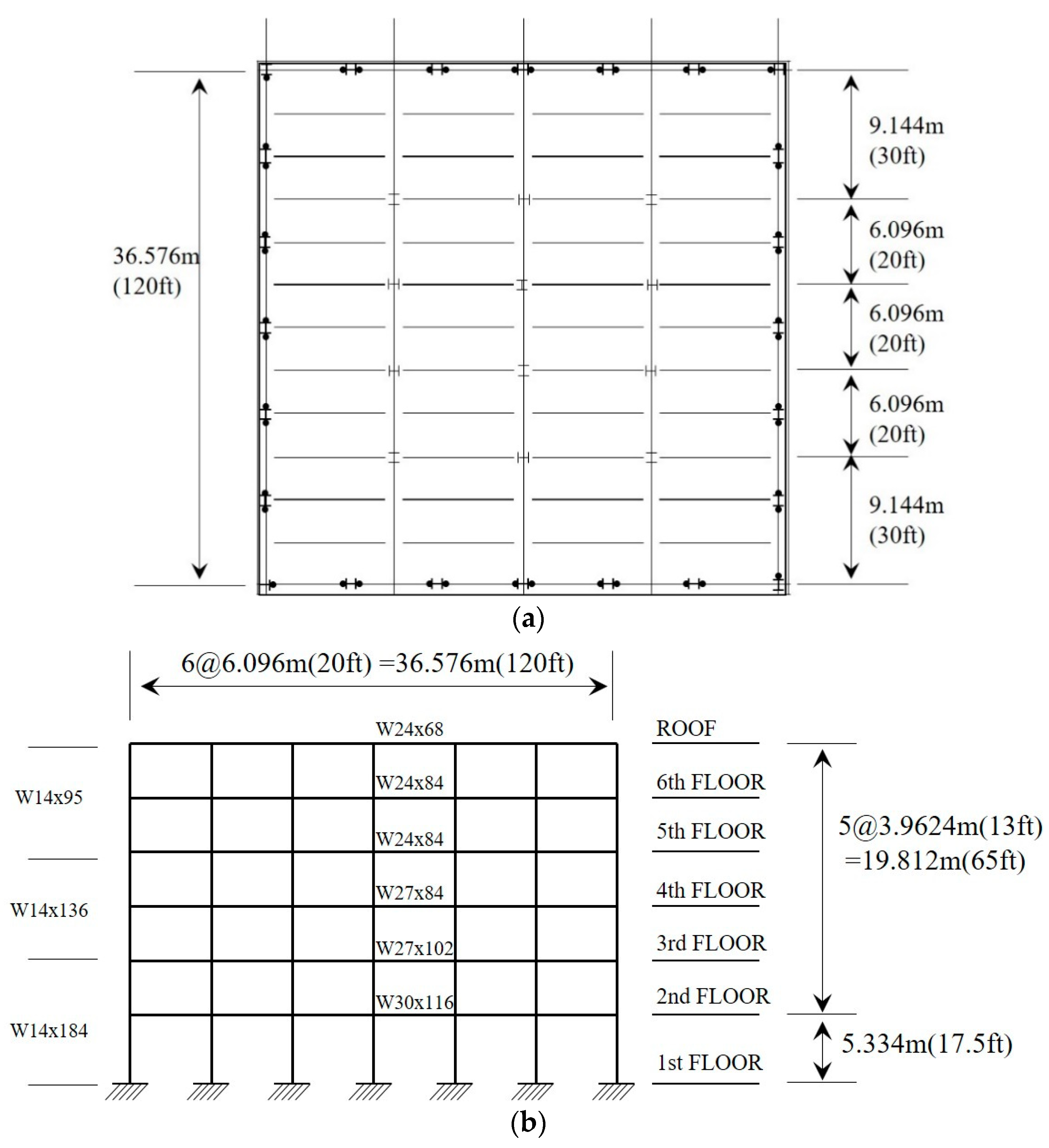
Figure 2 presents the plan view, member types, and the size of the structure. Numerical modeling of the target building was conducted using OpenSees that is extensively used for seismic analyses of structures. A two-dimensional (2D) numerical model was developed given that the target structure is symmetric, and force-based nonlinear beam-column elements and fiber sections were used to construct the 2D numerical model. Detailed descriptions of the numerical model of the target building are shown in Kunnath et al. [9] and Kalkan and Kunnath [36]. Kunnath et al. [9] established both the 2D and 3D models for the target building. They inferred that the response obtained from the 2D model was almost identical to the 3D model. This suggests that the use of a 2D model with one-half of the mass assigned to this frame is an adequate representation of the 3D building model used for symmetric building plans. Therefore, a 2D numerical model is adopted in this study.
Based on the structural configuration, we conducted the nonlinear analysis for the structure based on considerations of the seismic waves. The measured seismic waves were selected for magnitudes > 6.5, and a total of 135 historical data were obtained based on the considerations of far- and near-faults at the Pacific Earthquake Engineering Research Center (PEER). The 135 seismic waves were scaled and normalized based on the Peak Ground Acceleration (PGA) (that is the amplitude of the largest absolute acceleration). Nonlinear analysis using the normalized PGA was performed for each of the seismic intensity levels (between 0.0 g and 5.0 g for 125 points). Table 1 presents the ground motion database simulated for this study.
Typical machine learning algorithms compute different features. In this work, we used PGA, Peak Ground Velocity (PGV), Peak Ground Displacement (PGD), total Arias intensity, Cumulative Absolute Velocity (CAV), characteristic intensity, cumulative energy, significant duration (5% and 95%), Fourier amplitude spectrum, mean frequency, and mean period to investigate the structural response and a relationship according to the numerical analysis of seismic waves. In addition, the ratio of PGV and PGA, denoted as the PVA ratio, and the difference between the maximum seismic wave and the minimum seismic wave were considered in the model process [39]. Detailed information on the calculation of the seismic wave features used in the present analysis can be found in the paper of Papazafeiropoulos and Plevris [39].

2.2. Estimation Models

2.2.1. Linear Regression Model

In this study, we analyzed the model performance for the estimation of the maximum displacement of the structure and the seismic fragility curves. The linear regression model refers to the analysis conducted to obtain a linear relationship between the dependent variable, y, and the independent variable, x. The linear regression equation is based on the following assumptions.
(1)
Linearity: the linear relationship between x and y;
(2)
Independence: the lack of correlation between observations;
(3)
Homoscedasticity: the equality for the variance of residuals across the regression line;
(4)
Normality: the normal distribution for any fixed value of x and y.
In the analysis, the input seismic wave was used as an independent variable, and the parameter estimation of the model was used to predict the maximum displacement of the structure.

2.2.2. SVM Model

The SVM proposed by Vapnik [40] is a technique that solves the problem of the nonlinear regression by reconstructing data in high-dimensional space as a linear regression function. Based on the property, SVM can be used in various fields for classification and regression with the maximal margin hyperplane [41,42,43]. In SVM, the decision boundary was constructed by identifying the hyperplane that maximizes the margin, i.e., the distance between any two groups. The distance between the two groups is determined by the distance between the support vector and the support vector that represents the distance closest to the other group.
The SVM regression problem aims to identify a function to ensure that a weighted vector value (w) is within the actual target value (yi) and the maximum deviation ( δ ) for a given input vector value (xi) when m training data are provided to { ( x i , y i ) , , ( x m , y m ) | x i R n } with a pair of vectors of xi and yi [41]. The related equation is as follows:
f ( x )   =   w T x i + b
where T indicates the transpose of the matrix, and b implies the basis. When the function is determined, a slack variable is used to solve the block optimization problem. The function used to identify a solution for the optimization problem is as follows:
m i n 1 2 | | w | | 2 + C i   =   1 m ( ξ i + ξ i * )
s u b j e c t   t o   { y i w T x i b δ + ξ i w T x i + b y i δ + ξ i * ξ i , ξ i * 0
where C is a parameter that determines the complexity of the model as a penalty for an estimated error. If C is large, a larger penalty is allocated for the error with a low-generalization level. Conversely, if C is small, a smaller penalty is allocated for the error with a high-generalization level. Thus, selecting the appropriate value for C can adjust the complexity of the model and increase the generalized performance of the SVM regression. The slack variables that indicate the upper and lower conditions are denoted by ξ i and ξ i * , the following functions are used for SVM based on δ by ignoring errors within a certain distance.
ξ =   { 0                               i f   | ξ | δ | ξ | δ         o t h e r w i s e
In the SVM technique, the optimization problem of Equation (2), including the condition expressed by Equation (4), is solved using the Lagrange multiplier method, and the optimal solution is obtained by applying the Kernel function to the structure in the form of a nonlinear model. The detailed SVM model description and construction can be found in Vapnik [40].

2.2.3. Gaussian Process Regression Model

Gaussian process regression (GPR) analysis is a type of regression analysis technique that is conducted when the dependent variable follows a Gaussian process, and it has structural characteristics similar to those of the machine learning techniques. Assuming that the maximum displacement of a structure from an earthquake is a random variable, the expected displacement can be expressed as a function of the mean and covariance. The covariance can be interpreted as a kernel function. The GPR method can utilize a variety of models, such as the linear and nonlinear models, depending on the trend of the data to be applied to the analysis. If we determine the observed displacement as Xo, the predicted value as Xp, and the expected values of each variable as μ o and μ p , respectively, the covariance C can be expressed as ( X μ ) T ( X μ ) . If each data point is defined as Y o =   X o μ o and Y p   =   X p μ p following the Gaussian distribution, the simultaneous probability distribution is as follows:
p ( Y o , Y p ) e x p ( 1 2 [ Y o Y p ] T C 1 [ Y o Y p ] )
According to Bayes’ theorem, the following equation can be written as
p ( Y o , Y p ) e x p ( 1 2 ( Y o Y p C p p 1 C p o ) T ( C o o C o p C p p 1 C p o ) 1 ( Y o C o p C p p 1 Y p ) )
Equation (6) has the form of a normal distribution function and can be obtained through the multivariate Gaussian theorem [44]. The equation can also be listed as follows:
p ( Y o | Y p ) =   N ( μ o C o p C p p 1 ( X p μ p ) , C o o C o p C p p 1 C p o )
The values of μ o C o p C p p 1 ( X p μ p ) and C o o C o p C p p 1 C p o can be obtained based on the calculation using the kernel function. The defined GPR technique is distinguished from linear regression analysis in that it can use functions based on an infinite-dimensional characteristic, and can deal with uncertainties according to predictions. These properties are applicable for the estimation of variables of interest and trend analyses.

2.3. PCA

The PCA algorithm has been extensively used as a technique to reduce high-dimensional to low-dimensional vectors by obtaining the eigenvector of the covariance matrix that best expresses the characteristics of the data [45]. In other words, PCA reduces and summarizes multidimensional variables and derives new artificial variables by analyzing complex structures between correlated variables. The order of importance can be considered based on the size of the variation held by each principal component, and the first few components are transformed to hold as much of the total variation inherent in the original data as possible to minimize loss of information. This algorithm has been used in various fields in obtaining variables related to disasters [32].
Instead of using all available data when estimating the maximum displacement of a target structure, the model performance was improved with the use of selected key data while concurrently minimizing the loss of information in the dataset. In the analysis, if the ratio of the accumulated variance is set to 95%, the axis of the principal component with a 95% variance ratio is used as a model variable.

2.4. Evaluation Criteria

Cross-validation resampling techniques have been used to evaluate the performance of a model [33,34,35,46]. In this study, k-fold cross-validation was analyzed to validate the maximum displacement estimation and the performance of the proposed model. The k-fold cross-validation process allows the calculation of predicted errors, and estimates the boundaries for errors [31]. As the process can maintain more data in the training set, it is generally possible to lower the generalization error and achieve a better performance. If 5-fold is used, 20% of the data is excluded at each training step. Additionally, if 10-fold is used, 10% of the data is excluded. The model is then structured using the remaining data.
The performance of each model was evaluated using 5-fold cross-validation in the present study for the estimation of the maximum displacement of the structure. In the 5-fold cross-validation, the data were divided into five groups with similar sizes, and one of the groups was excluded from the data. The remaining data were trained, and the excluded groups were tested. To test the five groups, one of them was repeatedly excluded by considering the variability of the error. The measured results were compared and evaluated with statistical indicators, and the maximum displacement estimates were obtained for seismic fragility analysis.
For the evaluation of the proposed model, we estimated the statistical indices, including the R-squared (R2) and root-mean-squared error (RMSE). The indices were calculated using the following equations:
R 2 =   1 R S S T S S
RMSE =   1 n i =   1 n ( q i q ^ i ) 2
where TSS indicates the total sum of squares, and RSS denotes the residual sum of squares. Additionally, n denotes the total number of data, q i indicates the at-site estimate for location i, and q ^ i denotes the estimate derived from the models for location i. Figure 3 shows a simple diagram for the processes used to estimate the maximum displacement and fragility curves.

2.5. Seismic Probabilistic Risk Assessment

The seismic fragility curve developed for the seismic safety analysis was applied to the structural safety examination. This was achieved by the evaluation of the seismic performance of the structure and by the provision of a response standard to reduce damages from the earthquake [47]. In the study, the fragility curve was generated using the log-normal distribution function for seismic sensitivity analysis. Based on the performance of the seismic analysis, the probability of damage of the corresponding seismic intensity was obtained, and the function of seismic intensity was expressed as a log-normal distribution function within the seismic intensity range. The median value and log-standard deviation of the log-normal distribution function were obtained using maximum likelihood estimation. The maximum likelihood function applied to the study is,
L =   i =   1 N [ F ( a i ) ] x i [ 1 F ( a i ) ] 1 x i
where F ( · ) represents the fragility curve for the damaged object, and a i denotes the peak ground acceleration (PGA). In addition, x i has a value of x i   =   1 if the seismic damage occurs at the ith site. Otherwise, x i has a value of x i   =   0 . In this case, N is the total number of the observation sites. Subject to the log-normal assumption, F ( · ) can be represented by the following function:
F ( a )   =   Φ [ l n ( a c ) ζ ]
where a indicates the PGA, c is the median of the fragility curve for the damage condition, ζ denotes the standard deviation, and Φ [ · ] is the standardized normal distribution function.

3. Results

3.1. Estimation of Maximum Displacement

3.1.1. Comparison with Proposed Models

In the present study, we compared the performance of the models, including LR, SVM, and GPR, in the estimation of the maximum displacement of the structure based on PGA. The 5-fold cross-validation procedure was used for the evaluation of the three models. The model performance was also assessed based on the consideration of the normalization (NM) using a mean transformation and standardization (SD) for the data. The variables related to ground motion used for the model simulation were transformed to achieve normality and were standardized to gain consistent format. The transformed variables were then applied to the three models for the estimation of the maximum displacement by comparing the model results based on the nontransformed data.
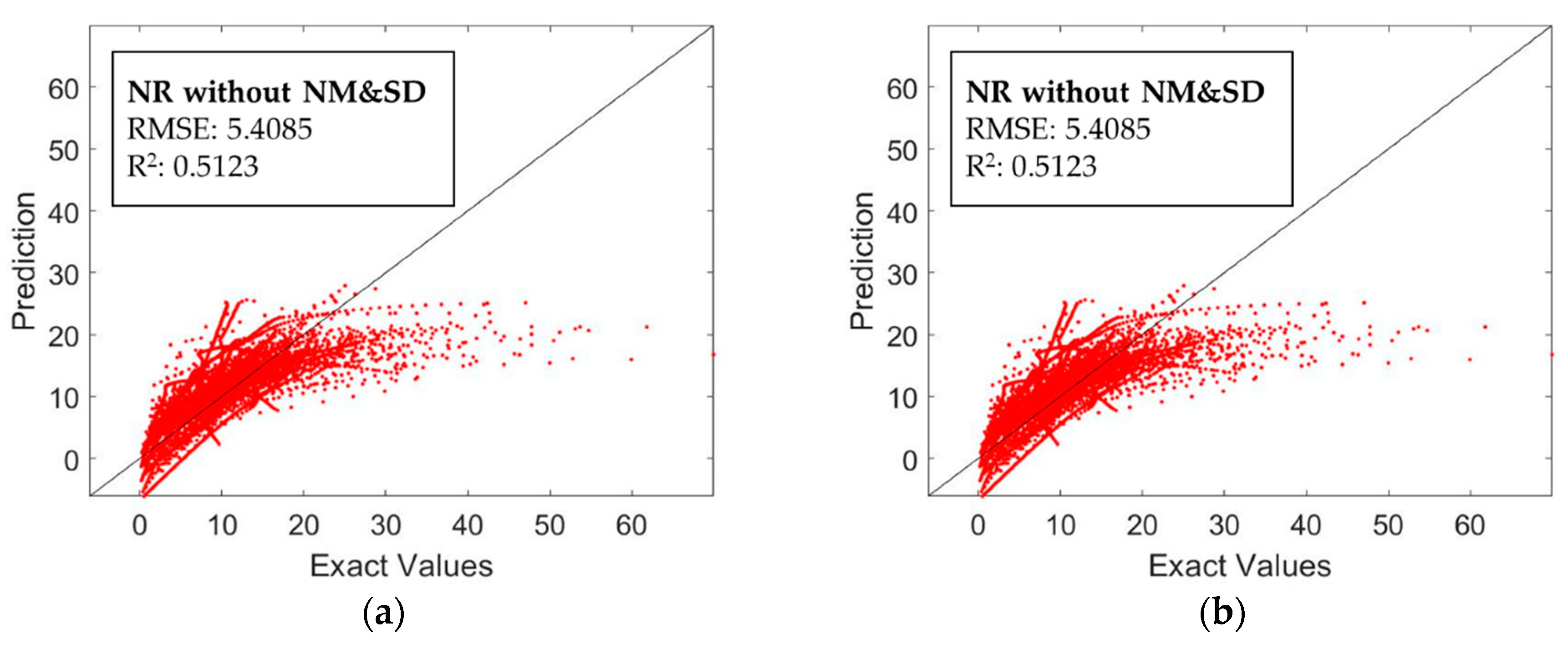
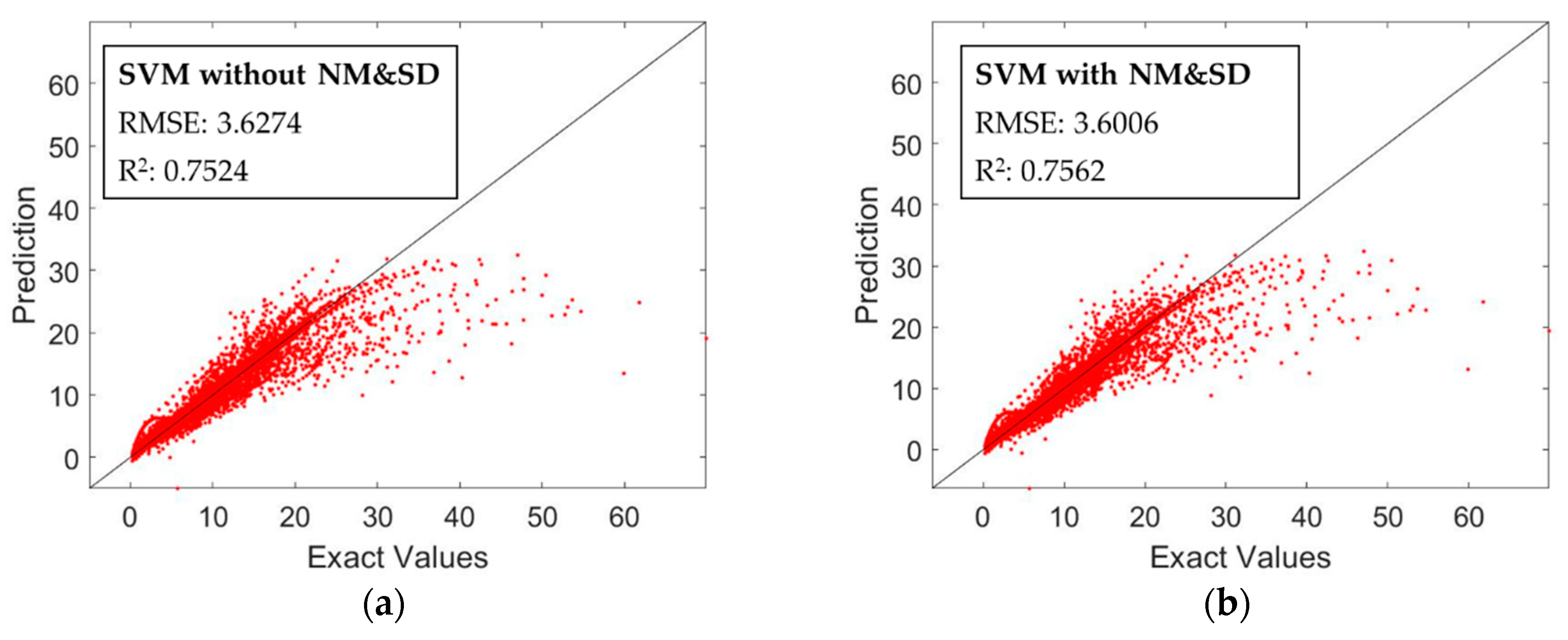
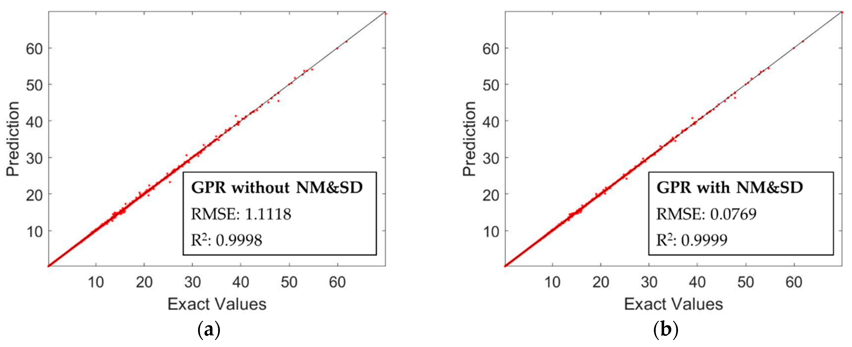
For the analysis of the estimated model, we investigated a relationship between the estimated and observed maximum displacements based on the three models. Figure 4 shows the relationship between the estimated and the observed displacements based on the LR model. Figure 4a presents the results without consideration of NM and SD, while Figure 4b shows the results based on the consideration of NM and SD. To estimate the displacement, all the collected variables were used for model simulations. The RMSE and R2 of LR are 5.4085 and 0.5123 for the model without and with NM and SD, respectively. There are no differences between the two models. Conversely, the RMSE and R2 for SVM and GPR seem to show model performance improvements when the NM and SD are considered in the process. The RMSE and R2 of SVM are 3.6274 and 0.7524 for the model without NM and SD, and 3.6006 and 0.7562 for the model with NM and SD, respectively. The RMSE and R2 of GPR are 0.1118 and 0.9998 for the model without NM and SD, and 0.0769 and 0.9999 for the model with NM and SD, respectively. Among the NR, SVM, and GPR, the GPR model provides the best performance based on the two statistical indices. Figure 5 and Figure 6 show the relationship between the estimated displacement and the observed displacement based on SVM and GPR.
Table 2 shows the results of the R2 and RMSE based on the models LR, SVM, and GPR with PGA. In the table, the GPR model clearly yields the best performance in the estimation of the maximum displacement of the structure. Moreover, when the NM and SD are used in the model procedure, the performance is improved by reducing the error of the estimation. The entries in bold font indicate the best results in the analyzed models in the study for PGA and SA. With the GPR model, we also investigated the use of PCA to enhance the performance of the model in the next section.

3.1.2. Consideration of PCA

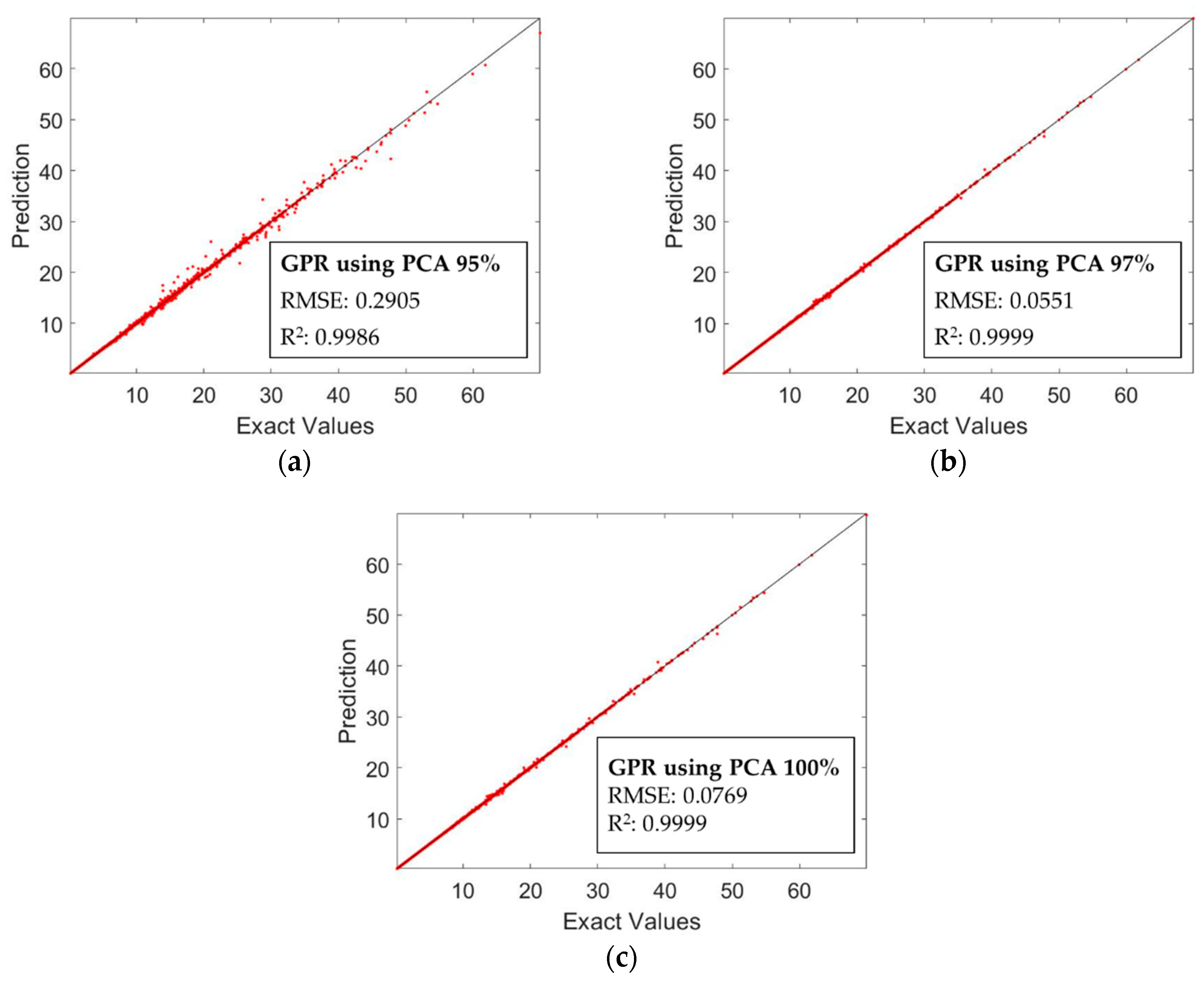
The GPR model was examined to obtain a better estimate of the maximum displacement by using PCA that reduces high-dimensional vectors with accurate results. PCA is an exploratory multivariate statistical approach used to simplify complex data sets. PCA was used to analyze seismic characteristics using datasets based on horizontal-to-vertical spectral ratio (HVSR or H/V) curves and establish the importance of HVSR patterns [48]. By examining various percentages of PCA with the GPR model, we aimed to provide the proper number of variables based on the seismic features to properly estimate the maximum displacement. In this study, the percentages of 95%, 97%, and 100% for PCA were considered by identifying the variance ratio. The PCA percentages of 95%, 97%, and 100% imply the use of seven, eight, and 13 variables in the model process, respectively. Figure 7 presents the relationship between the predicted maximum displacement and the observed maximum displacement with the use of the GPR with NM and SD. This figure shows the results based on the different percentages of PCA. In the figure, most of the results in the relationship represent a linear trend that indicates that the model performance is accurate. Thus, the GPR prediction result for the maximum displacement estimation reveals a satisfactory prediction quality to provide a rapid response from seismic activity.
Table 3 shows the results of the statistical indices including the R2 and RMSE values derived from the GPR model with various PCA percentages. In the table, the PCA value of 97% yields the best performance with an R2 value of 0.0551 and a RMSE value of 0.9999 for PGA. To produce the fragility curve based on the maximum displacement in the analysis, we used the model results with PCA values of 97% and 100%. This is because the results tend to yield a satisfactory performance in seismic analysis compared with the model with a PCA value of 95%. The eight variables used in the present study were based on the analysis of various percentages of PCA and seem to provide a good estimation.

3.2. Application of Fragility Analysis

After the prediction of the maximum displacement of the structure, a fragility curve was constructed to provide information about the risk of the structure owing to the earthquakes. In this study, a maximum inter-story drift ratio (MIDR) was selected as a performance criterion, and the development of the fragility curve was conducted using the two data, i.e., the exact data based on the simulation results, and the prediction data based on the GPR model with respect to the various seismic waves. The acceptance range of MIDR was classified as the levels of Immediate Occupancy (IO), Life Safety (LS), and Collapse Prevention (CP), based on the maximum height of the structure. These are three performance levels, and the threshold values were considered as the MIDR limits for the IO (0.7%), LS (2.5%), and CP (5.0%) levels, respectively [49,50].
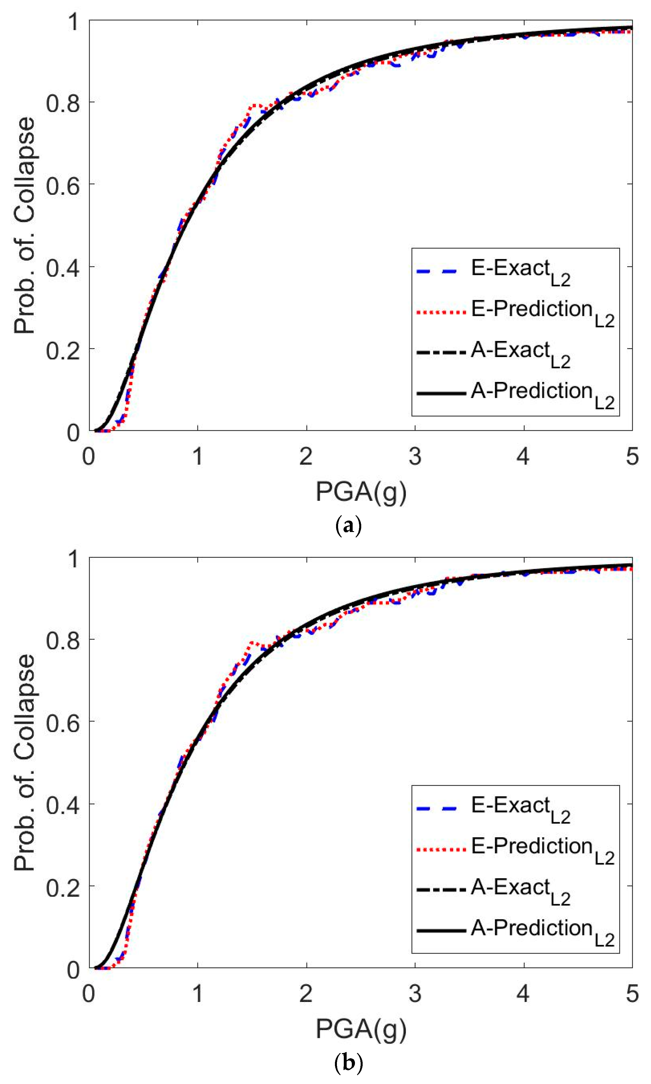
In Figure 8a, the results of the empirical and analytical fragility curves were presented based on the results of the actual analysis and the prediction for the LS level. The predicted results were obtained using the GPR model with a PCA of 97%. Figure 8b also shows the results of the empirical and analytical fragility curves based on the model with a PCA of 100%. From the figures, we inferred that the estimated fragility curves were similar to the empirical fragility curves and selected a PCA of 97% for the risk analysis based on the three parameters.
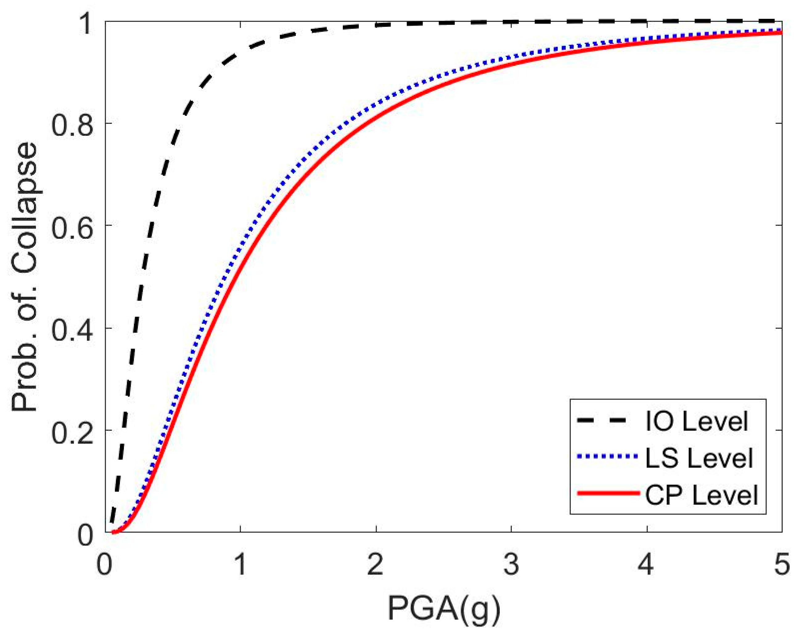
Figure 9 shows the model performance based on the fragility curves according to the GPR model with a PCA of 97%. This figure indicates the curves based on the IO, LS, and CP levels. From the figures, we can determine that the predicted curves match closely the empirical curves.
Table 4 shows the parameters of the fragility curves for each performance level derived from the numerical analysis and the estimated model based on a PCA of 97%. In the table, the estimated model yields accurate results compared with the numerical analysis outcomes. The results of the study indicate that the GPR model seems to possess an excellent potential for use and for the provision of the information of the seismic risk of the target structure with prompt response following a natural disaster.

4. Discussion

To identify the model performance with seismic risk analysis, we examined the PGA values by using various risk percentages. Table 5 lists the PGA values calculated for different seismic risks for the structure set at 16%, 50%, and 80%. These calculations were conducted with the use of the fragility curve derived from the model with a PCA of 97%. This table indicates that the results from the predicted data at 16%, 50%, and 80% based on the respective IO, LS, and CP levels yield similar values as the results from the exact data. From the table, we can also conclude that the proposed model provides relatively accurate estimates compared with the results of the model with the observed data at each performance level.

5. Conclusions

The present study aimed to analyze a prediction model used to estimate the maximum displacement of the structure with PGA. The estimated maximum displacement can be used to produce a fragility curve that is in turn used to achieve a rapid response from the seismic activity. The proposed model was designed using LR, SVM, and GPR, with datasets obtained from the numerical analyses of the seismic waves. The model performance was validated based on the RMSE, R2, and the various percentages of PCA. The fragility curves generated based on the empirical and the analytical methods were compared to identify the accuracy of the model.
In the analysis of the maximum displacement estimation, the LR, SVM, and GPR models were applied for the estimation of the displacement of the structure. Among the three models, the GPR model with NM and SD provided the best estimates with regard to the RMSE and R2 results. The R2 and RMSE derived from the model were 0.0769 and 0.9999, respectively, and the relationship between the estimated displacement and the observed displacement clearly exhibited a linear relationship. This result indicates that the GPR model with NM and SD based on the PGA may be a good application in the seismic analysis for responses from natural disasters.
Furthermore, the GPR model was analyzed to improve the performance with PCA values of 95%, 97%, and 100%. The model with a PCA value of 97% yielded the best performance in the estimation of the maximum displacement based on the statistical indices. Given the estimated maximum displacement according to the GPR model, the MIDR value that is commonly used for risk analysis of a structure was also calculated, and was used to examine the seismic fragility curve. Three performance levels, namely, IO, LS, and CP in MIDR, were investigated to compare the fragility curve parameters obtained from the actual numerical and predicted models. The results implied that the predicted parameters had accuracies that could provide robust responses. Therefore, the prediction model proposed in the study can quickly and precisely provide the displacement estimation of the structure subjected to the seismic activity. Accordingly, the same model can be applied for the evaluation of the structural safety.
Future research should focus on the extension of the maximum displacement using other models, such as the convolutional or recurrent neural networks that are types of deep-learning networks. Future studies should also examine other aspects correlated with the displacement of the structure. The extension of the variables in the estimation of the displacement and the production of the fragility curve can enhance the model estimates and reduce predicted damages from risk analysis. Future work should also focus on different structural types based on the GPR or other new techniques in the accurate estimation of the maximum seismic displacement of various buildings.

Author Contributions

Conceptualization, S.P. and K.J.; methodology, S.P. and K.J.; investigation, K.J., D.P., and S.P.; funding acquisition, K.J.; writing—review and editing, K.J., S.P., and D.P. All authors have read and agreed to the published version of the manuscript.

Funding

This research was supported by Basic Science Research Program through the National Research Foundation of Korea (NRF), funded by the Ministry of Education (grant number 2019R1I1A1A01061109) and by the Ministry of Science, ICT & Future Planning (grant number 2019R1A2C1007447).

Conflicts of Interest

The authors declare no conflict of interest.

References

  1. 2004 Indian Ocean Earthquake and Tsunami. Available online: https://en.wikipedia.org/wiki/2004_Indian_Ocean_earthquake_and_tsunami (accessed on 16 September 2020).
  2. 2008 Sichuan Earthquake. Available online: https://en.wikipedia.org/wiki/2008_Sichuan_earthquake (accessed on 16 July 2020).
  3. 2011 Tōhoku Earthquake and Tsunami. Available online: https://en.wikipedia.org/wiki/2011_T%C5%8Dhoku_earthquake_and_tsunami (accessed on 9 September 2020).
  4. 2016 Ecuador Earthquake. Available online: https://en.wikipedia.org/wiki/2016_Ecuador_earthquake (accessed on 25 August 2020).
  5. 2019 Peru Earthquake. Available online: https://en.wikipedia.org/wiki/2019_Peru_earthquake#:~:text=An%20earthquake%20measuring%20Mw,earthquake%20in%202019%20by%20magnitude (accessed on 31 August 2020).
  6. EPRI. Methodology for Developing Seismic Fragilities; Technical Report; Electric Power Research Institute: Palo Alto, CA, USA, 1994. [Google Scholar]
  7. Wang, Z.; Pedroni, N.; Zentner, I.; Zio, E. Seismic fragility analysis with artificial neural networks: Application to nuclear power plant equipment. Eng. Struct. 2018, 162, 213–225. [Google Scholar] [CrossRef] [Green Version]
  8. Kirçil, M.S.; Polat, Z.; Naganuma, T. Fragility analysis of mid-rise R/C frame buildings. Eng. Struct. 2006, 28, 1335–1345. [Google Scholar] [CrossRef]
  9. Kunnath, S.K.; Nghiem, Q.; El-Tawil, S. Modeling and response prediction in performance-based seismic evaluation: Case studies of instrumented steel moment-frame buildings. Earthq. Spectra 2004, 20, 883–915. [Google Scholar] [CrossRef]
  10. Vamvatsikos, D. Seismic Performance, Capacity and Reliability of Structures as Seen through Incremental Dynamic Analysis. Ph.D. Thesis, Stanford University, Stanford, CA, USA, 2002. [Google Scholar]
  11. Araya-Letelier, G.; Parra, P.F.; Lopez-Garcia, D.; Garcia-Valdes, A.; Candia, G.; Lagos, R. Collapse risk assessment of a Chilean dual wall-frame reinforced concrete office building. Eng. Struct. 2019, 183, 770–779. [Google Scholar] [CrossRef]
  12. Shafei, B.; Zareian, F.; Lignos, D.G. A simplified method for collapse capacity assessment of moment-resisting frame and shear wall structural systems. Eng. Struct. 2011, 33, 1107–1116. [Google Scholar] [CrossRef]
  13. EPRI. Seismic Probabilistic Risk Assessment Implementation Guide; Technical Report; Electric Power Research Institute: Palo Alto, CA, USA, 2013. [Google Scholar]
  14. Shinozuka, M.; Feng, M.Q.; Lee, J.; Naganuma, T. Statistical analysis of fragility curves. J. Eng. Mech. 2000, 126, 1224–1231. [Google Scholar] [CrossRef] [Green Version]
  15. Shinozuka, M.; Feng, M.Q.; Kim, H.-K.; Kim, S.-H. Nonlinear static procedure for fragility curve development. J. Eng. Mech. 2000, 126, 1287–1295. [Google Scholar] [CrossRef] [Green Version]
  16. Porter, K.; Kennedy, R.; Bachman, R. Creating fragility functions for performance-based earthquake engineering. Earthq. Spectra 2007, 23, 471–489. [Google Scholar] [CrossRef]
  17. Haselton, C.B.; Baker, J.W.; Liel, A.B.; Deierlein, G.G. Accounting for ground-motion spectral shape characteristics in structural collapse assessment through an adjustment for epsilon. J. Struct. Eng. 2011, 137, 332–344. [Google Scholar] [CrossRef] [Green Version]
  18. Lignos, D.G.; Krawinkler, H.; Whittaker, A.S. Prediction and validation of sidesway collapse of two scale models of a 4-story steel moment frame. Earthq. Eng. Struct. Dyn. 2011, 40, 807–825. [Google Scholar] [CrossRef]
  19. Baker, J.W. Efficient analytical fragility function fitting using dynamic structural analysis. Earthq. Spectra 2015, 31, 579–599. [Google Scholar] [CrossRef]
  20. Bakalis, K.; Vamvatsikos, D. Seismic fragility functions via nonlinear response history analysis. J. Struct. Eng. 2018, 144, 4018181. [Google Scholar] [CrossRef]
  21. Unnikrishnan, V.U.; Prasad, A.M.; Rao, B.N. Development of fragility curves using highdimensional model representation. Earthq. Eng. Struct. Dyn. 2013, 42, 419–430. [Google Scholar] [CrossRef]
  22. Seo, J.; Dueas-Osorio, L.; Craig, J.I.; Goodno, B.J. Metamodel-based regional vulnerability estimate of irregular steel moment-frame structures subjected to earthquake events. Eng. Struct. 2012, 45, 585–597. [Google Scholar] [CrossRef]
  23. Saha, S.K.; Matsagar, V.; Chakraborty, S. Uncertainty quantification and seismic fragility of base-isolated liquid storage tanks using response surface models. Probab. Eng. Mech. 2016, 43, 20–35. [Google Scholar] [CrossRef]
  24. Lagaros, N.D.; Fragiadakis, M. Fragility assessment of steel frames using neural networks. Earthq. Spectra 2007, 23, 735–752. [Google Scholar] [CrossRef]
  25. Mangalathu, S.; Jeon, J.-S.; DesRoches, R. Critical uncertainty parameters influencing seismic performance of bridges using lasso regression. Earthq. Eng. Struct. Dyn. 2018, 47, 748–801. [Google Scholar] [CrossRef]
  26. Jia, G.; Taflanidis, A.A. Kriging metamodeling for approximation of high-dimensional wave and surge responses in real-time storm/hurricane risk assessment. Comput. Methods Appl. Mech. Eng. 2013, 261, 24–38. [Google Scholar] [CrossRef]
  27. Ferrario, E.; Pedroni, N.; Zio, E.; Lopez-Caballero, F. Application of metamodel-based techniques for the efficient seismic analysis of structural systems. In Proceedings of the European Safety and Reliability Conference ESREL 2015, Zurich, Switzerland, 7–10 August 2015; CRC Press: Boca Raton, FL, USA, 2015; pp. 1193–1200. [Google Scholar]
  28. Calabresea, A.; Lai, C.G. Fragility functions of blockwork wharves using artificial neural networks. Soil Dyn. Earthq. Eng. 2013, 52, 88–102. [Google Scholar] [CrossRef]
  29. Ghosh, J.; Padgett, J.E.; Dueas-Osorio, L. Surrogate modeling and failure surface visualization for efficient seismic vulnerability assessment of highway bridges. Probab. Eng. Mech. 2013, 34, 189–199. [Google Scholar] [CrossRef]
  30. Gehl, P.; D’Ayala, D. Development of bayesian networks for the multi-hazard fragility assessment of bridge systems. Struct. Saf. 2016, 60, 37–46. [Google Scholar] [CrossRef]
  31. Basilevsky, A. Statistical Factor Analysis and Related Methods: Theory and Applications; John Wiley & Sons Inc.: London, UK, 1994. [Google Scholar]
  32. Chokmani, K.; Ouarda, T.B.M.J. Physiographical space-based kriging for regional flood frequency estimation at ungauged sites. Water Resour. Res. 2004, 40, W12514. [Google Scholar]
  33. Ouarda, T.B.M.J.; Shu, C. Regional low-flow frequency analysis using single and ensemble artificial neural networks. Water Resour. Res. 2009, 45. [Google Scholar] [CrossRef]
  34. Miller, R.G. A trustworthy jackknife. Ann. Math. Stat. 1964, 35, 1594–1605. [Google Scholar] [CrossRef]
  35. Shao, J.; Tu, D. The Jackknife and Bootstrap; Springer Science & Business Media: Berlin, Germany, 2012. [Google Scholar]
  36. Kalkan, E.; Kunnath, S.K. Effects of fling step and forward directivity on seismic response of buildings. Earthq. Spectra 2006, 22, 367–390. [Google Scholar] [CrossRef]
  37. Anderson, J.C.; Bertero, V.V. Implications of the Landers and Big Bear Earthquakes on Earthquake Resistant Design of Structures; Earthquake Engineering Research Center, University of California: Berkeley, CA, USA, 1997. [Google Scholar]
  38. Information for Strong-Motion Station Burbank—6-Story Commercial Bldg CGS—CSMIP Station 24370. Available online: https://strongmotioncenter.org/cgi-bin/CESMD/stationhtml.pl?stationID=CE24370&network=CGS (accessed on 16 July 2020).
  39. Papazafeiropoulos, G.; Plevris, V. OpenSeismoMatlab: A new open-source software for strong ground motion data processing. Heliyon 2018, 4, e00784. [Google Scholar] [CrossRef] [Green Version]
  40. Vapnik, V. The Nature of Statistical Learning Theory; Springer: New York, NY, USA, 1995. [Google Scholar]
  41. Kavzoglu, T.; Colkesen, I. A kernel functions analysis for support vector machines for land cover classification. Int. J. Appl. Earth. Obs. Geoinf. 2009, 11, 352–359. [Google Scholar] [CrossRef]
  42. Melgani, F.; Bruzzone, L. Classification of hyperspectral remote sensing images with support vector machines. IEEE Trans. Geosci. Remote Sens. 2004, 42, 1778–1790. [Google Scholar] [CrossRef] [Green Version]
  43. Jung, K.; Shin, J.-Y.; Park, D. A new approach for river network classification based on the beta distribution of tributary junction angles. J. Hydrol. 2019, 572, 66–74. [Google Scholar] [CrossRef]
  44. Rasmussen, C.E.; Williams, C.K.I. Gaussian Processes for Machine Learning; The MIT Press: Cambridge, UK, 2006. [Google Scholar]
  45. Jolliffe, I.T. Principal Component Analysis; Springer: New York, NY, USA, 2003. [Google Scholar]
  46. Jung, K.; Bae, D.-H.; Um, M.-J.; Kim, S.; Jeon, S.; Park, D. Evaluation of nitrate load estimations using neural networks and canonical correlation analysis with k-fold cross-validation. Sustainability 2020, 12, 400. [Google Scholar] [CrossRef] [Green Version]
  47. Nakamura, T.; Naganuma, T.; Shizuma, T.; Shinozuka, M. A Study on Failure Probability of Highway Bridge by Earthquake Based on Statistical Method. In Proceedings of the 10th Japanese Earthquake Engineering Symposium, Minato City, Tokyo, 25–27 November 1998. [Google Scholar]
  48. Paolucci, E.; Lunedei, E.; Albarello, D. Application of the principal component analysis (PCA) to HVSR data aimed at the seismic characterization of earthquake prone areas. Geophys. J. Int. 2017, 211, 650–662. [Google Scholar] [CrossRef]
  49. ASCE/SEI 41-06. Seismic Rehabilitation of Existing Buildings; Ameriacan Society of Civil Engineers: Reston, VA, USA, 2007. [Google Scholar]
  50. Rezaei, S.; Akbari Hamed, A.; Basim, M.C. Seismic performance evaluation of steel structures equipped with dissipative columns. J. Build. Eng. 2020, 29, 101227. [Google Scholar] [CrossRef]
Figure 1. Overview of the six-story target structure [38].
Sustainability 12 07803 g001
Figure 2. Structural configuration of 6-story residential structure with (a) plan view and (b) typical perimeter frame [9].
Sustainability 12 07803 g002
Figure 3. Diagram for model processes in obtaining the maximum displacement and fragility curves.
Sustainability 12 07803 g003
Figure 4. Relationship between the predicted displacement and the observed displacement for (a) LR without NM and SD and (b) LR with NM and SD.
Sustainability 12 07803 g004
Figure 5. Relationship between the predicted displacement and the observed displacement for (a) SVM without NM and SD and (b) SVM with NM and SD.
Sustainability 12 07803 g005
Figure 6. Relationship between the predicted displacement and the observed displacement for (a) GPR without NM and SD and (b) GPR with NM and SD.
Sustainability 12 07803 g006
Figure 7. Relationship between the predicted displacement and the observed displacement using GPR with PCA for (a) 95%, (b) 97%, and (c) 100%.
Sustainability 12 07803 g007
Figure 8. Empirical and Analytical Fragility Curves (a) PCA 97% and (b) PCA 100%.
Sustainability 12 07803 g008
Figure 9. Fragility Curves for PGA Cases including IO Level, LS Level, and CP Level.
Sustainability 12 07803 g009
Table 1. Ground Motion (GM) Database.
Ground Motion’s TypeDistanceNo. of GMs
Far-Field 10~1000 km67
Near-FieldPulse0~10 km34
No-Pulse0~10 km34
Total 135
Table 2. RMSE and R2 using LR, SVM, and GPR models for consideration of NM and SD.
Without NM & SDWith NM & SD
RMSER2RMSER2
LR5.410.515.410.51
SVM3.630.753.600.76
GPR0.110.99980.080.9999
Table 3. RMSE and R2 using GPR model with different percentages of PCA.
PCA 95%PCA 97%PCA 100%
GPR ModelRMSE0.29050.05510.0769
R20.99860.99990.9999
Table 4. Fragility curve parameters for IO, LS, and CP levels.
LevelExact DataPrediction Data
MedianSTDMedianSTD
IO0.280.820.280.83
LS0.890.850.890.83
CP0.960.850.970.82
Table 5. PGA value for the 16%, 50%, and 84% seismic risk of the target structure.
LevelPGA values(g)
Exact DataPrediction Data
16%50%84%16%50%84%
IO0.12350.28010.63510.12270.27920.6349
LS0.38100.88752.06760.38850.88552.0183
CP0.41430.96332.23960.42610.96742.1963