An Efficient Grid-Based K-Prototypes Algorithm for Sustainable Decision-Making on Spatial Objects

Abstract

Data mining plays a critical role in sustainable decision-making. Although the k-prototypes algorithm is one of the best-known algorithms for clustering both numeric and categorical data, clustering a large number of spatial objects with mixed numeric and categorical attributes is still inefficient due to complexity. In this paper, we propose an efficient grid-based k-prototypes algorithm, GK-prototypes, which achieves high performance for clustering spatial objects. The first proposed algorithm utilizes both maximum and minimum distance between cluster centers and a cell, which can reduce unnecessary distance calculation. The second proposed algorithm as an extension of the first proposed algorithm, utilizes spatial dependence; spatial data tends to be similar to objects that are close. Each cell has a bitmap index which stores the categorical values of all objects within the same cell for each attribute. This bitmap index can improve performance if the categorical data is skewed. Experimental results show that the proposed algorithms can achieve better performance than the existing pruning techniques of the k-prototypes algorithm.

1. Introduction

Sustainability is a concept for balancing environmental, economic and social dimensions with decision-making [1]. Data mining in sustainability is a very important issue since sustainable decision-making contributes to the transition to a sustainable society [2]. Data mining has been applied to solve wildlife preservation and biodiversity, balancing socio-economic needs and the environment, and large-scale deployment and management of renewable energy sources [3]. In particular, there is growing interest in spatial data mining in making sustainable decisions in geographical environments and national land policies [4].

Spatial data mining has become more and more important as spatial data collection increases due to technological developments, such as geographic information systems (GIS) and global positioning system (GPS) [5,6]. The four main techniques used in spatial data mining are spatial clustering [7], spatial classification [8], the spatial association rule [9], and spatial characterization [10]. Spatial clustering is a technique used to classify data with similar geographic and locational characteristics into the same group. It is an important component used to discover hidden knowledge in a large amount of spatial data [11]. Spatial clustering is also used in hotspot detection, which detects areas where specific events occur [12]. Hotspot detection is used in various scientific fields, including crime analysis [13,14,15], fire analysis [16] and disease analysis [17,18,19,20].

Most spatial clustering studies have focused on finding efficient way to isolate groups used for numeric data such as location information of spatial objects. However, many real-world spatial objects have categorical data, not just numeric data. Therefore, if the categorical data impacts spatial clustering results, the error value may be increased when the final cluster results are evaluated.

We have presented an example of disease analysis clustering using only spatial data. Suppose we are collecting disease-related data for a region in terms of disease location (the latitude and longitude on the global positioning system) and type of disease. The diseases are divided into three categories (i.e., p, q and r). Figure 1 shows 10 instances of disease-related data. If the similar data are grouped into three groups by only disease location, three groups are formed as follows: c₁(p₁, p₂, p₃, q4), c₂(q₁, q₂, q₃), and c₃(r₁, r₂, r₃). The representative attribute of cluster c₁ is set to p, so we are only concerned with p. Therefore, when q occurs in the cluster c₁ area, it is difficult to cope with. This is because three clusters are constructed using only location information of disease occurrence (spatial data). If the result from this example was used to affect a policy decision, it could result in a decision maker failing to carry out the correct policy. This is because the decision maker cannot carry out the policy on avian influenza in the area (20, 50).

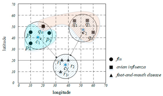
Figure 1. An example of clustering using location data.

Real world data is often a mixture of numeric data as well as categorical data. In order to apply the clustering technique to real world data, algorithms that consider categorical data are required. A representative clustering algorithm that uses mixed data is the k-prototypes algorithm [21]. The basic k-prototypes algorithm has large time complexity due to the processing of all of the data. Therefore, it is important to reduce the execution time in order to process the k-prototypes algorithm on large amounts of data. However, only a few studies have been conducted on how to reduce the time complexity of the k-prototypes algorithm. Kim [22] proposed a pruning technique to reduce distance computation between an object and cluster centers using the concept of partial distance computation. However, this method does not have high pruning efficiency due to the comparison of objects one by one with the cluster center.

In an effort to improve performance, we propose an effective grid-based k-prototypes algorithm, GK-prototypes, for clustering spatial objects. The proposed method makes use of the grid-based indexing technique, which improves pruning efficiency by comparing distance between cluster centers and a cell instead of distance between cluster centers and an object.

Spatial data can have geographic data as categorical attributes that indicate the characteristics of the object as well as the location of the object. Geographic data tends to have spatial dependence. Spatial dependence is the property of objects that are close to each other having increased similarities [23]. For example, soil types or network types are more likely to be similar at points one meter apart than at points one kilometer apart. Due to the nature of spatial dependence, the categorical data included in spatial data is often skewed because of the position of the object. In an effort to improve the performance of a grid-based k-prototypes algorithm, we take advantage of spatial dependence to the bitmap indexing technique.

The contributions of this paper are summarized as follows:

• We proposed an effective grid-based k-prototypes algorithm; GK-prototypes, which improves the performance of a basic k-prototypes algorithm.
• We developed a pruning technique which utilizes the minimum and maximum distance on numeric attributes and the maximum distance on categorical attributes between a cell and a cluster center.
• We developed a pruning technique based on a bitmap index to improve the efficiency of the pruning in case the categorical data is skewed.
• We provided several experimental results using real datasets and various synthetic datasets. The experimental results showed that our proposed algorithms achieve better performance than existing pruning techniques in the k-prototypes algorithm.

The organization of the rest of this paper is as follows. In Section 2, we overview spatial data mining, clustering for mixed data, the grid-based clustering algorithm and existing pruning technique in the k-prototypes algorithm. In Section 3, we first briefly describe notations and a basic k-prototypes algorithm. The proposed algorithm is explained in Section 4. In Section 5, experimental results on real and synthetic datasets demonstrate performance. Section 6 concludes the paper.

2. Related Works

2.1. Spatial Data Mining

Spatial data mining collectively refers to techniques that find useful knowledge from a set of spatial data. In general, spatial data mining has been broadly divided into the following areas: classification, association rule mining, co-location pattern mining, and clustering. Spatial classification is the task of labeling related groups according to specific criteria through spatial data attributes such as location information. As a method, research has been conducted on methods using decision trees [8], artificial neural networks [24,25], and multi-relational techniques [26]. Spatial association rule mining finds associations between spatial and non-spatial predicates. In [9], an efficient technique for mining strong spatial association rules was proposed. Mennis et al. demonstrates the application for the mining association rule from spatio-temporal databases [27]. Spatial co-location pattern mining discovers the subsets of Boolean spatial features that are frequently located together in geographic proximity [28]. Researches have been conducted to find spatial co-location patterns in spaces using Euclidean distance [29] and road network distance [30]. Spatial clustering is generally classified into partitioning based algorithms [31,32], density based algorithms [33,34], and grid-based algorithms (see Section 2.3). Among the partitioning based methods, the best known algorithm is a k-means [31] algorithm that classifies a dataset into k groups. Density-based spatial clustering of applications with noise (DBSCAN) [33] which is well known among the density based methods, determines the neighborhood of each datum and finds the groups considering the density of the data. Since all of the above algorithms are algorithms for numeric data, they are not directly applied to mixed data including categorical data.

2.2. Clustering for Mixed Data

Since real data is composed not only of numeric data but also of categorical data, clustering algorithms have been developed to handle mixed data (numeric and categorical data). The k-prototypes algorithm is the first proposed clustering algorithm to deal with mixed data types (numeric data and categorical data), which integrates k-means and k-modes algorithms [21]. Ahmad and Dey proposed a clustering algorithm based on k-means that handles mixed numeric and categorical data [35]. They proposed a distance measure and new cost function based on the co-occurrence of values in dataset, and provided a modified description of the cluster center to overcome the numeric data-only limitation of k-means algorithm. Hsu and Chen proposed a clustering algorithm based on variance and entropy (CAVE) which utilizes variance to measure the similarity of numeric data and entropy to calculate the similarity of categorical data [36]. Bohm et al. developed INTEGRATE to integrate the information provided by heterogeneous numeric and categorical attributes [37]. They used probability distributions based on information theory to model numeric and categorical attributes and minimized cost functions according to the principle of minimum description length. Ji et al. developed a modified k-prototypes algorithm which uses a new measure to calculate the dissimilarity between data objects and prototypes of clusters [38]. The algorithm utilizes the distribution centroid rather than the simple modes for representing the prototype of categorical attributes in a cluster. Ding et al. proposed an entropy-based density peaks clustering algorithm which provides a new similarity measure for either numeric or categorical attributes which has a uniform criterion [39]. Du et al. proposed a novel density peaks clustering algorithm for mixed data (DPC-MD) which uses a new similarity criterion to handle the three types of data: numeric, categorical, or mixed data for improving the original density peaks clustering algorithm [40]. Gu et al. proposed a modified k-prototypes algorithm to obtain the capacity of self-adaptive in discrete interval determination, which has overcome the shortcomings from common methods in conditional complementary entropy [41]. Davoodi et al. proposed a deep rule-based fuzzy system (DRBFS) which deals with a large amount of data with numeric and categorical attributes. The DRBFS provides an accurate in mortality prediction in the intensive care units in which the hidden layer is represented by interpretable fuzzy rules [42].

2.3. Grid-Based Clustering Algorithm

This subsection introduces grid-based algorithms mentioned in Section 2.2 in more detail. Grid-based techniques have the fastest processing time. They depend on the number of the grid cells instead of the number of objects in the data set [43]. The basic grid-based algorithm is as follows. A set of grid-cells is defined. In general, these grid-based clustering algorithms use a single uniform or multi-resolution grid cell to partition the entire dataset into cells. Each object is assigned to the appropriate grid cell and the density of each cell is computed. The cells which maintain a degree of density below a certain threshold are eliminated. In addition to the density of cells, the statistical information of objects within the cell is computed. After that, the clustering process is performed on the grid cells by using each cell’s statistical information instead of the objects itself.

The representative grid-based clustering algorithms are STING [44] and CLIQUE [45]. STING is a grid-based multi-resolution clustering algorithm in which the spatial area is divided into rectangular cells with a hierarchical structure. Each cell at a high level is divided into several smaller cells in the next lower level. For each cell in the pre-selected layer, the relevancy of the cell is checked by computing the confidence interval. If the cell is relevant, we include the cell in a cluster. If the cell is irrelevant, it is removed from further consideration. We look for more relevant cells at the next lower layer. This algorithm combines relevant cells into relevant regions and returns the clusters obtained. CLIQUE is a grid-based and density-based clustering algorithm used to identify subspaces of high dimensional data that allow better clustering quality than original data. CLIQUE partitions the n-dimensional data into non-overlapping rectangular units. The units are obtained by partitioning every dimension into certain intervals of equal length. The selectivity of a unit is defined as the total data points contained within it. A cluster in CLIQUE is a maximal set of connected dense units within a subspace. In a grid-based clustering study, the grid is used so that clustering is performed on the grid cells, instead of on the objects themselves. Chen et al. [46] proposes an algorithm called GK-means, which integrates grid structure and spatial index with a k-means algorithm. It focuses on choosing the better initial centers in order to improve the clustering quality and reduce the computational complexity of k-means.

Choi et al. proposed a k-partitioning algorithm for clustering large-scale spatio-textual dataset which uses a grid-based space partitioning scheme [47]. The fundamental idea of this algorithm is that an object in a cell is already spatially close to the other objects in the same cell, so it is sufficient to estimate their text cohesion. The grid-based approach has the disadvantage that the number of objects in each cell can be significantly different depending on how data points are distributed in space. To overcome this problem, this algorithm divides the entire set of objects into four subsets. The same partitioning process is performed repeatedly for each subset in such a way that all objects in each subset reside in one of the four quadrants. In this way, each cell will have a similar number of objects, even if they are not equal in length.

Most existing grid-based clustering algorithms regard objects in same cell of grid as a data point to process large scale data. Thus, the final clustering results of these algorithms are not the same as a basic k-prototype cluster result; all the cluster boundaries are either horizontal or vertical. In GK-means, the grid is used to select initial centers and remove noise data, but not used to reduce unnecessary distance calculation. To the best of our knowledge, a grid-based pruning technique that improves the performance of the k-prototypes algorithm has not been previously demonstrated.

2.4. Existing Pruning Technique in the K-Prototypes Algorithm

The k-prototypes algorithm spends most of the execution time computing the distance between an object and cluster centers. In order to improve the performance of the k-prototypes algorithm, Kim [22] proposed the concept of partial distance computation (PDC) which compares only partial attributes, not all attributes in measuring distance. The maximum distance that can be measured in one categorical attribute is 1. Thus, the distance that can be measured from the categorical attributes is bound to the number of categorical attributes, m-p. Given an object o and two cluster centers (c₁ and c₂), if the difference between d_r(o, c₁) and d_r(o, c₂) is more than m-p, we can know which clusters are closer to the object without the distance by using the categorical attributes. However, PDC is still not efficient because all objects are involved in the distance calculation and the characteristic (i.e., spatial dependence) of spatial data is not utilized in the clustering process.

3. Preliminary

In this section, we present some basic notations and definitions before describing our algorithms, and then discuss the basic k-prototypes algorithm. We summarize the notations used throughout this paper in Table 1.

Table 1. A summary of notations.

Notation	Description
O	a set of data
oi	i-th data in O
n	the number of objects
m	the number of attributes of an object
ci	the i cluster center point
gk	a cell of grid
d(oi, cj)	a distance between an object and an cluster center
dr(oi, cj)	a distance between an object and an cluster center for only numeric attributes
dc(oi, cj)	a distance between an object and an cluster center for only categorical attributes
dmin(gi, cj)	the minimum distance between a cell and a cluster center for only numeric attributes
dmax(gi, cj)	the maximum distance between a cell and a cluster center for only numeric attributes

The k-prototypes algorithm integrates the k-means and k-modes algorithms to allow for clustering data points described by mixed numeric and categorical attributes. Let a set of n objects be O = {o₁, o₂, …, o_n} where o_i = (o_i1, o_i2, …, o_im) is consisted of m attributes. The purpose of clustering is to partition n objects into k disjoint clusters C = {C₁, C₂, …, C_k} according to the degree of similarity of objects. The distance is used as a measure to group objects with high similarity into the same cluster. The distance d(o_i, C_j) between o_i and C_j is calculated as follows:

d(o_i, C_j) = d_r(o_i, C_j) + d_c(o_i, C_j)

(1)

where d_r(o_i, C_j) is the distance between numeric attributes and d_c(o_i, C_j) is the distance between categorical attributes.

$$d_r\left(o_i,C_j\right)={\displaystyle \sum }_{k=1}^p{\left|o_{ik}-c_{jk}\right|}^2$$

(2)

$$d_c\left(o_i,C_j\right)={\displaystyle \sum }_{k=p+1}^m\delta \left(o_{ik},c_{jk}\right)$$

(3)

$$\delta \left(o_{ik},c_{jk}\right)=\{\begin{array}{ccc}0,& when& o_{ik}=c_{jk}\\ 1,& when& o_{ik}\ne c_{jk}\end{array}$$

(4)

In Equation (2), d_r(o_i, C_j) is the squared Euclidean distance between an object and a cluster center on the numeric attributes. d_c(o_i, C_j) is the dissimilar distance on the categorical attributes, where o_ik and c_jk, 1 ≤ k ≤ p, are values of numeric attributes, o_ik and c_jk, p + 1 ≤ k ≤ m are values of categorical attributes. That is, p is the number of numeric attributes and m-p is the number of categorical attributes.

Consider a set of n objects, O = {o₁, o₂, …, o_n}. o_i = (o_i1, o_i2, …, o_im) is an object represented by m attribute values. The m attributes consist of m_r (the number of numeric attributes) and m_c (the number of categorical attributes), m = m_r + m_c. The distance between an object and a cluster center, d(o, c), is calculated by Equation (1). We adopt the data indexing technique based on the grid for pruning. The grid is decomposed into rectangular cells. We define the cells that make up the grid.

Definition 1.

A cell g in 2-dimension grid is defined by a start point vector S and an end point vector, cell g = (S, T), where S = [s₁, s₂] and T = [t₁, t₂].

Figure 2 depicts a fixed grid-based indexing a collection of 17 points and illustrates an example of definition of cells. Because objects have two numeric attributes, cells are defined in 2-dimension grid as follows: g₁ = ([0, 0], [10, 10]), and g₂ = ([20, 20], [30, 30]).

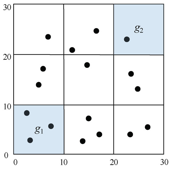
Figure 2. An example of definition of cell g.

Definition 2.

The minimum distance between a cell g_i and a cluster center c_j for numeric attributes, denoted d_min(g_i, c_j), is:

$$d_{\mathit{min}}(g_i,c_j)=\sqrt{{{\displaystyle \sum }}_{i=1}^{m_r}{\left|c_{ji}-r_i\right|}^2},$$

(5)

where $r_i=\{\begin{array}{l}\begin{array}{cc}{s}_i& if c_{ji}<s_i\end{array}\hfill \\ \begin{array}{cc}{t}_i& if c_{ji}>t_i\end{array}\hfill \\ \begin{array}{cc}{o}_i& otherwise\end{array}.\hfill \end{array}$

We use the classic Euclidian distance to measure the distance. If a cluster center is inside the cell, the distance between them is zero. If a cluster center is outside the cell, we use the Euclidean distance between the cluster center and the nearest edge of the cell.

Definition 3.

The maximum distance between a cell g_i and a cluster center c_j for numeric attributes, denoted d_max(g_i, c_j), is:

$$d_{\mathit{max}}(g_i,c_j)=\sqrt{{{\displaystyle \sum }}_{i=1}^{m_r}{\left|c_{ji}-r_i\right|}^2},$$

(6)

where $r_i=\{\begin{array}{l}\begin{array}{cc}{t}_i,& c_{ji}\le \frac{s_i+t_i}{2}\end{array}\hfill \\ \begin{array}{cc}{s}_i,& otherwise\end{array}\hfill \end{array}$

To distinguish between the two distances d_min and d_max, an example is illustrated in Figure 3, showing a cluster center (c₁), two cells (g₁ and g₂) and the corresponding distances.

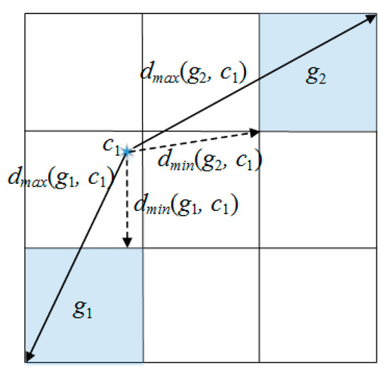
Figure 3. An example of distances d_min and d_max.

In a grid-based approach, d_min(g, c) and d_max(g, c) for a cell g and cluster centers c, are measured firstly before measuring the distance between an object and cluster centers. We can use d_min and d_max to improve performance of k-prototypes algorithm. Figure 3 shows an example of pruning using d_min and d_max. The object consists of 4 attributes (2 numeric and 2 categorical attributes).

In Figure 4, the maximum distance between g₁ and c₁, d_max(g₁, c₁) = 17($\sqrt{{\left(8-0\right)}^2+{\left(15-0\right)}^2}$). The minimum distance between g₁ and c₂, d_min(g₁, c₂) = 20 ($\sqrt{{\left(26-10\right)}^2+{\left(22-10\right)}^2}$). The d_max(g₁, c₁) is three less than d_min(g₁, c₂). Therefore, all objects in g₁ are closer to c₁ than c₂, if we are considering only numeric attributes. To find the closest cluster center from an object, we have to measure the distance by categorical attributes. If the difference between d_min and d_max is more than m_c (maximum distance by categorical attributes), however, the cluster closest to the object can be determined without using the distance, but instead by using categorical attributes. In Figure 4, the categorical data of c₁ is (a, z), and the categorical data of c₂ is (b, y). Assume that there are no objects in g₁ with ‘a’ in the first categorical attribute and ‘z’ in second categorical attribute. Since d_c(o, c₁) of all objects in g₁ is 2, maximum distance of all objects in g₁ is d_max(g₁, c₁) + 2. The maximum distance between c₁ and objects in g₁ is not less than the minimum distance between c₂ and objects in g₁. We can know that all objects in g₁ are closer to c₁ than c₂.

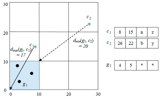
Figure 4. An example of the pruning method using minimum distance and maximum distance.

Lemma 1.

For any cluster centers c_i, c_j and any cell g_x, if d_min(g_x, c_j) − d_max(g_x, c_i) > m_c then, ∀o∈g_x, d(o, c_i) < d(o, c_j).

Proof. 

By assumption, d_min(g_x, c_j) > m_c + d_max(g_x, c_i). By Definition 2 and 3, d_min(g_x, c_i) ≤ d(c_i, o) ≤ d_max(g_x, c_i) + m_c, and d_min(g_x, c_j) ≤ d(c_j, o) ≤ d_max(g_x, c_j) + m_c. d(c_i, o) ≤ d_max(g_x, c_i) + m < d_min(g_x, c_j) ≤ d(c_j, o). ∀o∈g_x, d(c_i, o) < d(c_j, o).

Lemma 1 is the basis for our proposed pruning techniques. In the process of clustering, we first exploit Lemma 1 excluding cluster centers to be compared to objects.

4. GK-Prototypes Algorithm

In this section, we present two pruning techniques that are based on grids, for the purpose of improving the performance of the k-prototypes algorithm. The first pruning technique is KCP (K-prototypes algorithm with Cell Pruning) which utilizes d_min, d_max and the maximum distance on categorical attributes. The second pruning technique is KBP (K-prototypes algorithm with Bitmap Pruning) which utilizes bitmap indexes in order to reduce unnecessary distance calculation on categorical attributes.

4.1. Cell Pruning Technique

The computational cost of the k-prototypes algorithm is most often encountered when measuring distance between objects and cluster centers. To improve the performance, each object is indexed into a grid by numeric data in the data preparation step. We set up grid cells by storing two types of information. (a) The first is a start point vector S and an end point vector T, which is the range of the numeric value of the objects to be included in the cell (see Definition 1). Based on this cell information, the minimum and maximum distances between each cluster center and a cell are measured. (b) The second is bitmap indexes, which is explained in Section 4.2.

Algorithm 1 The k-prototypes algorithm with cell pruning (KCP)

Input: k: the number of cluster, G: the grid in which all objects are stored per cell

Output: k cluster centers

1: C[ ]← Ø // k cluster centers

2: Randomly choosing k object, and assigning it to C.

3: while IsConverged() do

4:  for each cell g in G

5:    dmin[ ], dmax[ ] ← Calc(g, C)

6:   dminmax ← min(dmax[ ])

7:   candidate ← Ø

8:   for j ←1 to k do

9:    if (dminmax + mc > dmin[j] ) // Lemma 1

10:     candidate ← candidate ∪ j

11:   end for

12:   min_distance ← ∞

13:   min_cluster ← null

14:   for each object o in g

15:    for each center c in candidate

16:     if min_distance > d(o, c)

17:      min_cluster ← index of c

18:   end for

19:   Assign(o, min_cluster)

20:   UpdateCenter(C[c])

21:  end for

22: end while

23: return C[k]

The details of cell pruning are as follows. First, we initialize an array C[j] to store the position of k cluster centers, 1 ≤ j ≤ k. Various initial cluster centers selection methods have been studied to improve the accuracy of clustering results in the k-prototypes algorithm [48]. Since we aim at improving the clustering speed, we adopt a simple method to select k objects randomly from input data and use them as initial cluster centers.

In general, the result of the clustering algorithm is evaluated after a single clustering process has been performed. Based on these evaluation results, it is determined whether the same clustering process must be repeated or terminated. The iteration is terminated if the sum of the difference between the current cluster center and the previous cluster center is less than a predetermined value (ε) as an input parameter by users. In Algorithm 1, we determine the termination condition through the IsConverged() function (line 3).

The Calc(g, C) function calculates the minimum and maximum distances between each cell g and k cluster centers (C) for each cluster center (line 4). The min and max distance tables for c₁ and c₂ are created as shown on the right side of Figure 5. The smallest distance among the maximum distance for g₁ is stored in the dminmax (line 5). In this example, 14.42 is stored in the dminmax. In the iteration step of clustering (line 6), the distance between objects and k cluster centers is measured by cells. The candidate stores the index number of the cluster center that needs to be measured from the cell. Through Lemma 1, if dminmax+m_c is greater than dmin[j], the j cluster center is included in the distance calculation, otherwise it is excluded (lines 8–11). For all cluster centers, only the cluster centers are to be measured and the distance from objects in the cell are finally left in the candidate. If the number of categorical attributes is 4, the sum of 4 and the maximum distance (14.42) between c₁ and g₁ is less than the minimum distance (19) between c₂ and g₁ in this example. Therefore, the objects in g₁ are considered to be closer to c₁ than c₂, without calculating the distance to c₂. Only c₁ is stored in the candidate, and c₂ is excluded. All objects in the cell are measured from the cluster centers in the candidate, d(o, c), (line 16). An object is assigned to the cluster where d(o, c) is computed as the smallest value using the Assign(o, min_cluster) function. The center of the cluster to which a new object is added is updated by remeasuring its cluster center using the UpdateCenter(C[c]) function. This clustering process is repeated until the end condition the IsConverged() returns a false.

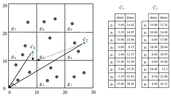
Figure 5. An example of minimum and maximum distance tables between 9 cells and 2 cluster centers.

4.2. Bitmap Pruning Technique

Spatial data tend to have similar categorical values in neighboring objects, and thus categorical data is often skewed. If we can utilize the characteristics of spatial data, the performance of the k-prototypes algorithm can be further improved. In this subsection, we introduce the KBP which can improve the efficiency of pruning when categorical data is skewed.

The KBP stores categorical data of all objects within a cell in a bitmap index. Figure 6 shows an example of storing categorical data as a bitmap index. Figure 6a is an example of spatial data. The x and y attributes indicate location information of objects as numeric data, and z and w attributes indicate features of objects as categorical data. For five objects in the same cell, g = {o₁, o₂, o₃, o₄, o₅}, Figure 6b shows the bitmap index structure where a row presents a categorical attribute and a column presents the categorical data of objects in same cell. A bitmap index consists of one vector of bits per attribute value, where the size of each bitmap is equal to the number of categorical data in the raw data. The bitmaps are encoded so that the i-th bit is set to 1 if the raw data has a value corresponding to the i-th column in the bitmap index, otherwise it is set to 0. For example, value 1 in z row and c column from the bitmap index means that value c exists in z attribute of the raw data. When the raw data is converted to a bitmap index, object id information is removed. We can quickly check for the existence of the specified value in the raw data using the bitmap index.

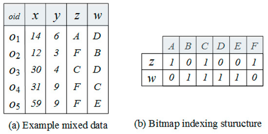
Figure 6. Bitmap indexing structure.

A maximum categorical distance is determined by the number of categorical attributes (m_c). If the difference of two numeric distances between one object and two cluster centers, |dr(o, c_i) − dr(o, c_j)|, is more than m_c, we can determine the cluster center closer to the object without categorical distance. However, since the numeric distance is not known in advance, we cannot determine the cluster center closer to the object using only categorical distance. Thus, the proposed KBP is utilized in reducing categorical distance calculations in the KCP. Algorithm 2 describes the proposed KBP. We explain only the extended parts from the KCP.

Algorithm 2 The k-prototypes algorithm with bitmap pruning (KBP)

Input: k: the number of cluster, G: the grid in which all objects are stored per cell

Output: k cluster centers

1: C[ ]← Ø // k cluster center

2: Randomly choosing k object, and assigning it to C.

3: while IsConverged() do

4:  for each cell g in G

5:    dmin[ ], dmax[ ] ← Calc(g, C)

6:   dminmax ← min(dmax[ ])

7:   arrayContain[] ← IsContain(g, C)

8:   candidate ← Ø

9:   for j ←1 to k do

10:    if (dminmax + mc > dmin[j] ) // Lemma 1

11:     candidate ← candidate ∪ j

12:    end for

13:   min_distance ← ∞

14:   min_cluster ← null

15:   distance ← null

16:   for each object o in g

17:    for each center c in candidate

18:     if (arrayContain [c] == 0)

19:      distance = dr(o, c) + mc

20:    else

21:      distance = dr(o, c) + dc(o, c)

22:    if min_distance > distance

23:     min_cluster ← index of cluster center

24:   end for

25:    Assign(o, min_cluster)

26:   UpdateCenter(C)

27:  end for

28: end while

29: return C[k]

To improve the efficiency of pruning categorical data, the KBP is implemented by adding two steps to the KCP. The first step is to find out whether the categorical attributes value of each cluster centers exists within the bitmap index of the cell by using the IsContain() function (line 7). The IsContain() function compares the categorical data of each cluster center with the bitmap index and returns 1 if there is more than one of the same data in the corresponding attribute. Otherwise, it returns 0. Demonstrated in Figure 6b, assume that we have a cluster center, c_i = (2, 5, D, A). The bitmap index does not have D in the z attribute and A in the w attribute. In this case, we know that there are no objects in the cell that have D in the z attribute and A in the w attribute. Therefore, the maximum categorical distance between all objects belonging to a cell and cluster center c_i is 0. Assume that we have another cluster center, c_j = (2, 5, A, B). The bitmap index has A in the z attribute and B in the w attribute. In this case, we know that there are some objects in the cell that have A in the z attribute or b in the w attribute. If one or more objects with the same categorical value are found in the corresponding attribute, the categorical distance calculation must be performed for all objects in the cell in order to determine the correct categorical distance. Finally, arrayContain[i] stores the result of the comparison between the i-th cluster center and the cell. In lines 8–12, the cluster centers that need to measure distance with each cell g are stored in the candidate, similar to the KCP. The second extended part (lines 18–23) is used to determine whether or not to measure the categorical distance using arrayContain. If arrayContain[i] has 0, the m_c is directly used as the result of the categorical distance without measuring the categorical distance (line 19).

4.3. Complexity

The complexity of the basic k-prototypes algorithm depends on the complexity of the classic Lloyd algorithm O(nkdi), where n is the number of objects, k the number of cluster centers, d the dimensionality of the data and i the number of iterations [49]. The complexity of the basic k-prototype algorithm is mainly dominated by the distance computation between objects and cluster centers. If our proposed algorithms cannot exclude objects from a distance computation in the worst case, the complexities of the proposed algorithms are also O(nkdi). However, our proposed algorithms based on heuristic techniques (KCP and KBP) can reduce the number of cluster centers to be computed, k’ ≤ k, and the number of dimensions to be computed, d’ ≤ d. Therefore, the time complexities of our proposed algorithms are O(nk’d’i), k’ ≤ k and d’ ≤ d.

For space complexity, KCP requires O(nd) to store the entire dataset, O(gm_r), where g is the number of cells, to store the start point vector S and the end point vector T of each cell, O(ktm_c), where t is the number of categorical data, to store the frequency of categorical data in each cluster and O(kd) to store cluster centers. KBP requires O(gtm_c) to store the bitmap index in each cell, where g is the number of cells. Therefore, the space complexities of KCP and KBP are O(nd + gm_r + ktm_c + kd) and O(nd + gm_r + ktm_c + kd + gtm_c), respectively.

5. Experiments

In this section, we evaluate the performance of the proposed GK-prototypes algorithms. For performance evaluation, we compare a basic k-prototypes algorithm (Basic), partial distance computation pruning (PDC) [22] and our two algorithms (KCP and KBP). We examined the performance of our algorithms as the number of objects, the number of clusters, the number of categorical attributes and the number of divisions in each dimension increased. In Table 2, the parameters used for the experiments are summarized. The righthand column of the table illustrates the baseline values of the various parameters. For each set of parameters, we perform 10 sets of experiments and the average values are reported. Even under the same parameter values, the number of clustering iterations will vary if the input data is different. Therefore, we measure the performance of each algorithm with the average execution time it takes for clustering to repeat once.

Table 2. Parameters for the experiments.

Parameter	Description	Baseline Value
n	no. of objects	1000 K
k	no. of clusters	10
mr	no. of numeric attributes	2
mc	no. of categorical attributes	5
s	no. of division in each dimensions	10

The experiments are carried out on a PC with Intel(R) Core(TM) i7 3.5 GHz, 32GB RAM. All the algorithms are implemented in Java.

5.1. Data Sets

The experiments use both real datasets and synthetic datasets. We generate various synthetic datasets with numeric attributes and categorical attributes. For numeric attributes in each dataset, two numeric attributes are generated in the 2D space [0, 100] × [0, 100] to indicate an object’s location. Each object is assigned into s × s cells within a grid using numeric data. The numeric data is generated according to uniform distributions in which numeric data is selected [0, 100] randomly or with Gaussian distributions with mean = 50 and standard deviation = 10. The categorical data is generated according to uniform distributions or skewed distributions. For uniform distributions, we select a letter from A to Z randomly. For skewed distributions, we generate categorical data in such a way that objects in same cell have similar letters based on their numeric data. For real datasets, we use the postcodes with easting, northing, latitude, and longitude which contains 1,048,576 British postcodes (from https://www.getthedata.com/open-postcode-geo).

5.2. Effects of the Number of Objects

To illustrate scalability, we vary the number of objects from 100 K to 1000 K. Other parameters are given baseline values (Table 2). Figure 7, Figure 8, Figure 9 and Figure 10 show the effect of the number of objects. Four graphs are shown in a linear scale. For each algorithm, the runtime per iteration is approximately proportional to the number of objects.

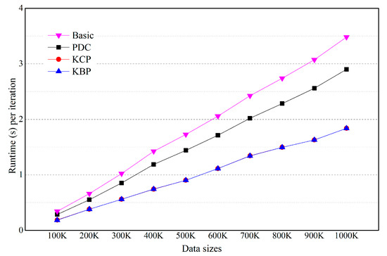
Figure 7. Effect of the number of objects (numeric data and categorical data are on uniform distribution).

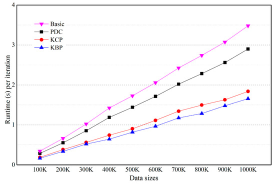
Figure 8. Effect of the number of objects (numeric data is on uniform distribution and categorical data is on skewed distribution).

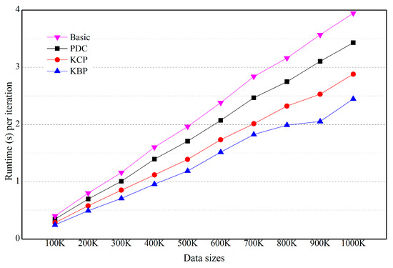
Figure 9. Effect of the number of objects (numeric data is on Gaussian distribution and categorical data is on skewed distribution).

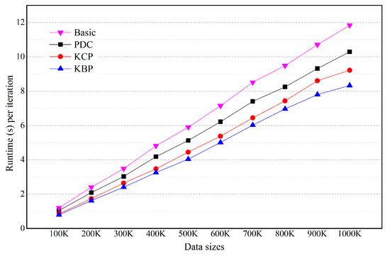
Figure 10. Effect of the number of objects on real datasets.

In Figure 7, KBP and KCP outperforms PDC and Basic. However, there is little difference in the performance between KBP and KCP. This is because if the categorical data has uniform distribution, most of the categorical data exists in the bitmap index. In this case, KBP is the same performance as KCP.

In Figure 8, KBP outperforms KCP, PDC and Basic. For example, KBP runs up to 1.1, 1.75 and 2.1 times faster than KCP, PDC and Basic, respectively (n = 1000 K). If categorical data is on a skewed distribution, KBP is effective at improving performance. As the size of the data increases, the difference in execution time increases. This is because as the data size increases, the amount of distance calculation increases, while at the same time the number of objects included in the cluster being pruned increases. In Figure 9, KCP outperforms PDC. Even if the numeric data is on a Gaussian distribution, cell pruning is effective at improving performance.

In Figure 10, KBP outperforms KCP, PDC and Basic on real datasets. For example, KBP runs up to 1.1, 1.23 and 1.42 times faster than KCP, PDC and Basic, respectively (n = 1000 K). KBP is effective at improving performance because the categorical data of the actual data is not uniform. As the size of the data increases, the difference in execution time increases. The reason is because as the data size increases, the amount of distance calculation increases, while at the same time the number of objects included in the cluster being pruned increases.

5.3. Effects of the Number of Clusters

To confirm the effects of the number of clusters, we vary the number of clusters, k, from 5 to 20. Other parameters are kept at their baseline values (Table 2). Figure 11, Figure 12, Figure 13 and Figure 14 show the effects of the number of clusters. Four graphs are also shown in a linear scale. For each algorithm, the runtime is approximately proportional to the number of clusters.

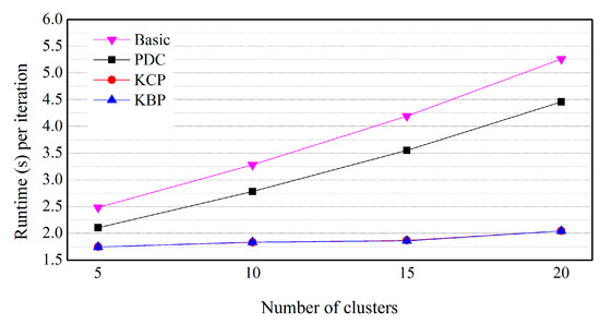
Figure 11. Effect of the number of clusters (numeric data and categorical data are on uniform distribution).

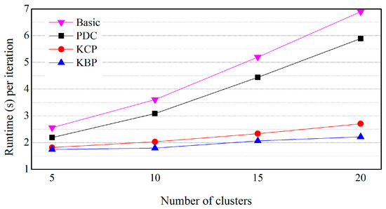
Figure 12. Effect of the number of clusters (numeric data are uniformly distributed and the distribution of categorical data is skewed).

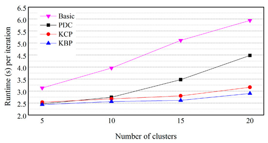
Figure 13. Effect of the number of clusters (numeric data is on Gaussian distribution and categorical data is on skewed distribution).

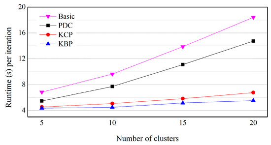
Figure 14. Effect of the number of clusters on real data.

In Figure 11, KBP and KCP also outperform PDC and Basic. However, there is also little difference in performance between KBP and KCP. This is because if the categorical data has uniform distribution, most of the categorical data exists in the bitmap index similar to Figure 7.

In Figure 12, KBP outperforms KCP, PDC and Basic. For example, KBP runs up to 1.13, 1.71 and 2.01 times faster than KCP, PDC and Basic, respectively (k = 10). This result indicates that KBP is effective for improving performance even if categorical data is on a skewed distribution. As the number of clusters increases, the difference in execution time increases. This is also because as the data size increases, the amount of distance calculation increases, while at the same time the number of objects included in the cluster being pruned increases in a similar way to Figure 8. In Figure 13, KCP also outperforms PDC and Basic. Even if the numeric data is on a Gaussian distribution, KCP is also effective at improving performance.

In Figure 14, KBP outperforms KCP, PDC and Basic on real datasets. For example, KBP runs up to 1.09, 1.68 and 2.14 times faster than KCP, PDC and Basic, respectively (k = 10). As the number of clusters increases, the difference in execution time increases. This is also because as the data size increases, the amount of distance calculation increases, while at the same time the number of objects included in the cluster being pruned increases in a similar way to Figure 8. In Figure 14, KCP also outperforms PDC and Basic. Even if the numeric data is on a Gaussian distribution, KCP is also effective at improving performance.

5.4. Effects of the Number of Categorical Attributes

To confirm the effects of the number of categorical attributes, we vary the number of categorical attributes from 5 to 20. Other parameters are given baseline values. Figure 15 shows the effect of the number of categorical attributes. The graph is also shown in a linear scale. For each algorithm, the runtime per iteration is approximately proportional to the number of categorical attributes. KBP outperforms KCP and PDC. For example, KBP runs up to 1.13 and 1.71 times faster than KCP and PDC, respectively (m_c = 5). Even if the number of categorical attributes increases, the difference between the execution time of KCP and PDC is kept almost constant. The reason is that KCP is based on numeric attributes and is not affected by the number of categorical attributes.

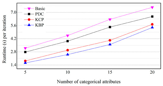
Figure 15. Effect of the number of categorical attributes on a skewed distribution.

5.5. Effects of the Size of Cells

To confirm the effects of the size of cells, we vary the number of cells from 5 to 20. Other parameters are given baseline values (Table 2). Figure 16 shows the effect of the number of divisions in each dimension. KBP and KCP outperform PDC. In Figure 16, the horizontal axis is the number of divisions of each dimension. As the number of divisions increases, the size of the cell decreases. As the cell size gets smaller, the distance between the cell and cluster centers can be measured more accurately. There is no significant difference in execution time according to the size of the cell by each algorithm. This is because the distance calculation between the cell and the cluster center is increased in proportion to the number of cells. The bitmap index stored by the cell is also increased.

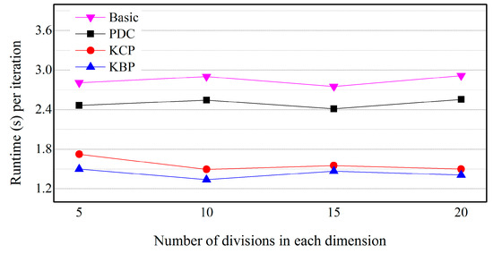
Figure 16. Effect of the number of cells on a skewed distribution.

6. Conclusions

In this paper we proposed an efficient grid-based k-prototypes algorithm, GK-prototypes, that improves performance for clustering spatial objects. We developed two pruning techniques, KCP and KBP. KCP, which uses both maximum and minimum distance between cluster centers and a cell, improves performance more than PDC and Basic. KBP is an extension of cell pruning to improve the efficiency of pruning in case a categorical data is skewed. Our experimental results demonstrate that KCP and KBP outperform PDC and Basic, and KBP outperforms KCP, except with uniform distributions of categorical data. These results lead us to the conclusion that our grid-based k-prototypes algorithm achieves better performance than the existing k-prototypes algorithm. The grid-based indexing technique for numeric attributes and a bitmap indexing technique for categorical attributes are effective at improving the performance of the k-prototypes algorithm.

As data has grown exponentially and more complex, traditional clustering algorithms face great challenges dealing with them. In future work, we may consider optimized pruning techniques of the k-prototypes algorithm in a parallel processing environment.

References

- Zavadskas, E.K.; Antucheviciene, J.; Vilutiene, T.; Adeli, H. Sustainable Decision Making in Civil Engineering, Construction and Building Technology. Sustainability 2018, 10, 14. [Google Scholar] [CrossRef]
- Hersh, M.A. Sustainable Decision Making: The Role of Decision Support systems. IEEE Trans. Syst. Man Cybern. C Appl. Rev. 1999, 29, 395–408. [Google Scholar] [CrossRef]
- Gomes, C.P. Computational Sustainability: Computational Methods for a Sustainable Environment, Economy, and Society. Bridge Natl. Acad. Eng. 2009, 39, 8. [Google Scholar]
- Morik, K.; Bhaduri, K.; Kargupta, H. Introduction to Data Mining for Sustainability. Data Min. Knowl. Discov. 2012, 24, 311–324. [Google Scholar] [CrossRef]
- Aissi, S.; Gouider, M.S.; Sboui, T.; Said, L.B. A Spatial Data Warehouse Recommendation Approach: Conceptual Framework and Experimental Evaluation. Hum.-Centric Comput. Inf. Sci. 2015, 5, 30. [Google Scholar] [CrossRef]
- Kim, J.-J. Spatio-temporal Sensor Data Processing Techniques. J. Inf. Process. Syst. 2017, 13, 1259–1276. [Google Scholar] [CrossRef]
- Sander, J.; Ester, M.; Kriegel, H.P.; Xu, X. Density-Based Clustering in Spatial Databases: The Algorithm GDBSCAN and Its Applications. Data Min. Knowl. Discov. 1998, 2, 169–194. [Google Scholar] [CrossRef]
- Koperski, K.; Han, J.; Stefanovic, N. An Efficient Two-Step Method for Classification of Spatial Data. In Proceedings of the International Symposium on Spatial Data Handling (SDH’98), Vancouver, BC, Canada, 12–15 July 1998; pp. 45–54. [Google Scholar]
- Koperski, K.; Han, J. Discovery of Spatial Association Rules in Geographic Information Databases. In Proceedings of the 4th International Symposium on Advances in Spatial Databases (SSD’95), Portland, ME, USA, 6–9 July 1995; pp. 47–66. [Google Scholar]
- Ester, M.; Frommelt, A.; Kriegel, H.P.; Sander, J. Algorithms for Characterization and Trend Detection in Spatial Databases. In Proceedings of the Fourth International Conference on Knowledge Discovery and Data Mining (KDD’98), 27–31 August 1995; pp. 44–50. [Google Scholar]
- Deren, L.; Shuliang, W.; Wenzhong, S.; Xinzhou, W. On Spatial Data Mining and Knowledge Discovery. Geomat. Inf. Sci. Wuhan Univ. 2001, 26, 491–499. [Google Scholar]
- Boldt, M.; Borg, A. A Statistical Method for Detecting Significant Temporal Hotspots using LISA Statistics. In Proceedings of the Intelligence and Security Informatics Conference (EISIC), Athens, Greece, 27–31 September 2017. [Google Scholar]
- Yu, Y.-T.; Lin, G.-H.; Jiang, I.H.-R.; Chiang, C. Machine-Learning-Based Hotspot Detection using Topological Classification and Critical Feature Extraction. In Proceedings of the 50th Annual Design Automation Conference, Austin, TX, USA, 29 May–7 June 2013; pp. 460–470. [Google Scholar]
- Murray, A.; McGuffog, I.; Western, J.; Mullins, P. Exploratory Spatial Data Analysis Techniques for Examining Urban Crime. Br. J. Criminol. 2001, 41, 309–329. [Google Scholar] [CrossRef]
- Chainey, S.; Tompson, L.; Uhlig, S. The Utility of Hotspot Mapping for Predicting Spatial Patterns of Crime. Secur. J. 2008, 21, 4–28. [Google Scholar] [CrossRef]
- Di Martino, F.; Sessa, S. The Extended Fuzzy C-means Algorithm for Hotspots in Spatio-temporal GIS. Expert. Syst. Appl. 2011, 38, 11829–11836. [Google Scholar] [CrossRef]
- Di Martino, F.; Sessa, S.; Barillari, U.E.S.; Barillari, M.R. Spatio-temporal Hotspots and Application on a Disease Analysis Case via GIS. Soft Comput. 2014, 18, 2377–2384. [Google Scholar] [CrossRef]
- Mullner, R.M.; Chung, K.; Croke, K.G.; Mensah, E.K. Geographic Information Systems in Public Health and Medicine. J. Med. Syst. 2004, 28, 215–221. [Google Scholar] [CrossRef] [PubMed]
- Polat, K. Application of Attribute Weighting Method Based on Clustering Centers to Discrimination of linearly Non-separable Medical Datasets. J. Med. Syst. 2012, 36, 2657–2673. [Google Scholar] [CrossRef] [PubMed]
- Wei, C.K.; Su, S.; Yang, M.C. Application of Data Mining on the Development of a Disease Distribution Map of Screened Community Residents of Taipei County in Taiwan. J. Med. Syst. 2012, 36, 2021–2027. [Google Scholar] [CrossRef] [PubMed]
- Huang, Z. Clustering Large Data Sets with Mixed Numeric and Categorical Values. In Proceedings of the First Pacific Asia Knowledge Discovery and Data Mining Conference, Singapore, 22–24 July 1997; pp. 21–34. [Google Scholar]
- Kim, B. A Fast K-prototypes Algorithm using Partial Distance Computation. Symmetry 2017, 9, 58. [Google Scholar] [CrossRef]
- Goodchild, M. Geographical Information Science. Int. J. Geogr. Inf. Sci. 1992, 6, 31–45. [Google Scholar] [CrossRef]
- Fischer, M.M. Computational Neural Networks: A New Paradigm for Spatial Nalysis. Environ. Plan. A 1998, 30, 1873–1891. [Google Scholar] [CrossRef]
- Yao, X.; Thill, J.-C. Neurofuzzy Modeling of Context–contingent Proximity Relations. Geogr. Anal. 2007, 39, 169–194. [Google Scholar] [CrossRef]
- Frank, R.; Ester, M.; Knobbe, A. A Multi-relational Approach to Spatial Classification. In Proceedings of the 15th ACM SIGKDD International Conference on Knowledge Discovery and Data Mining, 28 June–1 July 2009; pp. 309–318. [Google Scholar]
- Mennis, J.; Liu, J.W. Mining Association Rules in Spatio-temporal Data: An Analysis of Urban Socioeconomic and Land Cover Change. Trans. GIS 2005, 9, 5–17. [Google Scholar] [CrossRef]
- Shekhar, S.; Huang, Y. Discovering Spatial Co-location Patterns: A Summary of Results. In Advances in Spatial and Temporal Databases (SSTD 2001); Jensen, C.S., Schneider, M., Seeger, B., Tsotras, V.J., Eds.; Springer: Berlin/Heidelberg, Germany, 2001. [Google Scholar]
- Wan, Y.; Zhou, J. KNFCOM-T: A K-nearest Features-based Co-location Pattern Mining Algorithm for Large Spatial Data Sets by Using T-trees. Int. J. Bus. Intell. Data Min. 2009, 3, 375–389. [Google Scholar] [CrossRef]
- Yu, W. Spatial Co-location Pattern Mining for Location-based Services in Road Networks. Expert. Syst. Appl. 2016, 46, 324–335. [Google Scholar] [CrossRef]
- Hartigan, J.A.; Wong, M.A. Algorithm as 136: A K-means Clustering Algorithm. J. R. Stat. Soc. 1979, 28, 100–108. [Google Scholar] [CrossRef]
- Sharma(sachdeva), R.; Alam, A.M.; Rani, A. K-Means Clustering in Spatial Data Mining using Weka Interface. In Proceedings of the International Conference on Advances in Communication and Computing Technologies, Chennai, India, 3–5 August 2012; pp. 26–30. Available online: https://www.ijcaonline.org/proceedings/icacact/number1/7970-1006 (accessed on 12 July 2018).
- Ester, M.; Kriegel, H.P.; Sander, J.; Xu, X. Density-based Algorithm for Discovering Clusters in Large Spatial Databases with Noise. In Proceedings of the Second International Conference on Knowledge Discovery and Data Mining, Portland, OR, USA, 2–4 August 1996; AAAI Press: Portland, OR, USA, 1996; pp. 226–231. [Google Scholar]
- Kumar, K.M.; Reddy, A.R.M. A Fast DBSCAN Clustering Algorithm by Accelerating Neighbor Searching using Groups Method. Pattern Recognit. 2016, 58, 39–48. [Google Scholar] [CrossRef]
- Ahmad, A.; Dey, L. A K-mean Clustering Algorithm for Mixed Numeric and Categorical Data. Data Knowl. Eng. 2007, 63, 503–527. [Google Scholar] [CrossRef]
- Hsu, C.-C.; Chen, Y.-C. Mining of Mixed Data with Application to Catalog Marketing. Expert Syst. Appl. 2007, 32, 12–23. [Google Scholar] [CrossRef]
- Böhm, C.; Goebl, S.; Oswald, A.; Plant, C.; Plavinski, M.; Wackersreuther, B. Integrative Parameter-Free Clustering of Data with Mixed Type Attributes. In Advances in Knowledge Discovery and Data Mining; Zaki, M.J., Yu, J.X., Ravindran, B., Pudi, V., Eds.; Springer: Berlin/Heidelberg, Germany, 1996. [Google Scholar]
- Ji, J.; Bai, T.; Zhou, C.; Ma, C.; Wang, Z. An Improved K-prototypes Clustering Algorithm for Mixed Numeric and Categorical Data. Neurocomputing 2013, 120, 590–596. [Google Scholar] [CrossRef]
- Ding, S.; Du, M.; Sun, T.; Xu, X.; Xue, Y. An Entropy-based Density Peaks Clustering Algorithm for Mixed Type Data Employing Fuzzy Neighborhood. Knowl.-Based Syst. 2017, 133, 294–313. [Google Scholar] [CrossRef]
- Du, M.; Ding, S.; Xue, Y. A novel density peaks clustering algorithm for mixed data. Pattern Recognit. Lett. 2017, 97, 46–53. [Google Scholar] [CrossRef]
- Gu, H.; Zhu, H.; Cui, Y.; Si, F.; Xue, R.; Xi, H.; Zhang, J. Optimized Scheme in Coal-fired Boiler Combustion Based on Information Entropy and Modified K-prototypes Algorithm. Results Phys. 2018, 9, 1262–1274. [Google Scholar] [CrossRef]
- Davoodi, R.; Moradi, M.H. Mortality Prediction in Intensive Care Units (ICUs) using a Deep Rule-based Fuzzy Classifier. J. Biomed. Inform. 2018, 79, 48–59. [Google Scholar] [CrossRef] [PubMed]
- Xiaoyun, C.; Yi, C.; Xiaoli, Q.; Min, Y.; Yanshan, H. PGMCLU: A Novel Parallel Grid-based Clustering Algorithm for Multi-density Datasets. In Proceedings of the 1st IEEE Symposium on Web Society, 2009 (SWS’09), Lanzhou, China, 23–24 August 2009; pp. 166–171. [Google Scholar]
- Wang, W.; Yang, J.; Muntz, R.R. STING: A Statistical Information Grid Approach to Spatial Data Mining. In Proceedings of the 23rd International Conference on Very Large Data Bases (VLDB’97), San Francisco, CA, USA, 25–29 August 1997; pp. 186–195. [Google Scholar]
- Agrawal, R.; Gehrke, J.; Gunopulos, D.; Raghavan, P. Automatic Subspace Clustering of High Dimensional Data for Data Mining Applications. In Proceedings of the ACM SIGMOD International Conference on Management of Data, Washington, DC, USA, 1–4 June 1998; pp. 94–105. [Google Scholar]
- Chen, X.; Su, Y.; Chen, Y.; Liu, G. GK-means: An Efficient K-means Clustering Algorithm Based on Grid. In Proceedings of the Computer Network and Multimedia Technology (CNMT 2009) International Symposium, Wuhan, China, 18–20 January 2009. [Google Scholar]
- Choi, D.-W.; Chung, C.-W. A K-partitioning Algorithm for Clustering Large-scale Spatio-textual Data. Inf. Syst. J. 2017, 64, 1–11. [Google Scholar] [CrossRef]
- Ji, J.; Pang, W.; Zheng, Y.; Wang, Z.; Ma, Z.; Zhang, L. A Novel Cluster Center Initialization Method for the K-Prototypes Algorithms using Centrality and Distance. Appl. Math. Inf. Sci. 2015, 9, 2933–2942. [Google Scholar]
- Mautz, D.; Ye, W.; Plant, C.; Böhm, C. Towards an Optimal Subspace for K-Means. In Proceedings of the 23rd ACM SIGKDD International Conference on Knowledge Discovery and Data Mining, Halifax, NS, Canada, 13–17 August 2017; pp. 365–373. [Google Scholar]
© 2018 by the authors. Licensee MDPI, Basel, Switzerland. This article is an open access article distributed under the terms and conditions of the Creative Commons Attribution (CC BY) license (http://creativecommons.org/licenses/by/4.0/).