Abstract
The development of Belt and Road has seen a boom of imported fresh agri-products in China. This stimulates the growth of refrigerated transport, which accounts for much more carbon emissions than traditional transport. Designing a sustainable cold chain network is of vital importance from both financial and environmental perspectives. In this research, a multi-objective linear programming model is proposed for green cold chain design for multiple imported fresh agri-products in China to balance between the two competing goals—the total cost and carbon emissions. The effect of the outdoor air temperature on the carbon emissions of transportation and maintaining distribution centers is considered. By applying the ε-constraint method, the multi-objective model is solved. Numerical examples derived from the scenario of imported fresh-agri products in China are conducted to shed light on green cold chain design under Belt and Road development.
1. Introduction
China’s Belt and Road Initiative is an economic framework developed to increase connectivity between China and over 100 countries and international organizations based on the ancient Silk Road land and maritime routes [1]. With the development of Belt and Road, the market of imported fresh agri-products has experienced a boom in China, especially for highly perishable products, such as fresh fruit, frozen meat, and frozen seafood. According to the recent report on the dinner consumption trend of China in 2018 [2], the sales of imported fresh agri-products increased more than twofold from 2015 to 2017. Moreover, the Belt and Road development has broadened the scope of countries that are imported from, as well as the variety of imported fresh agri-products. For example, sweet potatoes from Vietnam, mussels from New Zealand, and oranges from Australia were the top three fastest-growing imported products in 2017. The growth of imported agri-products has contributed to an increasing demand for refrigerated transport. The limited shelf lives of the fresh agri-products require the constant maintenance of the prescribed temperature conditions for the storage of goods until products are delivered to their destinations. However, the energy use and carbon emissions associated with refrigerated transportation and storage are tremendous [3]. Consequently, designing a green cold chain network for imported fresh agri-product transportation is of vital importance to the sustainable development of the Belt and Road Initiative.
The cold chain network for imported fresh agri-products in China is characterized by long distances and different climatic conditions. For example, if a customer at the city of Harbin demands a pitaya from Vietnam, the transportation distance inside China will be around 3516 kilometers from the port of Nanning to the city of Harbin, and the difference of the average temperatures between the two cities is up to 20 degrees centigrade. Due to door openings; product removal/loading; conduction through walls, roofs, and floors of the refrigerated warehouses and vehicles; and length of the journey; the heat transfer between the outside air and refrigerators is highly affected by the outdoor air temperatures [4,5,6,7]. Consequently, the outdoor ambient temperature conditions during transportation and storage will change the energy consumption for maintaining the set-point temperature. It will impact the GHG (greenhouse gas) emission and, consequently, affect the design of green cold chains delicately. Meanwhile, the customer preferences for imported fresh agri-products are geographically diversified [2].The diversified demand for different products from different countries increases the complexity of the transportation progress. Moreover, we are motivated to build a “green” supply chain network, where the environmental indicators in the operations should be considered. Therefore, a trade-off exists between financial targets and environmental objectives [8]. With such concerns, the method of balancing between financial concerns and environmental indicators is a dilemma in the design of green supply chains.
In order to design a green cold chain network for imported fresh agri-products that incorporates the above aspects, a multi-objective linear programming (MOLP) model is developed. The objectives of the model are to minimize the total logistics cost and the total amount of carbon emissions. The model can tackle multiple types of products distributed from different ports to different cities. The GHG emission rate is measured not only as a function of distances but also as a function of the outdoor air temperature conditions. We provide a case for the imported fresh agri-products across China and managerial implications are provided as well.
The rest of the paper is organized as follows. In Section 2, the related literature is reviewed. The research problem is defined and the model is formulated in Section 3. Section 4 illustrates the solution of the proposed model by numerical experiments and the managerial implications are derived. Finally, conclusions are given in Section 5.
2. Literature Review
In the following sections, two streams of related literature are reviewed, namely, (1) green supply chain management and (2) supply chain network design.
(1) Green Supply Chain Management
Green supply chain management (GSCM) has been investigated widely as a major trend in supply chain management [9]. A lot of research work has focused on every process of green supply chain management; for example, the production [10], storage and warehousing [11], logistics, and transportation [12]. The method of measuring the environmental impact is one of the key issues for green supply chain management. Benjafaar et al. [13] and Gallo et al. [14] pointed out that carbon emissions monotonically increase with the travel distance and transportation quality. Recently, some researchers also considered both social and environmental factors as sustainable issues [15,16]. Tozzi et al. [17] analyzed the efficiency of urban distribution processes in a city with strict environmental requirements through information from GPS-based and operation datasets.
In recent years, the green supply chain of fresh food has achieved a lot of attention. Borodin et al. [18] pointed out that the GSCM of food is much more complicated, especially when considering the complex quality control process [19] and the environmental issues [20,21]. Research on the GSCM of food can be classified into three aspects. The first one is from the perspective of food quality control. Panozzo and Cortella [22] described the requirement for temperature-controlled transport vehicles and storage temperatures for perishable food. Yang et al. [23] investigated the pricing and inventory strategies for perishable food based on the quality deterioration model. The second aspect is the measure of sustainability factors. The environmental performance of Thailand’s food supply chains was investigated by Pipatprapa et al. [24]. Gwanpua et al. [25] assessed the carbon footprint of a fresh chestnut supply chain based on the product quality, energy use, and global warming. Strotmann et al. [26] proposed a participatory concept and provided measures of resource efficiency along the food value chain. Finally, the third aspect is models from strategic- and tactical-level decisions. For this, Bosona et al. [27] combined data mining and the optimization approach to design a local food supply chain. The distribution of fresh food was investigated by Amorim and Almada-Lobo [28]. Wang et al. [29] constructed a green cold chain logistics distribution optimization model.
(2) Supply Chain Network Design
The supply chain network design problem is the strategic decision problem that determines the location, capacity, number, and type of supply chain facilities to achieve specific long-term goals. There are various models to formulate the problem ranging from linear deterministic models [12,30] to nonlinear stochastic ones [31,32]. The most recent studies dealing with the supply chain network design problem can be referred to elsewhere [9,33,34].
Srivastava [35] pointed out that most of the supply chain design problem is for a single economic objective. However, trade-offs among financial and environmental concerns are more practical in designing green supply chain networks. Therefore, a lot of research work has focused on how to handle the multi-objective conflicting problem and propose corresponding solutions and models. One of the widely adopted methods in the literature is multi-objective optimization for its efficiency in modeling and solving. For example, a bi-objective model was proposed by Chaabane et al. [36] for aluminum supply chain network design. Akgul et al. [37] used a multi-objective mixed-integer linear program to formulate the trade-off between the financial and environmental concerns for biofuel supply chain network design. Soysal et al. [8] investigated the design of a beef supply chain using the multi-objective model. In this research, the transportation carbon emission issues involve the road structure, the weight load of vehicles, and many other factors, while the quality of the perishable products is also considered. A three-objective optimization model was proposed by Bortolini et al. [38] to balance between the cost, carbon emissions, and delivery time for fresh food distribution. Other methods used to handle the multi-objective conflicting problem have been proposed by researchers as well. For example, Osvald and Stirn [39] investigated the impact of perishability for the distribution of perishable food, and the overall costs were measured using the linear weighted sum of the distance, time, penalty of delay, and loss of quality.Coskun et al. [40] integrated consumer behavior into the supply chain network design. The goal programming approach is proposed to balance several predefined objectives, including total income and cost, market penalty, green expectation levels of consumers, and lost sales.
In general, the existing findings provide some fundamental elements of our research. However, when taking into account the specific features of the cold supply chain of imported fresh agri-products in the Belt and Road Development, the following work has to be further studied. Firstly, due to the long-range distribution progress, the carbon emission rate during storage and transportation will be different at different places when the outdoor air temperature varies. The question of how to consider the effect of outdoor temperature patterns in the network design is worthy of further study. Secondly, the Belt and Road development has broadened the scope of countries that are imported from, as well as the variety of imported fresh agri-products. The method of designing a model when multiple products are distributed to multiple regions is important. Lastly, balancing between the financial and environmental concerns for the problem of imported fresh agri-products in China must also be focused on. Our research aims to bridge the gaps in the current literature. The contributions of the study can be summarized as the following: (1) we integrate the effect of outdoor air temperature patterns on the emissions into the cold chain network design problem; (2) a multi-objective mixed-integer programming model is formulated for multiple products to be distributed to different regions; and (3) numerical examples derived from scenarios of imported fresh agri-products in China are examined in order to shed light on green cold chain design under the Belt and Road development.
3. Problem Description and Formulation
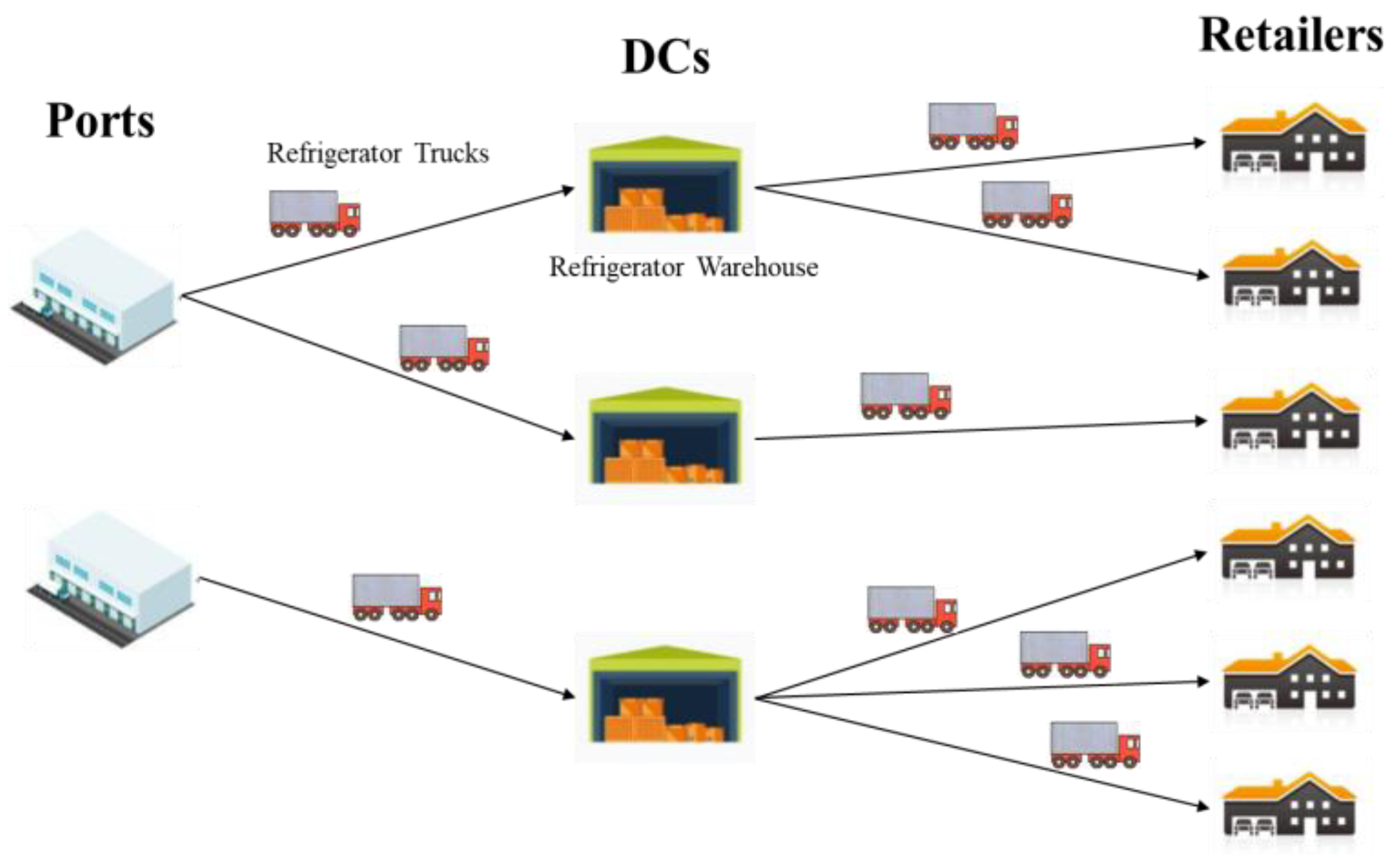
3.1. Problem Descriptions
The products of our research scope are fresh fruit, frozen meat, and frozen seafood, which are the most favorite imported products in China according to statistical reports [2]. They are all perishable and need to be stored and transported using refrigerated warehouses and vehicles at specific temperatures [3]. For example, the maximum temperature for frozen meat and frozen seafood is –18 °C, and the temperature range for most fresh fruit is 0–4 °C. It is reported that the cold chain of fresh products in China is mainly fulfilled by refrigerated warehouses and trucks, which cost a lot and cause environmental issues [41]. Therefore, our work in designing a cold supply chain network focuses on the complicated land distribution progress in China when products are imported from ports and transported to retailers at target cities. Consequently, a three-tier network involving three types of locations is investigated, as shown in Figure 1 and explained as follows.
Figure 1.
The schematic diagram of a cold chain network for imported fresh agri-products. DCs: distribution centers.
The first type of location is the port, which is usually known as the Free Trade Zone for importing fresh agri-products. Various fresh products from different countries are transported or stored at ports. After Customs Clearance, the products will then be transported to the second type of location, namely, DCs (distribution centers). DCs in the cold chain consist of refrigerated warehouses where fresh products can be temporarily stored, removed, and loaded, which is known as cross-docking. Consequently, DCs will incur a financial cost and cause carbon emissions due to the use of energy and operations. The last type of location is the retailers in the target cities, where various demands for the different fresh agri-products should be satisfied. The transportation between locations depends on refrigerated trucks. It is assumed that different products that require different refrigeration temperatures are transported by different vehicles. A distributor is faced with the problem of deciding which places should be selected as distribution centers and how to fulfill the demand of each of the retailers in order to balance between the minimum cost and the carbon emissions. Hereinafter, we use the terms inbound and outbound to represent transportation from ports to DCs and DCs to retailers, respectively.
A complete list of parameters and variables is given in Table 1. Preliminary work on assessing emissions is introduced as follows.
Table 1.
The definitions of the parameters and variables.
(1) Carbon Emissions of Transportation
There is no standard for the assessment of transportation-related carbon emissions. However, a general approach can be observed [5,42]. Accordingly, we consider three factors, namely, distance, outdoor ambient temperature, and the set point of refrigerator temperature regarding different types of products. The most comprehensive data that show the relationship between ambient temperatures, refrigeration temperatures, and vehicular GHG emissions are presented by Wu et al. [7]. It indicates clearly that higher ambient temperatures lead to higher energy consumption and, consequently, increased carbon emissions. Moreover, the set point of the refrigerator temperature has a negative correlation with carbon emissions as well.
In this paper, based on the published experimental data, an expression relating the ambient temperatures to CO2 emissions is derived. Let denote the unit carbon emission rate in traveling from port i to DC j for product u. Let and be the average annual temperature of ports and DCs, respectively. Then, the unit carbon emission rate is estimated as . Here, the average annual temperature of the two locations is used to estimate the overall temperature condition from port i to DC j. is a monotonic increasing function with the ambient temperature as well. Similarly, the value of , the unit carbon emission rate for transporting product u from DC j to retailer k, can be determined.
(2) Carbon Emissions of DCs
The carbon emissions of DCs in the cold chain are generated when maintaining refrigerated warehouses where the products are stored, removed, and loaded. Due to door openings; product removal/loading; and the heat conduction through doors, walls, roofs, and floors; the emission rate is positively correlated with the outdoor ambient temperature [4,6]. Consequently, the location of the DCs will affect the outdoor ambient temperature patterns, as well as the energy use and emissions, accordingly. Meneghetti and Monti [6] conducted research on the sustainable design of refrigerated automated food warehouses. They published the yearly cost, energy consumption, and emissions of warehouses based on reference cases from different locations with different temperature patterns. However, direct and general models to measure carbon emissions of DCs are rare. By combined use of the results and data from references [6,7], an expression for the carbon emission of DCs can be derived. Let be the average annual temperature of a potential DC; its carbon emission for a given period (for example, a year), , is estimated as ,where is a relationship between the carbon emission and average annual temperature, and can be formulated as a monotonic increasing function with .
3.2. Model Development
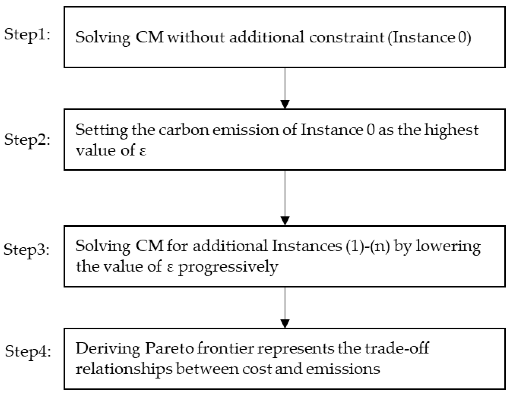
In order to balance between the financial and environmental indicators, a multi-objective mixed-integer linear program is formulated for the cold chain network design of imported fresh agri-products. The objective of the model is to minimize both the financial cost and the total carbon emissions. The complete model is given as follows and IM is used to denote this initial model.
IM:
s.t.
The first objective (OF1) in Equation (1) is the financial objective which is measured as the total cost including the following three parts: the overall transportation cost from ports to the DCs, the total transportation cost from the DCs to retailers, and the cost for opening and maintaining DCs. The second objective (OF2) in Equation (2) is the environmental objective and is measured as the total carbon emissions that consist of the following three parts: the total carbon emission for transporting products from ports to the DCs, the overall carbon emission for transporting products from DCs to retailers, and the fixed carbon emissions of DCs for a given time period (for example, a year).
Constraint (3) represents the supply capacity of each product from each port. Constraint (4) ensures that the demand from each retailer is satisfied. Constraint (5) guarantees the outbound flow must be no more than the inbound flow at each DC. Constraints (6) and (7) use a big number, M, to guarantee that only when a potential DC is selected will there be an inbound and outbound logistic flow associated with the DC. Constraints (8) and (9) ensure that the total number of selected DCs should follow some strategic requirement. Constraints (10) and (11) are for the non-negative and binary decision variables.
3.3. Model Solution
The ε-constraint method is used to solve the MOLP model; detailed principles of the method can be found elsewhere [8,43]. According to the ε-constraint method, the optimization progress of the two objectives is converted into optimizing the first objective (OF1) while formulating the second objective (OF2) as an additional constraint. In the CM (Converted Model), the formulation of the first objective (OF1) and the original Constraints (3)–(11) are in accordance with IM. The second objective (OF2) is converted into an additional constraint (Constraint (12)). Here, the left-hand side of the additional constraint (Constraint (12)) is equal to Constraint (2). Additionally, the right-hand side value of Equation (12) is ε, which represents the limit on the second objective (carbon emissions).
- CM: min OF1 (1)
- s.t.: Constraints (3)–(11);
A Pareto frontier that represents the correlation between the two objectives can be accordingly derived as shown in Figure 2. It is obtained by solving CM repeatedly for a set of instances. The initial instance (Instance 0) is generated by solving the objective value of OF1 according to the CM without the additional constraint (Constraint (12)). Then, using the results, the second objective (OF2)—carbon emissions of Instance 0—can be calculated and set as the highest value of ε. In order to generate a set of n instances, the value of ε is reduced progressively. Finally, by solving the CM with a set of n + 1 instances, the relationship of OF1 and OF2 can be obtained step by step; a Pareto frontier can then be obtained.
Figure 2.
The steps for deriving the Pareto frontier. CM: converted model.
4. Numerical Experiments
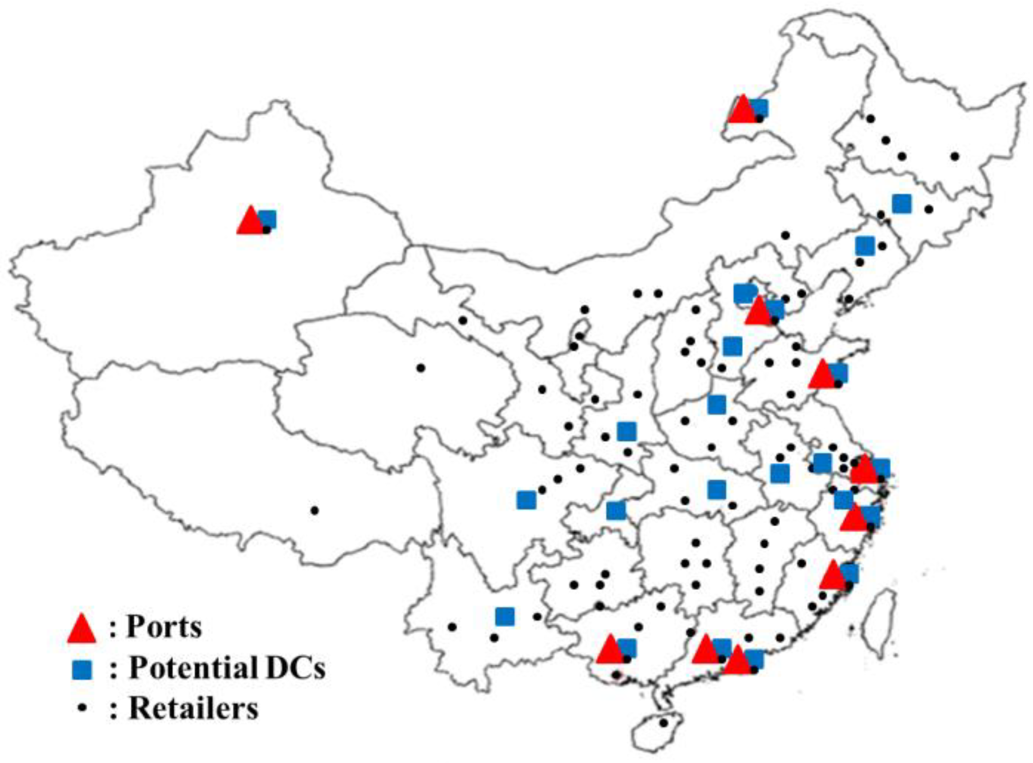
4.1. Data Collection
We implement the proposed multi-objective linear programming model using reference examples derived from facts and reports on imported fresh-agri products in China. The overview of the whole network that covers ports, potential DCs, and retailers is presented in Figure 3.
Figure 3.
The logistics network of imported fresh agri-products in China.
Ports: As shown in Figure 3, 10 importing ports were selected according to the report by the 21st Century Institute of Economic Research [44]. In particular, under the development of Belt and Road, the port of Nanning in the southeast of China and ports of Urumqi and Manchuria adjacent to Europe were selected due to the increasing demand for products from middle-south Asia and Europe. Detailed information of the ports can be found in Table A1 in Appendix A.
DCs: Twenty-three potential distribution centers were selected from metropolises and capitals of provinces where transport is convenient and the demand is high. Detailed information of the potential distribution centers can be found in Table A2 in Appendix A.
Retailers: One hundred retailers representing cities where the imported fresh agri-products are sold in a large amount (according to the statistics by iresearch) were selected [45]. We list the selected cities in Table A3 in Appendix A.
Temperatures and Distances: We used the average annual temperatures to represent the overall temperature patterns of each city; the data were gathered from websites focusing on the weather in China [46]. As for the distance between two locations, the route distances between them were gathered according to the digital map provided by Baidu [47]. The details are listed in Table A1, Table A2 and Table A3 in Appendix A.
Product Types: In the reference case, the most favorite agri-products were considered; these are grouped into two types, namely, fresh fruit and frozen food (such as frozen meat and frozen seafood). The storage temperatures for these two types of products were set as 0 °C and –18 °C, respectively [3,22].
Demand and Supply: The demand of each city and supply of each port are simulated by the following steps. According to demographic information [48], the cities are divided into three categories: big, medium, and small cities. For simplicity and without loss of generality, the demand of each city category is assumed to follow a uniform distribution. The distributions for each type of city are assumed to be U(4,000,000, 5,000,000), U(2,000,000, 3,000,000), and U(500,000, 1,000,000), respectively. By summing all the demands together, the overall supply can be obtained. Then, by splitting the overall supply, the supply of each port can be determined. Here, the published throughput data of each port [49] were used as the weight for splitting the overall supply for each port. The details can be found in Table A1 and Table A3 in Appendix A.
Carbon Emission Rate of Freight Transportation: The carbon emissions of transportation are caused by the consumption of fuel/energy [50]. According to the method presented by Defra [51,52], the emission rate e (kg CO2/kg·km) can be calculated by Equation (13), where L refers to the liters in fuel per kg·km (L/kg·km) and represents the fuel conversion factor (kg CO2/L). Here, we use 2.63 kg CO2/L for the fuel conversion factor [52].
The other required parameter for the formulation is the liters of fuel per kg·km of refrigerator trucks. Unfortunately, there is no direct data available. To determine this value, two parts of the fuel consumption were distinguished: (1) the fuel consumptions for the load and transport, , and (2) the fuel consumptions for the refrigerator under the vehicle, .
Generally speaking, the fuel consumption rates for inbound and outbound transportation are different because the inbound transportation is usually carried out by higher-payload vehicles [53]. Then, the data of fuel consumptions for load and transport published by Reference [5] were used to derive the fuel consumption for inbound and outbound transportation. As shown in Table 2, two types of vehicles—heavy goods vehicles with 24–40 tons and 12–24 tons of gross vehicle mass respectively (HGV-40, HGV-24)—were assumed to be used for inbound transport and outbound transport, respectively. Because the transportation is usually between cities, the vehicles are assumed to be with maximum payload. Then, the fuel consumption rates for the two transportations, and , are determined as 0.01427 L/ kg·km and 0.01958 L/ kg·km accordingly.
Table 2.
The fuel consumption data [5]. HGV-40: heavy goods vehicles with 24–40 tons gross vehicle mass; HGV-24: heavy goods vehicles with 12–24 tons gross vehicle mass.
The fuel consumption rate of refrigerators is mainly affected by outdoor ambient temperature patterns and the set point of refrigerator temperatures. According to the model proposed by Reference [7], the fuel consumption of refrigerators is presented in Equation (15).
Here, is the base value of fuel consumption for a typical refrigerator in a reference scenario. COP is the coefficient of performance of refrigerators with respect to the outside ambient temperatures and the refrigeration temperatures. A higher ambient temperature or a lower refrigeration temperature will lead to a smaller COP, resulting in greater energy consumption. Wu et al. [7] also published a variation to the COP with the ambient temperature at the refrigeration temperatures of 0 °C and –18 °C for the typical refrigerator type, Carrier Xarios 600, R410A, as shown in Figure 4. Here, the base fuel consumption per unit weight per unit distance, , is 3.6 × 10⁻⁶ L/kg·km. Based on the published data and Equation (15), we can derive the fuel consumption rate of a refrigerator at different ambient and refrigeration temperature conditions.
Figure 4.
The coefficient of performance (COP) variation with the ambient temperature at two refrigeration temperatures [7]. (Xarios 600, R410A, v = 21–70 km/h).
Cost Rate of Freight Transportation: In this research, the variable cost for the product transportation is considered as the fuel cost. Then, the unit cost of the inbound and outbound transportations is calculated by Equation (16), where L refers to the liters of fuel per kg·km (L/ kg·km) and represents the fuel price (yuan/L). The data of the price is obtained from the website of Oil Price in China and set to be 6.2 yuan/L [54]. Combined with Equations (14) and (15), the unit costs of the inbound and outbound transportations, and , can be estimated.
Carbon Emission Rate of DCs: The carbon emissions of a DC, , are estimated as , a monotonically increasing function with respect to the average temperature [4,6]. Few comprehensive datasets exist to show warehouse emissions, while the general relationship between the ambient temperature and emissions will not change (that is, the linear, concave, or convex relationship) [12]. Similarly, with Equation (13), the carbon emission of a warehouse can be formulated as Equation (17). Here, P represents the energy consumed by the warehouse within a given period (for example, a year) and without loss of generality, the energy of the warehouse is provided by electricity. is the carbon emissions factor for the electrical supply. According to the IEA report [55], the emission factor for China is 0.766 kg CO2/kWh.
Meneghetti and Monti [6] investigated the energy consumption of refrigerated warehouses at different places with different ambient temperature patterns. According to the published data by Reference [6], a linear function is used to approximate P as and the values of a and b are set as 2066.6 and 726,074.5, respectively.
Cost of DCs. The cost of DCs comprises the fixed cost for maintaining DCs and the variable cost for energy use. In reality, the fixed cost can hardly be found; thus, we approximated it as 1,000,000,000 yuan. For the energy cost, we calculated the amount of consumed electricity, P, as a multiple of the electricity price. Through the website of the National Energy Administration, we established that the price is 1.2 yuan/kWh [56].
A summary of the values of the parameters related to the cost and emissions is presented in Table A4 in Appendix A.
4.2. Analysis and Discussion
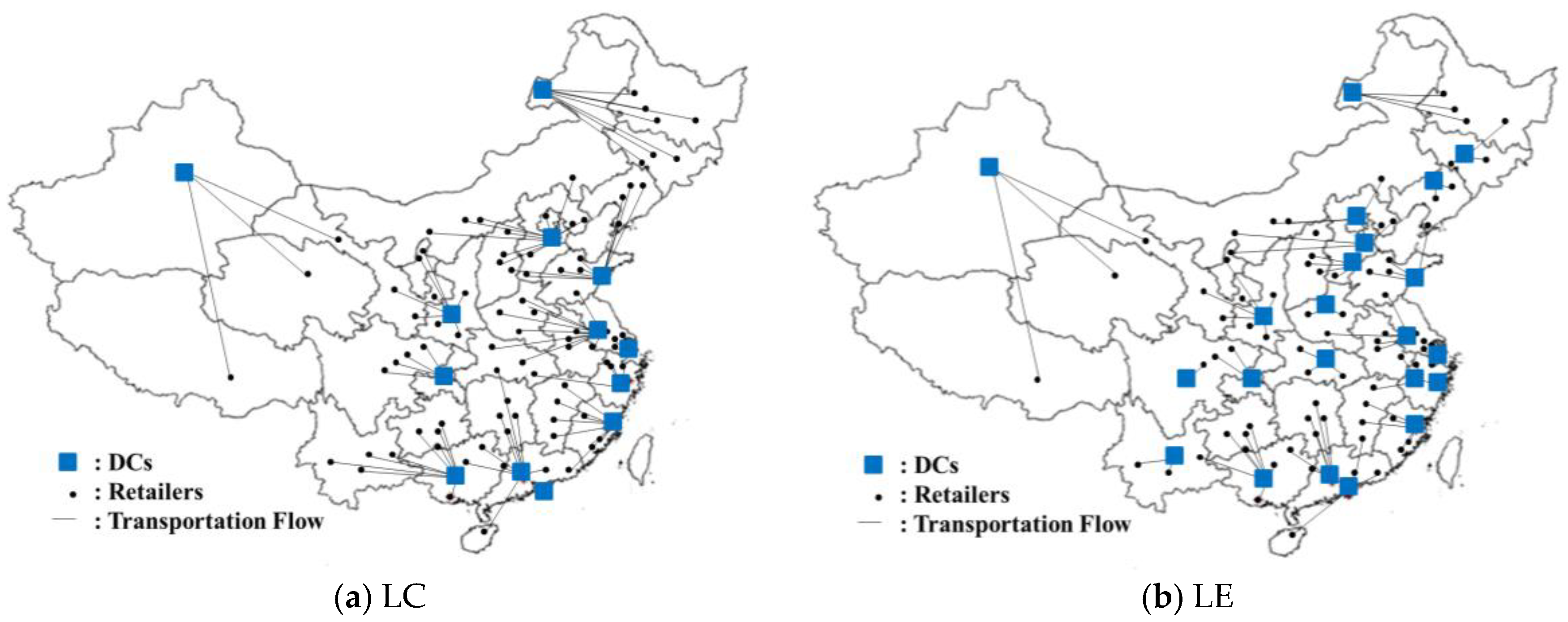
4.2.1. Solutions of the Two Base Scenarios with a Single Objective
The MOLP model was solved by the Cplex optimization solver. Two base scenarios with a single objective were defined as the lowest cost (LC) and lowest emission (LE). The summary of the results of the LC and LE cases is shown in Table 3 and the overall locations of DCs are presented in Figure 5a,b respectively. So as to not complicate the figure, the ports and transportation flow through ports to DCs are not shown. Through a quick comparison between LC and LE, the change of cost and emissions can be observed. The items for the cost and emissions are classified into three parts: inbound transportation, outbound transportation, and DC maintenance. The results show that the cost and emission items for inbound transportation and DCs are increasing in the LE case, while that of outbound transportation changes in the opposite way. However, the decreased emission for outbound transportation exceeds the increased amount of the inbound transportation and DCs. Thus, the overall emission of LE is the lowest. This is mainly because the total number of distribution centers under LE is much higher than that under LC. An increase in the DC numbers will shorten the distance from DCs to retailers sharply, which will decrease the correlated outbound transportation costs and emission. The results suggest that a distributed structure of the network is more conducive to reducing carbon emissions.
Table 3.
Summary results of two base cases.
Figure 5.
The locations of DCs for the two base cases.
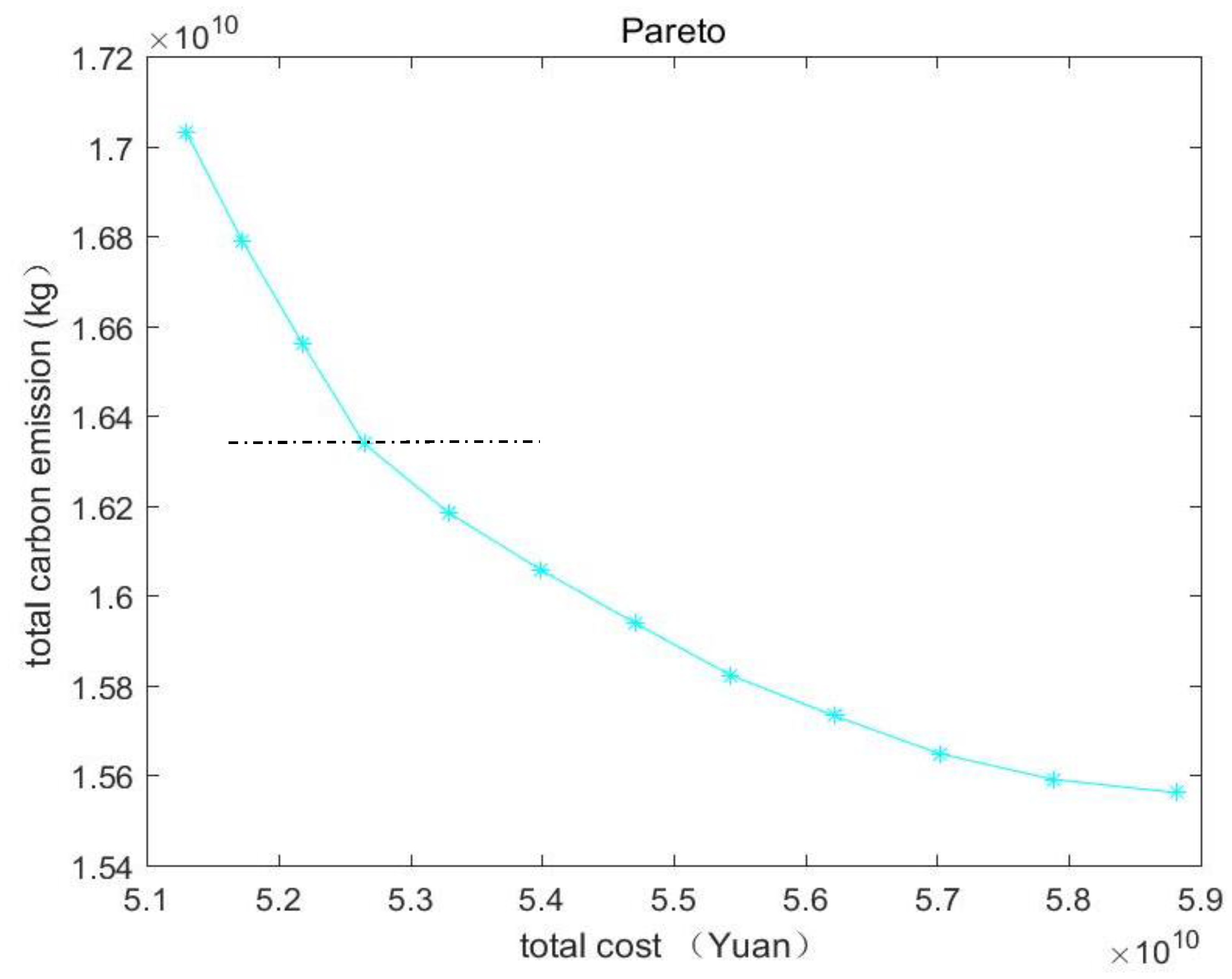
4.2.2. The Trade-Offs between the Two Objectives
In our problem, due to different locations of the DCs, trade-offs occur between the inbound transportation, outbound transportation, and DC maintenance. According to the base cases, 10 additional instances are generated by lowering the ε value from the highest emission level (emission of LC) to the lowest one (emission of LE) with an even interval. The trade-off between costs and emissions is shown in the derived Pareto frontier in Figure 6. The ends of the curve denote the cost and emission levels of the two base scenarios. The 10 additional scenarios are present on the curve. The shape of the Pareto frontier clearly shows that it costs more to get on the same portion of emission reduction. The cost and emission structure of each scenario and the features of their DCs are presented in Figure 7 and Table 4. The findings are as follows:
Figure 6.
The trade-offs between the total cost and carbon emissions.
Figure 7.
The cost and emission structure of each scenario on the Pareto frontier in Figure 6. IB: inbound; OB: outbound.
Table 4.
Number and the average temperature of DCs of each scenario on the Pareto frontier in Figure 6.
- (1)
- The main reason for emission reduction on the cold chain is because of the increase of DC numbers. When more DCs are selected, the distance of outbound transportation will sharply drop. Then, the emission items related to outbound transportation will decrease, which can compensate for the emission increase related to inbound transportation and DC maintenance.
- (2)
- By carefully comparing the average temperature of each DC as shown in Table 4, we can see that when the number of DCs is increased, the average temperatures of DCs increase accordingly. Meanwhile, when the number of DCs stays equal—for example, in Scenarios 3, 4, and 5—the average temperature declines, which can, in turn, reduce the overall carbon emissions. This explains the decline on the Pareto frontier at the Scenario 3 point. The number of DCs increases at a rate of 2 for Scenarios 1, 2, 3, and the LC scenario. Meanwhile, the number stays stable for Scenario 4. This means that the emission reductions of outbound transportation cannot cover the emission increase caused by opening a DC. Consequently, an emission reduction can be obtained by moving DCs to lower-temperature places, which consequently increases the transportation cost.
- (3)
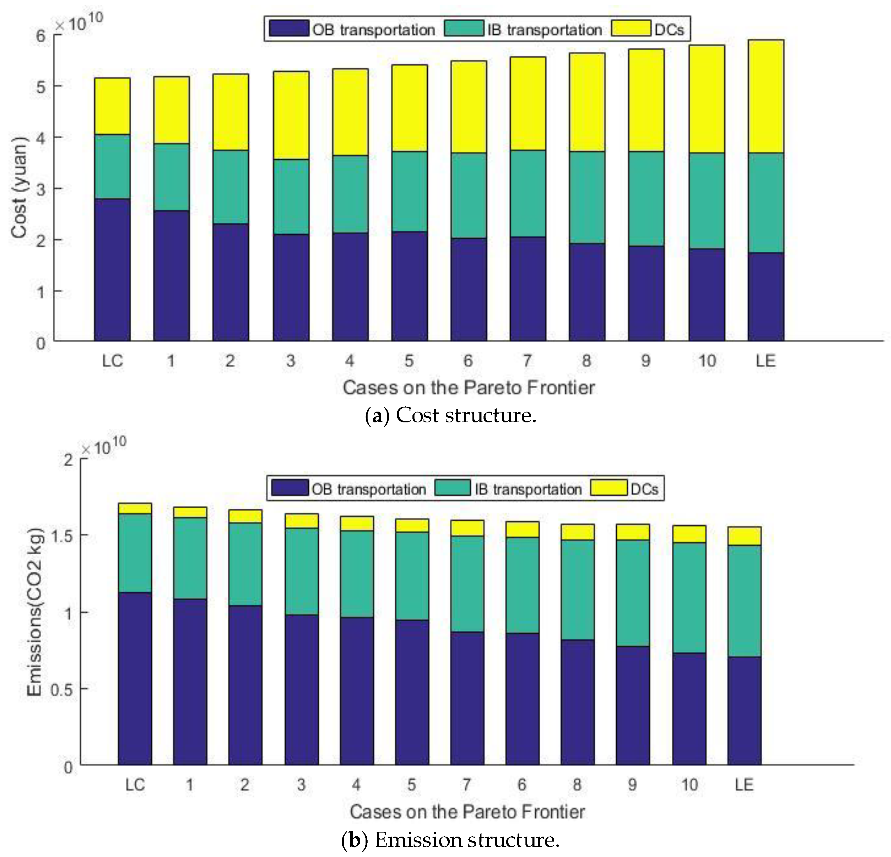
- The cost and emissions for inbound transportation and DC maintenance are positively related to the number of DCs, while the effect on outbound transportation is exactly the same in the opposite way. Moreover, the carbon emissions caused by transportation account for the largest share of the total emissions. This provides an important direction for the control of carbon emissions in cold supply chains.
5. Conclusions
In this study, we present a MOLP model for the green cold chain design problem for imported fresh agri-products in China. The distinguishing features of the proposed model lie in three aspects: (1) effects of outdoor ambient temperatures on emissions are considered; (2) the model can be applied to multiple highly perishable products required for different set-point temperatures; (3) it can cope with two competing goals—minimizing the total cost and carbon emissions. The model can aid strategic decisions on where distribution centers need to be located and how many of them are needed along with a cold chain, as well as support operational decisions on which route to choose in complicated networks. This model will have important applications in cold chain network design for perishable products under green considerations.
The MOLP model was solved using the ε-constraint method and verified by numerical experiments inspired by operating cases of imported fresh agri-products under the development of Belt and Road in China. The Pareto frontier represents the trade-off between the cost and emissions that has been obtained. Managerial insights can be derived from improving sustainability of the cold chain network. For example, how much additional cost would the company like to pay in order to reduce the emission level? Is there a need for the government to provide subsidies for sustainable cold chain design? The results obtained from the numerical analysis indicate that there are two main reasons for carbon emissions in the cold chain. The first one is the number of DCs, which can reduce emissions by shortening the travel distances between DCs and retailers. The average temperatures give another way of reducing emissions by moving DCs to cooler places to save on energy use. The computational experiments also show that emissions in transportation are a major part of the total emissions. It is appropriate to construct a cold chain with a distributed structure to reduce the transportation emissions. The method of enhancing the energy efficiency during transportation is important for controlling the emission level in green cold chain management.
There are several proposed future research areas that are extensions of the proposed method. Firstly, how to use the day-to-day temperature data instead of the average annual temperature for the decision-making is a direction to investigate in order to improve the precision of the proposed model. Secondly, the market of the imported fresh agri-products will have a lot of uncertainties because of customer preference for new products or market competition. How to design a flexible and sustainable cold chain would be an interesting research area as well. We leave this for future work.
Author Contributions
Y.F. and L.S. conceived the research idea and developed the model. Y.J. implemented and solved the model, while X.H. collected the data and presents the results. All four authors contributed to the wring and revising the manuscript.
Funding
This research was supported by National Natural Science Foundation of China [71601069], Humanity and Social Science Youth Foundation of Ministry of Education of China [17YJC630048], Social Science Planning Fund Program of Liaoning Province [L17BGL015], Natural Science Foundation of Jiangsu Province [BK20160742], the Fundamental Research Funds for the Central Universities [NAU: KYZ201663; NAU: SKTS2016038; NAU: SKYC2017007; NAU: SKYZ2017025], High Quality Engineering of Social Science Application Fund in Jiangsu [17SYC-026], and Project of Philosophy and Social Science Research in Colleges and Universities in Jiangsu [2017SJB0030].
Acknowledgments
The authors would like to thank the anonymous reviewers for their valuable and fruitful comments that improved the quality of this paper. We sincerely thank the editor and the referees for their constructive comments.
Conflicts of Interest
The authors declare no conflicts of interest.
Appendix A
Table A1.
The supply and temperatures of ports.
Table A1.
The supply and temperatures of ports.
| Ports | Manzhouli | Urumqi | Qingdao | Tianjin | Ningbo | Shanghai | Fuzhou |
| AAT (°C) | −1.2 | 8.4 | 12.3 | 13.8 | 16.6 | 17.6 | 21 |
| Supply of Fruit (ton) | 8000 | 10,000 | 32,000 | 26,000 | 52,000 | 47,000 | 23,000 |
| Supply of Frozen Product (ton) | 18,000 | 15,000 | 29,000 | 20,000 | 49,000 | 45,000 | 24,000 |
| Ports | Guangzhou | Nanning | Shenzhen | ||||
| AAT (°C) | 21.9 | 22.3 | 22.5 | ||||
| Supply of Fruit (ton) | 36,000 | 18,000 | 33,000 | ||||
| Supply of Frozen Product (ton) | 32,000 | 12,000 | 35,000 |
AAT: Average annual temperature; Sources: http://www.weather.com.cn [46].
Table A2.
The temperature of potential DCs.
Table A2.
The temperature of potential DCs.
| Potential DCs | Manzhouli | Changchun | Urumqi | Shenyang | Qingdao | Beijing | Tianjin |
| AAT (°C) | −1.2 | 6.6 | 8.4 | 8.8 | 12.3 | 13.8 | 13.8 |
| Potential DCs | Shijiazhuang | Kunming | Nanjing | Xi'an | Zhengzhou | Ningbo | Chengdu |
| AAT (°C) | 14.6 | 15.0 | 15.1 | 15.8 | 16.4 | 16.6 | 16.8 |
| Potential DCs | Hefei | Wuhan | Shanghai | Hangzhou | Chongqing | Fuzhou | Guangzhou |
| AAT (°C) | 17.0 | 17.3 | 17.6 | 18.2 | 19.5 | 21.0 | 21.9 |
| Potential DCs | Nanning | Shenzhen | |||||
| AAT (°C) | 22.3 | 22.5 |
AAT: Average annual temperature; Sources: http://www.weather.com.cn [46].
Table A3.
The temperatures and demand of retailers.
Table A3.
The temperatures and demand of retailers.
| Retailers | Manzhouli | Jiamusi | Qiqihar | Chifeng | Harbin | Jilin | Daqing |
|---|---|---|---|---|---|---|---|
| AAT (°C) | −1.2 | 3.0 | 3.2 | 3.5 | 3.5 | 3.9 | 4.2 |
| Demand of Fruit (ton) | 2511 | 2524 | 1009 | 2042 | 1578 | 1025 | 2196 |
| Demand of Frozen Product (ton) | 1674 | 1803 | 1442 | 1856 | 3155 | 1025 | 1464 |
| Retailers | Hohhot | Siping | Datong | Changchun | Fushun | Jiuquan | Zhangzhou |
| AAT (°C) | 4.3 | 5.9 | 6.4 | 6.6 | 6.6 | 6.6 | 6.7 |
| Demand of Fruit (ton) | 1033 | 2363 | 2369 | 3483 | 1312 | 2015 | 1505 |
| Demand of Frozen Product (ton) | 1475 | 1969 | 1974 | 3166 | 1312 | 1832 | 1505 |
| Retailers | Baotou | Lhasa | Urumqi | Yinchuan | Anshan | Shizuishan | Shenyang |
| AAT (°C) | 7.2 | 7.4 | 8.4 | 8.5 | 8.5 | 8.6 | 8.8 |
| Demand of Fruit (ton) | 2240 | 1766 | 1896 | 2449 | 1062 | 1354 | 2215 |
| Demand of Frozen Product (ton) | 1493 | 1766 | 1264 | 3061 | 1327 | 1504 | 3691 |
| Retailers | Pingliang | Yan'an | Taiyuan | Wuhai | Qinhuangdao | Yangquan | Lanzhou |
| AAT (°C) | 9.0 | 9.1 | 9.5 | 9.6 | 10.0 | 10.0 | 10.3 |
| Demand of Fruit (ton) | 1959 | 1122 | 4036 | 989 | 1422 | 2209 | 3830 |
| Demand of Frozen Product (ton) | 1306 | 1603 | 3363 | 1977 | 1580 | 1699 | 3482 |
| Retailers | Dalian | Tongchuan | Tianshui | Xianyang | Qingdao | Tangshan | Kaifeng |
| AAT (°C) | 10.5 | 10.6 | 11.0 | 11.1 | 12.3 | 12.5 | 12.5 |
| Demand of Fruit (ton) | 3020 | 2513 | 864 | 1952 | 4763 | 923 | 1216 |
| Demand of Frozen Product (ton) | 3020 | 1933 | 1440 | 1627 | 3664 | 1846 | 1216 |
| Retailers | Dongying | Zibo | Liupanshui | Beijing | Tianjin | Jinan | Handan |
| AAT (°C) | 12.8 | 13.3 | 13.5 | 13.8 | 13.8 | 13.8 | 14.0 |
| Demand of Fruit (ton) | 1579 | 1686 | 1683 | 4490 | 3636 | 4190 | 2356 |
| Demand of Frozen Product (ton) | 1435 | 1297 | 1870 | 7484 | 7271 | 3809 | 1812 |
| Retailers | Anshun | Zaozhuang | Qujing | Luoyang | Shijiazhuang | Huzhou | Luohe |
| AAT (°C) | 14.0 | 14.5 | 14.5 | 14.5 | 14.6 | 14.7 | 14.7 |
| Demand of Fruit (ton) | 1123 | 1817 | 1543 | 1554 | 1841 | 3951 | 2258 |
| Demand of Frozen Product (ton) | 1871 | 1817 | 1102 | 1036 | 3069 | 3592 | 1882 |
| Retailers | Kunming | Nanjing | Bengbu | Zunyi | Guiyang | Changzhou | Wuhu |
| AAT (°C) | 15.0 | 15.1 | 15.1 | 15.1 | 15.3 | 15.5 | 15.5 |
| Demand of Fruit (ton) | 2971 | 2494 | 2064 | 1216 | 3934 | 3991 | 2297 |
| Demand of Frozen Product (ton) | 3301 | 3563 | 1474 | 1216 | 3278 | 3070 | 1641 |
| Retailers | Baoshan | Zhenjiang | Suzhou | Xi'an | Jiaxing | Mianyang | Deyang |
| AAT (°C) | 15.5 | 15.6 | 15.7 | 15.8 | 15.9 | 16.0 | 16.0 |
| Demand of Fruit (ton) | 727 | 4371 | 3548 | 5298 | 2694 | 822 | 1735 |
| Demand of Frozen Product (ton) | 1212 | 3362 | 3225 | 3784 | 3367 | 1643 | 1446 |
| Retailers | Fuyang | Guangyuan | Xiangtan | Wuxi | Zhengzhou | Huainan | Jiujiang |
| AAT (°C) | 16.0 | 16.1 | 16.1 | 16.2 | 16.4 | 16.5 | 16.5 |
| Demand of Fruit (ton) | 1262 | 1681 | 1980 | 4801 | 2484 | 2016 | 1229 |
| Demand of Frozen Product (ton) | 1578 | 1681 | 1320 | 3693 | 3105 | 1440 | 1229 |
| Retailers | Ningbo | Chengdu | Yichang | Hefei | Zhuzhou | Huang Shi | Changsha |
| AAT (°C) | 16.6 | 16.8 | 16.9 | 17.0 | 17.0 | 17.0 | 17.2 |
| Demand of Fruit (ton) | 10910 | 10445 | 1250 | 1824 | 1678 | 1798 | 11,634 |
| Demand of Frozen Product (ton) | 7793 | 7461 | 1389 | 3648 | 1291 | 1798 | 7756 |
| Retailers | Wuhan | Nanchang | Shanghai | Hengyang | Hangzhou | Sanming | Ji'an |
| AAT (°C) | 17.3 | 17.4 | 17.6 | 18.0 | 18.2 | 18.2 | 18.5 |
| Demand of Fruit (ton) | 6421 | 4719 | 4225 | 1128 | 7858 | 2209 | 1732 |
| Demand of Frozen Product (ton) | 7134 | 3146 | 7041 | 1611 | 7858 | 1699 | 1924 |
| Retailers | Liuzhou | Ganzhou | Guilin | Chongqing | Yuxi | Shantou | Quanzhou |
| AAT (°C) | 18.8 | 18.8 | 19.3 | 19.5 | 19.8 | 20.0 | 20.2 |
| Demand of Fruit (ton) | 974 | 1495 | 4565 | 5977 | 1882 | 5179 | 1547 |
| Demand of Frozen Product (ton) | 1218 | 1359 | 3804 | 7471 | 1568 | 3984 | 1547 |
| Retailers | Fuzhou | Xiamen | Zhangzhou | Guangzhou | Huizhou | Nanning | Shenzhen |
| AAT (°C) | 21.0 | 21.0 | 21.4 | 21.9 | 22.0 | 22.3 | 22.5 |
| Demand of Fruit (ton) | 3108 | 4938 | 520 | 10,641 | 2256 | 2775 | 4490 |
| Demand of Frozen Product (ton) | 3453 | 3292 | 1039 | 7601 | 1880 | 3469 | 7483 |
| Retailers | North Sea | Haikou | |||||
| AAT (°C) | 22.9 | 24.2 | |||||
| Demand of Fruit (ton) | 2100 | 1443 | |||||
| Demand of Frozen Product (ton) | 1750 | 1443 |
AAT: Average annual temperature; Sources: http://www.weather.com.cn [46], https://map.baidu.com/ [47].
Table A4.
Summary of values or estimations of parameters related to cost and emissions.
Table A4.
Summary of values or estimations of parameters related to cost and emissions.
| Parameters | Values/Estimations | Sources |
|---|---|---|
| Fuel conversion factor | 2.63 kg CO2/L | https://www.gov.uk/government/uploads/system/uploads/attachment_data/file/69568/pb13792-emission-factor-methodologypaper-120706.pdf [52] |
| Fuel consumption rate for inbound transportation | 0.01427 L/kg·km | Kellner and Igl (2015) [5] |
| Fuel consumption rate for outbound transportation | 0.01958 L/kg·km | Kellner and Igl (2015) [5] |
| Base value of fuel consumption of refrigerators | 3.6 × 10⁻⁶ L/kg·km | Wu et al. (2013) [7] |
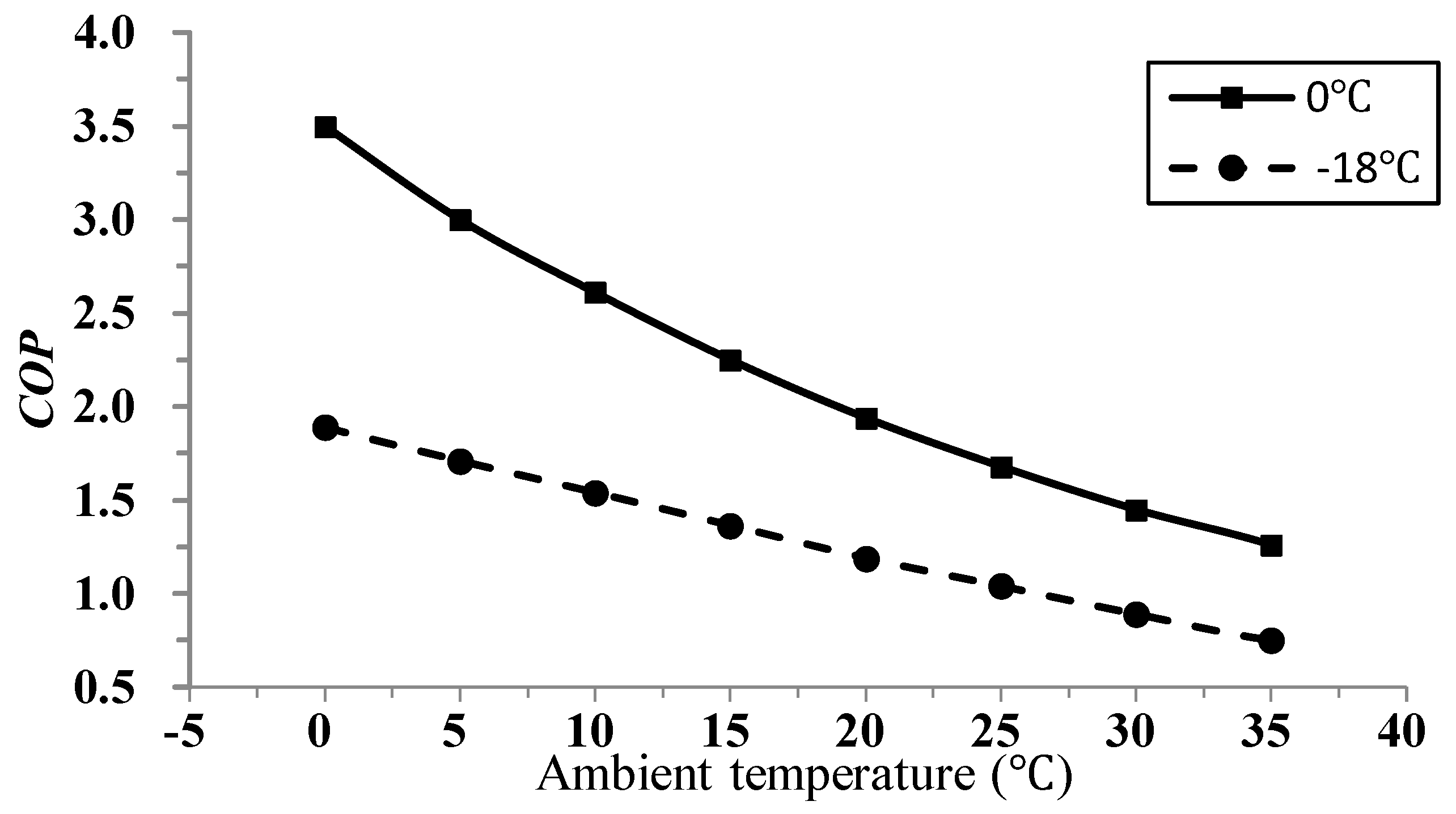
| Coefficient of performance of refrigerators | Data according to Figure 4 | Wu et al. (2013) [7] |
| Fuel price | 6.2 yuan/L [54] | http://youjia.chemcp.com [54] |
| Emission factor of electricity | 0.766 kg CO2/kWh | http://www.iea.org/publications/freepublications/publication/name,32870,en.html [55] |
| Fixed cost for maintaining DCs | 1,000,000,000 yuan | Assumption |
| Electricity price | 1.2 yuan/kWh | http://www.nea.gov.cn/ [56] |
References
- United Nations Development Programme in China (UNDP). Belt and Road Initiative. Available online: http://www.cn.undp.org/content/china/en/home/belt-and-road.html (accessed on 5 December 2017).
- Reports on Chinese Dinner Consumption Trend in 2018. Available online: http://www.cbndata.com/report/551/detail?isReading=report&page=1 (accessed on 20 January 2018).
- Coulomb, D. Refrigeration and cold chain serving the global food industry and creating a better future: Two key IIR challenges for improved health and environment. Trends Food Sci. Technol. 2008, 19, 413–417. [Google Scholar] [CrossRef]
- James, S.J.; James, C.; Evans, J.A. Modelling of food transportation systems—A review. Int. J. Refrigeration 2006, 29, 947–957. [Google Scholar] [CrossRef]
- Kellner, F.; Igl, J. Greenhouse gas reduction in transport: Analyzing the carbon dioxide performance of different freight forwarder networks. J. Clean. Prod. 2015, 99, 177–191. [Google Scholar] [CrossRef]
- Meneghetti, A.; Monti, L. Greening the food supply chain: An optimisation model for sustainable design of refrigerated automated warehouses. Int. J. Prod. Res. 2015, 53, 6567–6587. [Google Scholar] [CrossRef]
- Wu, X.; Hu, S.; Mo, S. Carbon footprint model for evaluating the global warming impact of food transport refrigeration systems. J. Clean. Prod. 2013, 54, 115–124. [Google Scholar] [CrossRef]
- Soysal, M.; Bloemhof-Ruwaard, J.M.; van der Vorst, J.G.A.J. Modelling food logistics networks with emission considerations: The case of an international beef supply chain. Int. J. Prod. Econ. 2014, 152, 57–70. [Google Scholar] [CrossRef]
- Eskandarpour, M.; Dejax, P.; Miemczyk, J.; Pétona, O. Sustainable supply chain network design: An optimization-oriented review. Omega 2015, 54, 11–32. [Google Scholar] [CrossRef]
- Arıkan, E.; Fichtinger, J.; Ries, J.M. Impact of transportation lead-time variability on the economic and environmental performance of inventory systems. Int. J. Prod. Econ. 2014, 157, 279–288. [Google Scholar] [CrossRef]
- Lee, K.H.; Cheong, I.M. Measuring a carbon footprint and environmental practice: The case of Hyundai Motors Co.(HMC). Ind. Manag. Data Syst. 2011, 111, 961–978. [Google Scholar] [CrossRef]
- Elhedhli, S.; Merrick, R. Green supply chain network design to reduce carbon emissions. Transp. Res. Part D Transp. Environ. 2012, 17, 370–379. [Google Scholar] [CrossRef]
- Benjaafar, S.; Li, Y.; Daskin, M. Carbon footprint and the management of supply chains: Insights from simple models. IEEE Trans. Autom. Sci. Eng. 2013, 10, 99–116. [Google Scholar] [CrossRef]
- Gallo, A.; Accorsi, R.; Baruffaldi, G.; Manzini, R. Designing Sustainable Cold Chains for Long-Range Food Distribution: Energy-Effective Corridors on the Silk Road Belt. Sustainability 2017, 9, 2044. [Google Scholar] [CrossRef]
- Lee, D.H.; Dong, M.; Bian, W. The design of sustainable logistics network under uncertainty. Int. J. Prod. Econ. 2010, 128, 159–166. [Google Scholar] [CrossRef]
- Pishvaee, M.S.; Razmi, J. Environmental supply chain network design using multi-objective fuzzy mathematical programming. Appl. Math. Model. 2012, 36, 3433–3446. [Google Scholar] [CrossRef]
- Tozzi, M.; Corazza, M.V.; Musso, A. Urban goods movements in a sensitive context: The case of Parma. Res. Transp. Bus. Manag. 2014, 11, 134–141. [Google Scholar] [CrossRef]
- Borodin, V.; Bourtembourg, J.; Hnaien, F.; Labadiec, N. Handling uncertainty in agricultural supply chain management: A state of the art. Eur. J. Oper. Res. 2016, 254, 348–359. [Google Scholar] [CrossRef]
- Tzamalis, P.G.; Panagiotakos, D.B.; Drosinos, E.H. A ‘best practice score’ for the assessment of food quality and safety management systems in fresh-cut produce sector. Food Control 2016, 63, 179–186. [Google Scholar] [CrossRef]
- Validi, S.; Bhattacharya, A.; Byrne, P.J. A case analysis of a sustainable food supply chain distribution system—A multi-objective approach. Int. J. Prod. Econ. 2014, 152, 71–87. [Google Scholar] [CrossRef]
- Brandenburg, M.; Govindan, K.; Sarkis, J.; Seuringa, S. Quantitative models for sustainable supply chain management: Developments and directions. Eur. J. Oper. Res. 2014, 233, 299–312. [Google Scholar] [CrossRef]
- Panozzo, G.; Cortella, G. Standards for transport of perishable goods are still adequate? Connections between standards and technologies in perishable foodstuffs transport. Food Sci. Technol. 2008, 19, 432–440. [Google Scholar] [CrossRef]
- Yang, S.; Xiao, Y.; Zheng, Y.; Liu, Y. The Green Supply Chain Design and Marketing Strategy for Perishable Food Based on Temperature Control. Sustainability 2017, 9, 1511. [Google Scholar] [CrossRef]
- Pipatprapa, A.; Huang, H.H.; Huang, C.H. A novel environmental performance evaluation of Thailand’s food industry using structural equation modeling and fuzzy analytic hierarchy techniques. Sustainability 2016, 8, 246. [Google Scholar] [CrossRef]
- Gwanpua, S.G.; Verboven, P.; Leducq, D.; Brownc, T.; Verlindend, B.E.; Bekelea, E.; Aregawia, W.; Evansc, J.; Fosterc, A.; Duretb, S.; et al. The FRISBEE tool, a software for optimising the trade-off between food quality, energy use, and glob al warming impact of cold chains. J. Food Eng. 2015, 148, 2–12. [Google Scholar] [CrossRef]
- Strotmann, C.; Göbel, C.; Friedrich, S.; Kreyenschmidt, J.; Ritter, G.; Teitscheid, P. A participatory approach to minimizing food waste in the food industry—A manual for managers. Sustainability 2017, 9, 66. [Google Scholar] [CrossRef]
- Bosona, T.G.; Gebresenbet, G. Cluster building and logistics network integration of local food supply chain. Biosyst. Eng. 2011, 108, 293–302. [Google Scholar] [CrossRef]
- Amorim, P.; Almada-Lobo, B. The impact of food perishability issues in the vehicle routing problem. Comput. Ind. Eng. 2014, 67, 223–233. [Google Scholar] [CrossRef]
- Wang, S.; Tao, F.; Shi, Y.; Wen, H. Optimization of vehicle routing problem with time windows for cold chain logistics based on carbon tax. Sustainability 2017, 9, 694. [Google Scholar] [CrossRef]
- Jindal, A.; Sangwan, K.S. Closed loop supply chain network design and optimisation using fuzzy mixed integer linear programming model. Int. J. Prod. Res. 2014, 52, 4156–4173. [Google Scholar] [CrossRef]
- Hasani, A.; Khosrojerdi, A. Robust global supply chain network design under disruption and uncertainty considering resilience strategies: A parallel memetic algorithm for a real-life case study. Transp. Res. Part E Logist. Transp. Rev. 2016, 87, 20–52. [Google Scholar] [CrossRef]
- Rezaee, A.; Dehghanian, F.; Fahimnia, B.; Beamon, B. Green supply chain network design with stochastic demand and carbon price. Ann. Oper. Res. 2017, 250, 463–485. [Google Scholar] [CrossRef]
- Farahani, R.Z.; Rezapour, S.; Drezner, T.; Fallahd, S. Competitive supply chain network design: An overview of classifications, models, solution techniques and applications. Omega 2014, 45, 92–118. [Google Scholar] [CrossRef]
- Govindan, K.; Fattahi, M.; Keyvanshokooh, E. Supply chain network design under uncertainty: A comprehensive review and future research directions. Eur. J. Oper. Res. 2017, 263, 108–141. [Google Scholar] [CrossRef]
- Srivastava, S.K. Network design for reverse logistics. Omega 2008, 36, 535–548. [Google Scholar] [CrossRef]
- Chaabane, A.; Ramudhin, A.; Paquet, M. Design of sustainable supply chains under the emission trading scheme. Int. J. Prod. Econ. 2012, 135, 37–49. [Google Scholar] [CrossRef]
- Akgul, O.; Shah, N.; Papageorgiou, L.G. An optimisation framework for a hybrid first/second generation bioethanol supply chain. Comput. Chem. Eng. 2012, 42, 101–114. [Google Scholar] [CrossRef]
- Bortolini, M.; Faccio, M.; Ferrari, E.; Gamberib, M.; Pilatib, F. Fresh food sustainable distribution: Cost, delivery time and carbon footprint three-objective optimization. J. Food Eng. 2016, 174, 56–67. [Google Scholar] [CrossRef]
- Osvald, A.; Stirn, L.Z. A vehicle routing algorithm for the distribution of fresh vegetables and similar perishable food. J. Food Eng. 2008, 85, 285–295. [Google Scholar] [CrossRef]
- Coskun, S.; Ozgur, L.; Polat, O.; Gungor, A. A model proposal for green supply chain network design based on consumer segmentation. J. Clean. Prod. 2016, 110, 149–157. [Google Scholar] [CrossRef]
- Analysis on the Development Prospect of China’s Cold Chain Logistics Industry in 2017. Available online: http://www.chyxx.com/industry/201709/560686.html (accessed on 19 January 2018).
- Olsthoorn, X.; Tyteca, D.; Wehrmeyer, W.; Wagnerc, M. Environmental indicators for business: A review of the literature and standardisation methods. J. Clean. Prod. 2001, 9, 453–463. [Google Scholar] [CrossRef]
- Andersson, J. A Survey of Multi-objective Optimization in Engineering Design; Department of Mechanical Engineering, Linktjping University: Linköping, Sweden, 2000. [Google Scholar]
- Eating on Chinese New Year—Report on Consumption Trends of E-Commerce for Fresh Produce. Available online: http://www.sohu.com/a/126521289_476012 (accessed on 28 October 2017).
- Insights of E-Commerce for China’s Fresh Produce in 2018. Available online: http://report.iresearch.cn/report/201801/3123.shtml (accessed on 10 February 2018).
- Weather of China. Available online: http://www.weather.com.cn (accessed on 11 December 2017).
- Baidu Map. Available online: https://map.baidu.com/ (accessed on 12 December 2017).
- National Bureau of Statistics of China. Available online: http://www.stats.gov.cn/tjsj/ (accessed on 1 February 2018).
- Chinaports. Available online: http://www.chinaports.com/thruput (accessed on 2 February 2018).
- McKinnon, A.C.; Piecyk, M.I. Measurement of CO2 emissions from road freight transport: A review of UK experience. Energy Policy 2009, 37, 3733–3742. [Google Scholar] [CrossRef]
- DEFRA (Department for Environment, Food and Rural Affairs). Greenhouse Gas Conversion Factors for Company Reporting. 2012. Available online: https://www.gov.uk/government/uploads/system/uploads/attachment_data/file/69555/pb13773-ghg-conversionfactors2012.xls (accessed on 27 January 2018).
- DEFRA (Department for Environment, Food and Rural Affairs). Guidelines to Defra/DECC’s GHG Conversion Factors for Company Reporting, Methodology Paper for Emission Factors. 2012. Available online: https://www.gov.uk/government/uploads/system/uploads/attachment_data/file/69568/pb13792-emission-factor-methodologypaper-120706.pdf (accessed on 27 January 2018).
- Tsao, Y.C.; Lu, J.C. A supply chain network design considering transportation cost discounts. Transp. Res. Part E Logist. Transp. Rev. 2012, 48, 401–414. [Google Scholar] [CrossRef]
- Oil Price in China. Available online: http://youjia.chemcp.com (accessed on 1 March 2018).
- International Energy Agency (IEA). CO2 Emissions from Fuel Combustion—Highlights. 2012. Available online: http://www.iea.org/publications/freepublications/publication/name,32870,en.html (accessed on 27 January 2018).
- National Energy Administration. Available online: http://www.nea.gov.cn/ (accessed on 8 March 2018).
© 2018 by the authors. Licensee MDPI, Basel, Switzerland. This article is an open access article distributed under the terms and conditions of the Creative Commons Attribution (CC BY) license (http://creativecommons.org/licenses/by/4.0/).