Abstract
Intervening in the built environment is a key way for land-use and transport planning and related policies to promote low-carbon development and low-carbon travel. It is of significance to explore and recognize the actual impact of the neighborhood built environment on travel-related CO2 emissions. This study calculated the CO2 emissions from four purposes of trips, which were within the urban region, using Travel O-D Point Intelligent Query System (TIQS) and 1239 residents’ travel survey questionnaires from 15 neighborhoods in Guangzhou. It measured the direct and indirect effects of built environments on CO2 emissions from different purposes of trips by developing structural equation models (SEMs). The results showed that for different purposes of trips, the effects of the neighborhood built environments on CO2 emissions were inconsistent. Almost all built environment elements had significant total effects on CO2 emissions, which were mainly indirect effects through mediators such as car ownership and trip distance, then affecting CO2 emissions indirectly. Most of the direct effects of neighborhood built environments on CO2 emissions were not significant, especially those from non-commuting trips. These findings suggest that in the process of formulating low-carbon oriented land-use and transport planning and policies, the indirect effects of the built environments should not be ignored, and the differences of the effects of the neighborhood built environments among different purposes of the trip should be fully considered.
1. Introduction
The transportation sector is the world’s second largest unsustainable energy user and contributor to carbon emissions, contributing 23.31% of global carbon dioxide (CO2) emissions in 2014 [1]. Regarded as the most difficult sector in which to achieve carbon reduction, it has the fastest growth rate of CO2 emissions and its global share is projected to rise to 30–50% by 2050 [2,3,4]. China surpassed the United States in 2007 and became the country with the largest total CO2 emissions in the world [5]. Over the past two decades, China’s urban development patterns have continued along the path of suburbanization and decentralized development, characteristic of the U.S.’s urban spread in the second half of the twentieth century. In the process of rapid urban expansion, the spread pattern of low density, decentralized development, and segregation of land-use has appeared in the urban fringe areas, which has greatly increased the distance of residents’ travel and the use of cars [6,7]. In this context, private car ownership in China has expanded rapidly, with 123.39 million in 2014, and the average annual growth rate was as high as 23.26% from 1985 to 2014. With the continuous development of the economy and more private cars, China’s carbon emissions from transportation will continue to grow [8].
Although the transportation sector is a large and diverse sector that includes air, land, and water transport, and the movement of both passengers and freight, people’s daily travel by passenger vehicles is the primary source of CO2 emissions [9]. Over the past two to three decades, numerous studies have examined the relationship between the built environment and travel behavior [10,11,12,13], focusing on trip frequencies, trip lengths, mode choices or modal splits, and person miles traveled (PMT), vehicle miles traveled (VMT), or vehicle hours traveled (VHT) [14,15]. However, little attention has been paid to travel-related carbon emissions, which can also be regarded as a travel behavior or an outcome of travel behavior [16,17]. Macro-level studies on CO2 emissions from transport have mainly explored the influencing factors based on the aggregate data of country, region, or city, using decomposition methods [18,19,20,21], scenario analysis [22,23,24], panel data models [8], and Data Envelopment Analysis (DEA) models [25,26,27]. They have seldom examined the effects of urban forms or built environments on transport-related CO2 emissions. Most studies on the neighborhood/local level have used questionnaires and disaggregate methods to investigate the impact of socio-demographics and built environments on residents’ travel behavior and its related CO2 emissions. Some research has focused on quantifying the effects of residents’ socio-demographic attributes on travel-related CO2 emissions and neglected to analyze the effects of built environment factors [28,29,30,31]. Others have primarily measured the direct effects of the built environment on travel-related CO2 emissions with case studies of cities in North America, Europe, and Oceania [28,32,33,34], but ignored the indirect effects of the built environment, which ultimately affects CO2 emissions through intermediary factors. Furthermore, they did not examine the differences in the effects of the built environments on CO2 emissions in terms of different purposes of trips [17,35,36].
In this paper, taking Guangzhou as an example, we measured the direct and indirect effects of neighborhood built environments on CO2 emissions from four purposes of trips based on survey data and structural equation modeling. It aimed to address the following two research questions: (1) How does the neighborhood built environment affect the travel-related CO2 emissions of residents? For example, do they affect CO2 emissions directly or indirectly by affecting other mediating variables?; (2) For different purposes of trips, are there any differences in the effects of neighborhood built environment elements on CO2 emissions?
The rest of this paper is organized as follows. Section 2 introduces the methodology and data used in the analysis. Section 3 examines the estimation results of the models and analyzes the direct and indirect effects of neighborhood built environments on travel-related CO2 emissions. Section 4 summarizes the primary conclusions and policy implications of the study.
2. Methodology and Data
2.1. Study Area and Neighborhoods Surveyed
This paper takes Guangzhou as the study area. It is the largest city in southern China and covers an area of 3647.43 km2 and includes 2055 neighborhoods. Its total population was 14.04 million in 2016. In order to select the survey neighborhoods, we first used GIS technology to measure the built environment for all these 2055 neighborhoods, including the following six criteria: the distance to city public centers (DTC), residential density (RD), land-use mix (LUM), bus stop density (BSD), metro station density (MSD), and road network density (RND). Specifically, the distance to city public centers was measured through the average Euclidean distance from the center of the neighborhood to 16 urban public centers of different types. The residential density was calculated by dividing the neighborhood population by the area of the neighborhood. The land-use mix was calculated by methods similar to those used in previous studies [37,38] with 13 types of points of interest (POIs). The bus stop density and the metro station density were obtained by estimating the bus stop vector data and the metro station vector data, respectively, using the kernel density method. The road network density was measured by the method of line density with the road network vector data. And then, to ensure the statistical significance of the model fit, we specifically chose neighborhoods with large differences in the built environment to conduct the survey. Eventually, 15 neighborhoods from 7 districts were selected. They are Fuli (FL), Wuyang (WY), Yijingcuiyuan (YJCY), Guangdahuayuan (GDHY), Fangcaoyuan (FCY), Junjinghuayuan (JJHY), Zhonghaikangcheng (ZHKC), Huiqiaoxincheng (HQXC), Fulicheng (FLC), Jinbi (JB), Wankehuayuan (WKHY), Luoxixincheng (LXXC), Lijianghuayuan (LJHY), Qifuxincun (QFXC), and Dongyi (DY) (Figure 1a). In the scatter plot and the fitting curve between the built environment elements of these neighborhoods, almost all their confidence ellipses have a larger area, which indicates that there are significant differences in the built environment elements between the surveyed neighborhoods (Figure 1b).
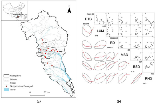
Figure 1.
(a) The spatial distribution of the neighborhoods surveyed; (b) the scatter plots and fitting curves between built environment elements.
2.2. Survey Data
A pre-survey exercise was conducted in March 2015. After feedback and refinement, the formal survey began in May 2015 and lasted until July. The objects of our survey were residents aged 16 and above and below 60 years of age living in each neighborhood. We surveyed the respondents in the public spaces of the neighborhoods, using a face-to-face and random interception approach. A total of 1345 questionnaires were collected, of which, 1239 were valid (Table 1).

Table 1.
The sample distribution and built environment characteristics of the neighborhoods surveyed.
The residents’ socio-demographic data and travel information were collected by a survey (Table 2). We obtained 1239, 726, 702, and 712 trip OD pairs of commuting trips, social trips, recreational trips, and daily shopping trips, respectively, with the specific address of their origins and destinations such as the name of the neighborhood, building, bus stop, and so forth. We performed spatial coding and vectorization of these OD pairs (a total of 3379 pairs) and used Travel O-D Point Intelligent Query System (TIQS) which was developed by us based on the Baidu map LBS (Location Based Service) open platform to calculate trip distance, travel time and other detailed travel information.
Table 2.
The distribution of socio-demographic attributes for the sample population.
2.3. Calculation of Travel-Related CO2 Emissions
In order to examine the relationship between the built environment and CO2 emissions from travel, this paper measures the CO2 emissions based on trip distance, like the methods proposed by existing studies in the field of travel research [28,35,36,39,40], which is different from studies of transportation engineering and energy sciences that mainly focus on accurate calculation of emission factors and CO2 emissions through experimental methods, and studies of other disciplines such as environmental science that estimate CO2 emissions based on the energy use. Moreover, based on the application of Travel O-D Point Intelligent Query System, we have data on all segments of each trip, which allows us to exclude the non-motorized trip distance from the total trip distance and make the calculation of CO2 emissions relatively more accurate than most previous related studies. The calculation formula of CO2 emissions for each trip is as follows:
where TCi denotes the CO2 emissions for trip i, TDi denotes the total trip distance for residents that travel from O point to D point during trip i, and NTDi is the non-motorized trip distance during this trip. We use Travel O-D Point Intelligent Query System to calculate the TDi and NTDi by entering the space coordinates of the trip OD point. MTDi is the motorized trip distance for trip i, which is calculated by TDi and NTDi. EFm is the emissions factor for the motorized travel mode m in the related trip, which can be found in Table 3.
TCi = MTDi × EFm,
MTDi = TDi − NTDi,
Table 3.
The specific energy consumption and CO2 emissions factor for motorized travel modes.
2.4. Structural Equation Model (SEM)
Structural equation model (SEM) is often used to explore the complex relationship between the built environment and the travel behavior [17,42,43]. It can effectively solve the endogenous problem between variables and can examine the direct, indirect, and total effects of exogenous variables on endogenous variables, as well as between endogenous variables [44,45,46]. Therefore, this paper measures the direct and indirect effects of neighborhood built environments on the travel-related CO2 emissions of residents through constructing four SEMs for four purposes of trips and examines whether the influence mechanism has differences in these different purposes of trips.
The SEMs were constructed according to the following conceptual framework: set the socio-demographics and built environments as exogenous variables, and car ownership, trip distance, and travel-related CO2 emissions as endogenous variables. Among them, taking into account that car ownership and trip distance are likely to have significant effects on travel-related CO2 emissions, and these effects are not independent because they may also be affected by residents’ socio-demographics and neighborhood built environments [43,44,47], we set these two variables as mediating variables (Figure 2).
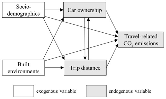
Figure 2.
The conceptual framework for the structural equation models construction.
Since the variables estimated in this paper were observed variables rather than latent variables, the SEMs without latent variables constructed in this paper can be expressed as follows [44,48]:
where y is the NY × 1 vector of endogenous variables, x is the NX × 1 vector of exogenous variables, B is the NY × NX matrix of coefficients representing the direct effects of endogenous variables on other endogenous variables, Γ is the NY × NX matrix of coefficients representing the direct effects of exogenous variables on endogenous variables, and ζ is the NY × 1 vector of errors in the equation. The ordered categorical variables in socio-demographic attributes, such as Age, Household size, Education, and Household monthly incomes per capita, were introduced directly into the models as continuous variables. The models were estimated using Amos 21.0 (IBM, Armonk, NY, USA). This paper used the Bollen-Stine bootstrap estimation method and the number of bootstraps was set to 2000, considering that the data of variables was not multivariate normal distribution [49,50].
y = By + Γx + ζ,
We revised the SEMs according to the Modification Indices (M.I.) provided by Amos 21.0. The links between the variables and the covariance between errors that can improve the model fit were added in a revised model [51]. Meanwhile, the links that were not statistically significant (p > 0.1) were removed from the models. The models were re-estimated after each modification, until the table of M.I. no longer prompted that the model needed to be modified, and the significance level of each link was above 10%.
The ratios of sample size to the number of observed variables in the SEMs constructed for commuting trips, social trips, recreational trips, and daily shopping trips are 1239/17 (≈73), 726/17 (≈43), 702/17 (≈41) and 712/17 (≈42), respectively, which are much greater than the large sample reference value (15). Therefore, the sample size can be considered to be large enough to meet the model construction and statistical requirements [52].
3. Results and Discussion
3.1. Goodness-of-Fit for SEMs
Based on the above conceptual framework, four SEM models were constructed and fitted for commuting trips, social trips, recreational trips, and daily shopping trips, respectively. All the goodness-of-fit indices for SEMs in Table 4 shows that the models fit well with the data.
Table 4.
The model fit indices for the structural equation models.
Figure 3 shows the SEM path relationship between residents’ socio-demographics, the neighborhood built environments, car ownership, trip distance, and travel-related CO2 emissions for the four purposes of the trips. Although the path relationship between the variables in these models was similar, there were still some differences: for the different purpose of trips, the factors and mechanisms that affect the travel-related CO2 emissions of residents are likely to be different, which difference needs to be measured and explored separately.
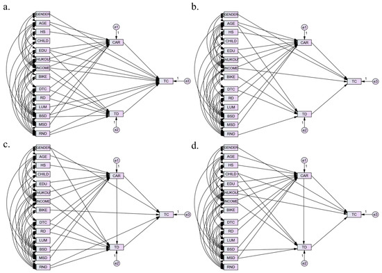
Figure 3.
The SEM path diagram for commuting trips (a), social trips (b), recreational trips (c), and daily shopping trips (d).
Table 5 shows the direct effects, indirect effects, and total effects of six neighborhood built environment variables on car ownership, trip distance, and travel-related CO2 emissions. Since the effects of socio-demographic attributes have been explored comprehensively and richly in existing studies, this paper focused on examining the direct effects and indirect effects of neighborhood built environments on the travel-related CO2 emissions of residents, aiming at providing a scientific basis for land-use planning, transport planning, residential district planning, and related policy development.
Table 5.
The standardized total, direct, and indirect effects of variables on endogenous variables.
3.2. The Interaction between Car Ownership, Trip Distance, and Travel-Related CO2 Emissions
The path diagram (Figure 3) and model results (Table 5) show that, for different purposes of trips, the relationship between car ownership and trip distance was different. For example, car ownership had an impact on trip distance for recreational and daily shopping trips but had no significant impact on trip distance for commuting and social trips. This effect of the car ownership would further indirectly affect the CO2 emissions. In general, both car ownership and trip distance have a significant positive direct effect and total effect on CO2 emissions from trips (significant level was 1%), which meant residents with cars or those traveling longer distances emit more CO2. Specifically, the effects of car ownership on travel-related CO2 emissions were the largest for commuting trips and the smallest for daily shopping trips, while the effects of trip distance on travel-related CO2 emissions were the largest for recreational trips and the smallest for commuting trips. This indicated that residents tended to use high-carbon modes for recreational trips but tended to use low-carbon modes for commuting trips, and residents with cars tended to emit more CO2 during commuting trips than during other trips. This showed that the relationship between car ownership, trip distance, and travel-related CO2 emissions would become very complex if we specifically explore them for different purposes of trips.
3.3. The Direct Effects of Neighborhood Built Environments on Travel-Related CO2 Emissions
Overall, half of the neighborhood built environment elements that we studied had no significant direct effect on CO2 emissions from commuting trips, while almost all of the elements had no significant effect on CO2 emissions from other purposes of trips. In other words, the neighborhood built environments produced more pronounced effects for commuting trips than for other purposes of trips. For commuting trips, the land-use mix, bus stop density, and road network density had a significant level of 5%, 1%, and 10% of the direct effect on travel-related CO2 emissions, respectively, while they had no significant direct effect for social and daily shopping trips. Moreover, for recreational trips, the road network density had the opposite effect. This shows that the impact of the built environment on carbon emissions for different purposes of trips is not consistent. Some built environment elements may have a direct effect for some purposes of trips but have no significant direct effect for other purposes of trips, and some may even have the opposite effect for different purposes of trips.
Specifically, the standardized coefficient of the direct effect of the land-use mix and road network density on CO2 emissions from commuting trips were −0.077 and −0.136, respectively, which meant that the more diversified the neighborhood land-use, and the denser the neighborhood road network, the less CO2 the residents emit during commuting trips. However, bus stop density had a significant direct effect on CO2 emissions from commuting trips, which indicated that providing high-density bus services did not necessarily encourage residents to choose low-carbon modes for commuting trips, especially in cities like Guangzhou, where the supply of buses is already very high. As can also be seen from Table 1, there is no obvious difference in the bus stop density of the neighborhoods located in different locations. Therefore, for the neighborhoods with an adequate supply of bus services, attempts to add more bus stops or bus lines to reduce the residents’ CO2 emissions from commuting would probably not achieve the intended effect.
Although the vast majority of built environment elements have no direct impact on CO2 emissions from other purposes of trips, it does not imply that planning intervention for the built environment is useless. If the direct effect is concerned only, the policy implications of the study are likely to be biased, because the actual impact (called the total effects) of the built environment may come from the indirect effect.
3.4. The Indirect Effects of Neighborhood Built Environments on Travel-Related CO2 Emissions
Indirect effects are a major source of the impact of neighborhood built environments on travel-related CO2 emissions, which come from intermediary variables such as car ownership and trip distance. From Table 5, we can see that the variables of distance to city public centers and metro station density had significant indirect effects on CO2 emissions from commuting trips, and for CO2 emissions from other purposes, many built environment variables also had significant indirect effects, which made them have significant total effects on CO2 emissions.
Specifically, the distance from the neighborhood to city public centers had a positive indirect effect and total effect on CO2 emissions from commuting trips at the significance of 5%, which came from influencing the mediating variables of car ownership and trip distance. This indicated that although the distance between the neighborhood and city public centers was negatively correlated with car ownership, it was positively correlated with commuting distance (with a greater standardized coefficient than car ownership) so that the distance to city public centers had a positive indirect effect and total effect on CO2 emissions from commuting trips. However, for daily shopping trips, it had a significant negative indirect effect and total effect on CO2 emissions. This implied that residents who lived far from city public centers were likely to make their daily shopping trips in the vicinity of their neighborhood with little CO2 emissions, especially for neighborhoods with well-developed commercial facilities. Although residential density had no significant direct effect on CO2 emissions for all purposes of trips, it had a significant positive indirect effect and total effect on CO2 emissions from social trips and daily shopping trips. This implied that the effect of residential density on travel-related CO2 emissions in Chinese cities is likely to be different from that in Western countries, most of which usually have a significantly negative effect [28,32]. A study on the influence factors of transportation CO2 emissions in China also demonstrated that urban population density was positively correlated with CO2 emissions from transportation [8]. Therefore, in order to promote low-carbon travel and achieve low-carbon development goals, increasing neighborhood residential density is not an effective method for Chinese cities. A similar situation also occurred with bus stop density, which had a positive indirect effect on CO2 emissions from commuting trips and recreational trips at a 10% significant level, and its total effect on them was positive (significant level was 1% for commuting trips and 10% for recreational trips). This result was inconsistent with that of many studies in Western countries. Meanwhile, for social trips and daily shopping trips, the bus stop density had a significant negative indirect effect and total effect at a 1% significant level. This indicated that although improving the neighborhood bus service supply did not necessarily encourage residents to emit less CO2 during commuting and recreational trips, it helped to reduce the CO2 emissions from social trips and daily shopping trips. Metro station density had no direct effect on CO2 emissions, but it had a significant indirect effect on them from four purposes of trips, which mainly came from the intermediary role of car ownership. Although both metro station density and bus stop density were negatively related to car ownership, the bus stop density often had a positive correlation with trip distance, for example, during commuting trips and social trips, as bus travel was likely to result in longer trip distances. Therefore, increasing the neighborhood’s subway service is more effective than increasing the bus service in promoting low-carbon travel, which is consistent with an existing study on Guangzhou [53]. Meanwhile, road network density had negative indirect and total effects on CO2 emissions from commuting, social, and recreational trips. Its indirect effects resulted from the mediating effect of trip distance, which indicated that the denser the neighborhood road network, the shorter the residents’ trip distance would be, resulting in smaller emissions of CO2. Land-use mix only had a direct effect on CO2 emissions from commuting trips but had no significant indirect effect on emissions from commuting trips and other purposes of trips.
4. Conclusions and Policy Implications
This paper used neighborhood survey data and the Travel O-D Point Intelligent Query System to calculate residents’ CO2 emissions from commuting trips, social trips, recreational trips, and daily shopping trips and measured the direct and indirect effects of neighborhood built environments on them by building structural equation models. It drew the following conclusions and planning implications: first, most of the neighborhood built environment elements had a significant total effect on CO2 emissions, which mainly came from an indirect effect through affecting the mediators, such as car ownership or trip distance, and then indirectly affecting the travel-related CO2 emissions. Therefore, it would probably underestimate the effects of neighborhood built environments on travel-related CO2 emissions and thus, mislead land-use and transport planning and its related policy development if only their direct effects were considered and their indirect effects were ignored. Second, the effects of neighborhood built environments on CO2 emissions from different purposes of trips were not consistent. Low-carbon oriented land-use and transport planning needed to fully consider the difference of the effects of the built environment on CO2 emissions for different trip purposes [54]. Third, narrowing the distance between neighborhoods and city public centers is an effective way to reduce CO2 emissions from commuting. At the same time, the commercial facilities in neighborhoods far from city public centers should also be improved, which would be beneficial for reducing the CO2 emissions from daily shopping. Meanwhile, the neighborhood’s residential density should be controlled at a livable level instead of blindly increasing its density, which has little effect on shaping the low-carbon land-use pattern. The diversification of neighborhood land-use is worth advocating. It will be helpful to reduce travel-related CO2 emissions, especially for reducing emissions from commuting trips [55,56]. For neighborhoods with a higher density of bus stops, further addition of bus stops may not effectively reduce the CO2 emissions from commuting trips and recreational trips. Instead, increasing the number of metro stations around the neighborhood and its road network density, abandoning the large blocks and wide roads, and building a good non-motorized travel environment will play a greater role in promoting residents’ low-carbon travel and travel behavior changes.
Author Contributions
W.Y. developed the main ideas of the study, gathered the data, performed the models construction and estimation, and wrote the manuscript. S.W. and X.Z. contributed to the conceptual framework of this paper, played an important role in interpreting of the results and participated in revising the manuscript and proofreading the article. All authors read and approved the final manuscript.
Acknowledgments
This work was supported by the National Natural Science Foundation of China (41701169, 41601151), the Philosophy and Social Sciences Planning Project of Guangdong Province (GD17YSH01), the Natural Science Foundation of Guangdong Province (2016A030310149) and the Pearl River S&T Nova Program of Guangzhou.
Conflicts of Interest
The authors declare no conflict of interest.
References
- IEA (International Energy Agency). CO2 Emissions from Fuel Combustion; IEA: Paris, France, 2016. [Google Scholar]
- Fuglestvedt, J.; Berntsen, T.; Myhre, G.; Rypdal, K.; Skeie, R.B. Climate forcing from the transport sectors. Proc. Natl. Acad. Sci. USA 2008, 105, 454–458. [Google Scholar] [CrossRef] [PubMed]
- Marsden, G.; Rye, T. The governance of transport and climate change. J. Transp. Geogr. 2010, 18, 669–678. [Google Scholar] [CrossRef]
- Brand, C.; Tran, M.; Anable, J. The UK transport carbon model: An integrated life cycle approach to explore low carbon futures. Energy Policy 2012, 41, 107–124. [Google Scholar] [CrossRef]
- IEA (International Energy Agency). CO2 Emissions from Fuel Combustion Highlights 2010; IEA: Paris, France, 2010. [Google Scholar]
- Zhao, P.; Lü, B.; Roo, G.D. Impact of the jobs-housing balance on urban commuting in Beijing in the transformation era. J. Transp. Geogr. 2011, 19, 59–69. [Google Scholar] [CrossRef]
- Zhao, P. Sustainable urban expansion and transportation in a growing megacity: Consequences of urban sprawl for mobility on the urban fringe of Beijing. Habit. Int. 2010, 34, 236–243. [Google Scholar] [CrossRef]
- Yang, W.; Li, T.; Cao, X. Examining the impacts of socio-economic factors, urban form and transportation development on CO2 emissions from transportation in china: A panel data analysis of China’s provinces. Habit. Int. 2015, 49, 212–220. [Google Scholar] [CrossRef]
- Handy, S.L.; Krizek, K.J. The role of travel behavior research in reducing the carbon footprint: From the US perspective. In Proceedings of the Triennial Meeting of the International Association of Travel Behavior Research, Jaipur, India, 13–18 December 2009. [Google Scholar]
- Crane, R. The influence of urban form on travel: An interpretive review. J. Plan. Lit. 2000, 15, 3–23. [Google Scholar] [CrossRef]
- Handy, S.L.; Boarnet, M.G.; Ewing, R.; Killingsworth, R.E. How the built environment affects physical activity: Views from urban planning. Am. J. Prev. Med. 2002, 23, 64–73. [Google Scholar] [CrossRef]
- Handy, S.; Cao, X.; Mokhtarian, P. Correlation or causality between the built environment and travel behavior? Evidence from Northern California. Transp. Res. Part D Transp. Environ. 2005, 10, 427–444. [Google Scholar] [CrossRef]
- Boarnet, M.G. A broader context for land use and travel behavior, and a research agenda. J. Am. Plan. Assoc. 2011, 77, 197–213. [Google Scholar] [CrossRef]
- Ewing, R.; Cervero, R. Travel and the built environment. J. Am. Plan. Assoc. 2010, 76, 265–294. [Google Scholar] [CrossRef]
- Ewing, R.; Cervero, R. Travel and the built environment: A synthesis. Transp. Res. Record J. Transp. Res. Board 2001, 1780, 87–114. [Google Scholar] [CrossRef]
- Cao, X.J. Land use and transportation in China. Transp. Res. Part D Transp. Environ. 2017, 52 Pt B, 423–427. [Google Scholar] [CrossRef]
- Cao, X.; Yang, W. Examining the effects of the built environment and residential self-selection on commuting trips and the related CO2 emissions: An empirical study in Guangzhou, China. Transp. Res. Part D Transp. Environ. 2017, 52 Pt B, 480–494. [Google Scholar] [CrossRef]
- Lakshmanan, T.R.; Han, X. Factors underlying transportation CO2 emissions in the USA: A decomposition analysis. Transp. Res. Part D Transp. Environ. 1997, 2, 1–15. [Google Scholar] [CrossRef]
- Timilsina, G.R.; Shrestha, A. Transport sector CO2 emissions growth in Asia: Underlying factors and policy options. Energy Policy 2009, 37, 4523–4539. [Google Scholar] [CrossRef]
- Wang, W.W.; Zhang, M.; Zhou, M. Using LMDI method to analyze transport sector CO2 emissions in China. Energy 2011, 36, 5909–5915. [Google Scholar] [CrossRef]
- Lu, I.J.; Lin, S.J.; Lewis, C. Decomposition and decoupling effects of carbon dioxide emission from highway transportation in Taiwan, Germany, Japan and South Korea. Energy Policy 2007, 35, 3226–3235. [Google Scholar] [CrossRef]
- Bueno, G. Analysis of scenarios for the reduction of energy consumption and GHG emissions in transport in the Basque country. Renew. Sustain. Energy Rev. 2012, 16, 1988–1998. [Google Scholar] [CrossRef]
- He, D.; Liu, H.; He, K.; Meng, F.; Jiang, Y.; Wang, M.; Zhou, J.; Calthorpe, P.; Guo, J.; Yao, Z. Energy use of, and CO2 emissions from China’s urban passenger transportation sector: Carbon mitigation scenarios upon the transportation mode choices. Transp. Res. Part A Policy Pract. 2013, 53, 53–67. [Google Scholar] [CrossRef]
- Matsuhashi, K.; Ariga, T. Estimation of passenger car CO2 emissions with urban population density scenarios for low carbon transportation in Japan. IATSS Res. 2016, 39, 117–120. [Google Scholar] [CrossRef]
- Zhou, G.; Chung, W.; Zhang, X. A study of carbon dioxide emissions performance of China’s transport sector. Energy 2013, 50, 302–314. [Google Scholar] [CrossRef]
- Cui, Q.; Li, Y. An empirical study on the influencing factors of transportation carbon efficiency: Evidences from fifteen countries. Appl. Energy 2015, 141, 209–217. [Google Scholar] [CrossRef]
- Lin, W.; Chen, B.; Xie, L.; Pan, H. Estimating energy consumption of transport modes in China using DEA. Sustainability 2015, 7, 4225–4239. [Google Scholar] [CrossRef]
- Barla, P.; Miranda-Moreno, L.F.; Lee-Gosselin, M. Urban travel CO2 emissions and land use: A case study for Quebec City. Transp. Res. Part D-Transp. Environ. 2011, 16, 423–428. [Google Scholar] [CrossRef]
- Ko, J.; Park, D.; Lim, H.; Hwang, I.C. Who produces the most CO2 emissions for trips in the Seoul metropolis area? Transp. Res. Part D Transp. Environ. 2011, 16, 358–364. [Google Scholar] [CrossRef]
- Brand, C.; Goodman, A.; Rutter, H.; Song, Y.; Ogilvie, D. Associations of individual, household and environmental characteristics with carbon dioxide emissions from motorised passenger travel. Appl. Energy 2013, 104, 158–169. [Google Scholar] [CrossRef] [PubMed]
- Brand, C. “Hockey sticks” made of carbon unequal distribution of greenhouse gas emissions from personal travel in the United Kingdom. Transp. Res. Rec. 2009, 2139, 88–96. [Google Scholar] [CrossRef]
- Zahabi, S.A.H.; Miranda-Moreno, L.; Patterson, Z.; Barla, P.; Harding, C. Transportation greenhouse gas emissions and its relationship with urban form, transit accessibility and emerging green technologies: A Montreal case study. Procedia Soc. Behav. Sci. 2012, 54, 966–978. [Google Scholar] [CrossRef]
- Hong, J.; Goodchild, A. Land use policies and transport emissions: Modeling the impact of trip speed, vehicle characteristics and residential location. Transp. Res. Part D Transp. Environ. 2014, 26, 47–51. [Google Scholar] [CrossRef]
- Hong, J. Non-linear influences of the built environment on transportation emissions: Focusing on densities. J. Transp. Land Use 2015, 10, 229–240. [Google Scholar] [CrossRef]
- Ma, J.; Liu, Z.; Chai, Y. The impact of urban form on CO2 emission from work and non-work trips: The case of Beijing, China. Habit. Int. 2015, 47, 1–10. [Google Scholar] [CrossRef]
- Liu, Z.; Ma, J.; Chai, Y. Neighborhood-scale urban form, travel behavior, and CO2 emissions in Beijing: Implications for low-carbon urban planning. Urban Geogr. 2017, 38, 381–400. [Google Scholar] [CrossRef]
- Frank, L.D.; Andresen, M.A.; Schmid, T.L. Obesity relationships with community design, physical activity, and time spent in cars. Am. J. Prev. Med. 2004, 27, 87–96. [Google Scholar] [CrossRef] [PubMed]
- Moniruzzaman, M.; Páez, A.; Habib, K.M.N.; Morency, C. Mode use and trip length of seniors in montreal. J. Transp. Geogr. 2013, 30, 89–99. [Google Scholar] [CrossRef]
- Aguiléra, A.; Voisin, M. Urban form, commuting patterns and CO2 emissions: What differences between the municipality’s residents and its jobs? Transp. Res. Part A Policy Pract. 2014, 69, 243–251. [Google Scholar] [CrossRef]
- Wang, Y.; Yang, L.; Han, S.; Li, C.; Ramachandra, T.V. Urban CO2 emissions in Xi’an and Bangalore by commuters: Implications for controlling urban transportation carbon dioxide emissions in developing countries. Mitig. Adapt. Strateg. Glob. Chang. 2017, 22, 993–1019. [Google Scholar] [CrossRef]
- Entwicklungsbank, K. Transport in China: Energy Consumption and Emissions of Different Transport Modes; Institute for Energy and Environmental Research Heidelberg: Heidelberg, Germany, 2008. [Google Scholar]
- Bagley, M.N.; Mokhtarian, P.L. The impact of residential neighborhood type on travel behavior: A structural equations modeling approach. Ann. Reg. Sci. 2002, 36, 279–297. [Google Scholar] [CrossRef]
- Van Acker, V.; Witlox, F. Car ownership as a mediating variable in car travel behaviour research using a structural equation modelling approach to identify its dual relationship. J. Transp. Geogr. 2010, 18, 65–74. [Google Scholar] [CrossRef]
- Cao, X.; Mokhtarian, P.L.; Handy, S.L. Do changes in neighborhood characteristics lead to changes in travel behavior? A structural equations modeling approach. Transportation 2007, 34, 535–556. [Google Scholar] [CrossRef]
- Cervero, R.; Murakami, J. Effects of built environments on vehicle miles traveled: Evidence from 370 US urbanized areas. Environ. Plan. A 2010, 42, 400–418. [Google Scholar] [CrossRef]
- Aditjandra, P.T.; Cao, X.J.; Mulley, C. Understanding neighbourhood design impact on travel behaviour: An application of structural equations model to a British metropolitan data. Transp. Res. Part A Policy Pract. 2012, 46, 22–32. [Google Scholar] [CrossRef]
- Shen, Q.; Chen, P.; Pan, H. Factors affecting car ownership and mode choice in rail transit-supported suburbs of a large Chinese city. Transp. Res. Part A Policy Pract. 2016, 94, 31–44. [Google Scholar] [CrossRef]
- Lu, X.; Pas, E.I. Socio-demographics, activity participation and travel behavior. Transp. Res. Part A Policy Pract. 1999, 33, 1–18. [Google Scholar] [CrossRef]
- Chowdhury, S.; Ceder, A. A psychological investigation on public-transport users’ intention to use routes with transfers. Int. J. Transp. 2013, 1, 1–20. [Google Scholar] [CrossRef]
- Ma, L.; Dill, J.; Mohr, C. The objective versus the perceived environment: What matters for bicycling? Transportation 2014, 41, 1135–1152. [Google Scholar] [CrossRef]
- Wu, M. Structural Equation Modeling: The Operation and Application of AMOS; Chongqing University Press: Chongqing, China, 2010. (in Chinese) [Google Scholar]
- Stevens, J.P. Applied Multivariate Statistics for the Social Sciences; Routledge: Abingdon, UK, 2012. [Google Scholar]
- Yang, W.; Chen, B.Y.; Cao, X.; Li, T.; Li, P. The spatial characteristics and influencing factors of modal accessibility gaps: A case study for Guangzhou, china. J. Transp. Geogr. 2017, 60, 21–32. [Google Scholar] [CrossRef]
- Wang, S.; Liu, P. China’s city-level energy-related CO2 emissions: Spatio-temporal patterns and driving forces. Appl. Energy 2017, 200, 204–214. [Google Scholar] [CrossRef]
- Wang, S.; Liu, X.; Zhou, C.; Hu, J.; Ou, J. Examining the impacts of socioeconomic factors, urban form, and transportation networks on CO2 emissions in China’s megacities. Appl. Energy 2017, 185, 189–200. [Google Scholar] [CrossRef]
- Wang, S.; Fang, C.; Wang, Y.; Huang, Y.; Ma, H. Quantifying the relationship between urban development intensity and carbon dioxide emissions using a panel data analysis. Ecol Indicators 2015, 49, 121–131. [Google Scholar] [CrossRef]
© 2018 by the authors. Licensee MDPI, Basel, Switzerland. This article is an open access article distributed under the terms and conditions of the Creative Commons Attribution (CC BY) license (http://creativecommons.org/licenses/by/4.0/).