Vehicle Trajectory Prediction Based on Local Dynamic Graph Spatiotemporal–Long Short-Term Memory Model

Abstract

Traffic congestion and frequent traffic accidents have become the main problems affecting urban traffic. The effective location prediction of vehicle trajectory can help alleviate traffic congestion, reduce the occurrence of traffic accidents, and optimize the urban traffic system. Vehicle trajectory is closely related to the surrounding Point of Interest (POI). POI can be considered as the spatial feature and can be fused with trajectory points to improve prediction accuracy. A Local Dynamic Graph Spatiotemporal–Long Short-Term Memory (LDGST-LSTM) was proposed in this paper to extract and fuse the POI knowledge and realize next location prediction. POI semantic information was learned by constructing the traffic knowledge graph, and spatial and temporal features were extracted by combining the Graph Attention Network (GAT) and temporal attention mechanism. The effectiveness of LDGST-LSTM was verified on two datasets, including Chengdu taxi trajectory data in August 2014 and October 2018. The accuracy and robustness of the proposed model were significantly improved compared with the benchmark models. The effects of major components in the proposed model were also evaluated through an ablation experiment. Moreover, the weights of POI that influence location prediction were visualized to improve the interpretability of the proposed model.

1. Introduction

Traffic congestion and frequent traffic accidents have become serious problems affecting urban traffic with the rapid development of cities [1]. The Intelligent Transportation System (ITS) has been proposed to alleviate these traffic problems. The location prediction of vehicle trajectory is one of the research topics relating to the ITS [2]. Through effective location prediction, traffic congestion can be alleviated, which is of great significance in terms of optimizing traffic management. The goal of vehicle location prediction is to predict the next location of the vehicle according to the observed trajectory data [3]. Deep learning methods have been widely used in vehicle trajectory location prediction. Vehicle trajectory is usually considered a time series since it is a sequence of sampled points [1]. Long Short-Term Memory (LSTM) was mainly used to deal with time sequences. Convolution Neural Network (CNN) was used by Guo [1] to extract the spatial features of vehicles, and a Deep Bidirectional Long Short-Term Memory (DBLSTM) model was used to extract the temporal features to realize the location prediction of vehicles. A LSTM was applied by Li et al. [4] to capture the temporal features between vehicles and design a convolutional social pooling network to capture spatial features to predict vehicle trajectory. A weighted support vector regression algorithm was proposed by Liao [5] to allocate weight according to the calculation and comparison of trajectory points to achieve vehicle location prediction, improving the accuracy and robustness of the results. Methods based on deep learning algorithms can effectively improve prediction accuracy and reduce error. Through feature mining and extraction, deep learning models can effectively improve the accuracy and robustness of the prediction results. However, complex road structures and the surrounding environment could become the factors affecting vehicle location prediction. The impact of surrounding buildings, or to say, Point of Interest (POI), on prediction under complex traffic environments was usually ignored in the existing research. Based on this situation, the performance of vehicle location prediction in the real traffic network cannot be satisfied. Therefore, how to integrate external features with vehicle trajectory to improve the accuracy and robustness of the model needs further research.

Knowledge graph (KG), Graph Attention Network (GAT), and time attention mechanism are popular methods used lately in the field of transportation and have shown better performance in improving the accuracy and robustness of the model [6]. The knowledge graph can help fuse features. GAT can be used as a spatial attention mechanism to effectively extract spatial features, and a temporal attention mechanism can effectively extract temporal features. The application of knowledge graph has developed rapidly in the field of transportation. For example, a multi-layer traffic knowledge graph model was proposed by Wang [7] to realize destination prediction by modeling the complex traffic network, weighted summing, and fusing different node features. The driving intention in the traffic network is affected by the functional area and the surrounding Point of Interest (POI) [8]. Therefore, it is important to predict the location of vehicle trajectory by designing a traffic knowledge graph. The accuracy can be improved by interacting the vehicle trajectory with the surrounding environments [8]. Point of interest (POI) generally refers to a location or a specific point on a map or in a geographical area. Those points are often marked on maps to help people navigate and discover places of interest, such as hotels, restaurants, shopping malls, or other noteworthy locations. In trajectory prediction, the driving intention of vehicles is closely related to the surrounding POI [8]. Therefore, POI can be considered as prior knowledge and spatial feature to help model understanding of the context. It can be fused with trajectory points to improve prediction accuracy [9]. The trajectory may change when there are traffic jams or traffic accidents, and the POI knowledge around trajectory points has an impact on the future trend. It is of significance to the optimization of traffic management by integrating POI knowledge and vehicle trajectory to realize position prediction and improve the accuracy of the prediction. Graph Attention Network (GAT) [10] and various temporal attention mechanisms [11] are also widely used for extracting spatial and temporal features. A new GAT is proposed by Su et al. [12] to allocate attention to explain and express the spatial correlation of road networks, as well as effectively capture the dynamic update of the adjacent transformation matrix. LSTM combined with the attention mechanism was proposed by Ali et al. [13] to capture temporal features. However, how to fuse the surrounding environment features such as POI and the synergy of knowledge graph, GAT, and temporal attention mechanism on location prediction tasks still lacks research.

A Local Dynamic Graph Spatiotemporal–Long Short-Term Memory (LDGST–LSTM) is proposed in this paper to predict the next location of vehicle trajectory. Through the proposed model, POI knowledge is extracted and fused by constructing a traffic knowledge graph. Additionally, GAT and temporal attention mechanisms are combined to improve the accuracy, robustness, and interpretability of the prediction. The main contributions of this paper are as follows.

• Knowledge graph and spatiotemporal attention mechanisms were combined in this paper to predict the vehicle location at the next moment. POI was integrated with historical trajectory, and the POI weights that affect the prediction were visualized additionally. Regions that have a great impact on the prediction are explored, and the interpretability of the model was enhanced.
• A global traffic knowledge graph was constructed to learn and represent POI semantic information. POI nodes were considered as the entity, and the connection between POI was considered as the relationship. The representation vector of each node was obtained by using the Translate Embedding (TransE) algorithm and was considered as the feature vector for vehicle location prediction.
• A spatiotemporal attention mechanism was designed to allocate weights for spatial and temporal features, thus enhancing the interpretability and accuracy of the model. The weight distribution of spatial features was achieved through GAT to obtain the corresponding graph representation vector. LSTM combined with a multi-head attention mechanism was applied to allocate weights of trajectory points at different time steps to improve the prediction accuracy.

Section 2 introduces a thorough review of the research on vehicle trajectory prediction from three aspects: deep learning, knowledge graphs, and attention mechanisms. The basic concepts and studied problems are formally defined in Section 3. The research methodology and details of the LDGST-LSTM model are presented in Section 4. Then, Section 5 provides a description of the experiment settings. Experiments on robustness, accuracy, and ablation are conducted to confirm the effectiveness of the proposed model. In Section 6, the findings of this paper are outlined. Moreover, limitations and further directions are also described.

2. Related Work

This section will provide a literature review on related works, including vehicle location prediction, knowledge graph, and attention mechanism.

2.1. Vehicle Trajectory Location Prediction

The deep learning method is widely used in location prediction of vehicle trajectory. A vehicle trajectory prediction model combining deep encoder–decoder and neural network was designed by Fan et al. [14]. Multiple segments were processed and corrected by using the deep neural network model, which improved the accuracy of the prediction and alleviated long-term dependences [15]. Kalatian and Farooq [16] proposed a new multi-input LSTM to fuse sequence data with context information of the environment. It can reduce prediction error, but more external features that could improve the prediction performance are ignored. Graph Convolutional Network (GCN) combined with its variant model were proposed by An et al. [17] to realize vehicle trajectory prediction in urban traffic systems. Through this conjunction, the model can effectively capture spatiotemporal features, therefore improving the effectiveness of the prediction.

Methods based on deep learning algorithms can effectively improve prediction accuracy and reduce error. Through feature mining and extraction, a deep learning model can effectively improve its accuracy and robustness. Methods based on statistical methods are also widely used in traffic prediction because of their interpretability. The statistical model was used to calculate the possible transition probability, which can help understand and explain mobile individual behaviors. By utilizing sensor data and modeling techniques, Zambrano-Martinez et al. [18] applied statistical methods such as regression and clustering to analyze the trajectory data, which provided insights into the complex dynamics of urban traffic. Zhang et al. [19] introduced an innovative method incorporating fuzzy logic and genetic algorithms for short-term traffic congestion prediction. However, the impact of surrounding buildings, such as Point of Interest (POI), on prediction under complex traffic environments is usually ignored in the existing research. Therefore, how to better integrate external factors such as POI features needs further research to help improve prediction performance.

The efficiency and accuracy of vehicle location prediction can be enhanced by combining vehicle trajectory with road networks in data preprocessing. For example, original vehicle trajectory points were replaced with marked nodes or roads of road networks by Fan [14] to realize location prediction. However, only the location information was considered in the proposed method, and external factors such as driving intentions or preferences that have significant impacts on prediction results were ignored.

2.2. Knowledge Graph

Knowledge graph is one of the most popular representation methods, which describes entities and their relationships in a structured triple. Each triple is composed of a head entity, a tail entity, and their relationship. The knowledge graph can be combined with deep learning models to learn the representation of the entities and relationships to realize prediction tasks. It can make contributions in the fields of medical treatment, national defense, transportation, and network information security [20,21].

A knowledge graph can be seen as a structured representation of contextual information on the map. It helps the model understand relationships between different elements in the environment, such as the proximity of points of interest (POIs), road structures, or historical traffic patterns. The knowledge graph enriches the model’s understanding of the environment, allowing it to make predictions with a deeper awareness of the spatial context. Additionally, the model should be adaptive to evolving conditions like construction zones or changes in traffic patterns.

Translating Embedding (TransE) is one of the typical models of knowledge graph [22]. A TransGraph model based on TransE was proposed by Chen et al. [23] to learn the structural features. Moreover, the knowledge graph is also widely used in machine learning. An open-source tool, DGL-KE, which can be effectively used to calculate the embedded representation of the knowledge graph, was proposed by Zheng et al. [24] to execute the TransE algorithm. This tool can speed up the training of entities and relationships in the knowledge graph through multi-processing, multi-GPU, and distributed parallelism. A traffic mode knowledge graph framework based on historical traffic data was proposed by Ji and Jin [25] to capture the traffic status and congestion propagation mode of road segments. This framework had pioneering significance for the knowledge graph in the prediction of traffic congestion propagation. Wang et al. [26] proposed a method of embedding the temporal knowledge graph through a sparse transfer matrix. Static and temporal dynamic knowledge graphs were employed to capture global and local embedding knowledge, respectively. This approach helped alleviate issues related to inconsistent parameter scalability when learning embeddings from different datasets.

More semantic knowledge can be considered in the knowledge graph to enhance the interpretability of complex models [21]. In addition, how to learn entities and relationships with low frequency better, how to integrate context into graph embedding learning better, and how to combine the graph embedding algorithm with other algorithms are future research directions.

2.3. Attention Mechanism

Graph Attention Network (GAT) is widely used in the field of transportation to obtain the spatial correlation between nodes. Wang et al. [27] proposed a trend GAT model to predict traffic flow. The transmission among comparable nodes was facilitated by constructing a spatial graph structure, effectively addressing the issue of spatial heterogeneity. A spatiotemporal multi-head GAT model was proposed by Wang and Wang [28] to realize traffic prediction. Spatial features were captured through a multi-head attention mechanism, and temporal features were captured through a full-volume transformation linear gated unit. The spatiotemporal correlation between traffic flow and traffic network was integrated to reduce the prediction error. Wang et al. [29] proposed a dynamic GAT model to realize traffic prediction. The spatial feature was extracted through the use of a node embedding algorithm based on the dynamic attention mechanism, and the temporal feature was extracted through the use of a gated temporal CNN in this model.

The temporal attention mechanism is also widely applied in traffic research. The temporal attention mechanism can enhance the understanding of the time correlation among research objectives. A temporal attention perception dual GCN was proposed by Cai et al. [30] to realize air traffic prediction. The historical flight and time evolution pattern were characterized through a temporal attention mechanism. Yan et al. [31] designed a gated self-attention mechanism module to realize the interaction between the current memory state and the long-term relationship. Chen et al. [32] applied a multi-head attention mechanism to mine the features of fine-grained spatiotemporal dynamics. A one-dimensional convolution LSTM model based on the attention mechanism was proposed by Wang et al. [33] to realize traffic prediction. Through the attention mechanism, diverse features from multiple sources were integrated.

Spatial attention can make the model focus on the important areas of a scene, and temporal attention is about understanding the sequence of trajectory points. By paying more attention to significant spatial and temporal features, the model can dynamically adjust its focus, prioritizing crucial information based on its significance in both space and time. The spatiotemporal attention mechanism can obtain reasonable weights of the features under complex traffic environments, therefore improving the interpretability of the model. GAT can be considered as a spatial attention mechanism to capture spatial features, and the multi-head attention mechanism can be considered to be a temporal attention mechanism to capture temporal features. Therefore, it is meaningful and important to combine GAT and temporal attention mechanisms when realizing vehicle trajectory location prediction.

Spatial and temporal attention mechanisms enable the model to dynamically adjust its focus, making it more resilient to changes and uncertainties in the environment. Navigating through intricate urban environments necessitates comprehending not just the immediate surroundings but also the broader context. The combination of knowledge graph and attention mechanisms allows the model to capture complex relationships, making it more effective in handling intricate scenarios where standard models might struggle. By incorporating these components, these approaches can create a more context-aware trajectory prediction model capable of adapting to diverse and dynamic real-world scenarios.

3. Problem Statement

In this section, some basic concepts and notations in this paper are first introduced, and then the studied problem is formally defined.

Definition 1

(Raw trajectory $T_i$). A raw vehicle trajectory is usually represented by a sequence of points continuously sampled by the Global Positioning System (GPS). Given a raw trajectory dataset $Traj=\{T_1,T_2,\dots T_n\}$, the trajectory $i$, $T_i=\left\{P_{i1,}{P}_{i2},\dots ,P_{ik}\right\}$, is defined as a sequence of sampled points $P_{ij}$, where $P_{ij}\in {\mathbb{R}}^2$, $i\in \left(\mathrm{1,2},\dots ,n\right),j\in \left(\mathrm{1,2},\dots ,k\right)$. A sampled point $P_{ij}$ is defined as a tuple $({lng}_{ij},{lat}_{ij})$ which represents the longitude and latitude of the GPS point at timestamp $j$. Due to varying sampling rate, trajectory data may have irregular distribution characteristics. For example, the data may be dense in some areas of the map but sparse in other areas.

Definition 2

(Point of Interest $Q_u$). Point Of Interest (POI) can be denoted as a spatial representation of urban infrastructure such as schools, hospitals, restaurants and so on. It can reflect land use and urban functional characteristics and has potential semantic information. Its distribution influences the intentions of travel. POI can be classified into different types. Given a POI dataset with $h$ types $POI=\{Q_1,Q_2,\dots ,Q_h\}$, the type $u$ of POI $Q_u=\{I_{u1},I_{u2},\dots I_{um}\}$ is defined as a set of points $I_{uj}$, where $u\in \left(1,\dots ,h\right), j\in \left(1,\dots ,m\right)$. A POI $I_{uj}=({name}_{uj}, {address}_{uj},{lng}_{uj},{lat}_{uj},{attribute}_{uj})$ is a five-tuple, that represents the semantic information including the name, address, longitude, latitude, as well as the attribute of the $j^{th}$ POI. In this paper, eleven different categories of POI are applied, including stores, entertainment, food, hotels, scenic spots, finance, government, company, hospitals, life services, and sports.

Definition 3

(Road network $G$). A road network is defined as a graph $G=(V,E,A)$, where $V$ is the set of nodes; each $v_i$ denotes a road segment. $E$ is the set of edges connecting nodes, and each $e_{i,j}=(v_i,v_j)$ denotes the connectivity between road segment $v_i$ and $v_j$. The adjacency matrix of the graph can be denoted as $A\in {\mathbb{R}}^{\left|V\right|\times \left|V\right|}$, and semantic information of different POI categories are considered as features. Each element $a_{i,j}$ in this matrix is a binary value, which is 1 when road segment $v_i$ is adjacent to $v_j$ and 0 otherwise.

Definition 4

(Normalized trajectory $N{T}_i$). Raw trajectory $T_i$ will be processed through a data conversion layer in this paper and transformed into a trajectory in normalization form $N{T}_i$. Due to the measurement error, it is not appropriate to directly input raw trajectory to the model. Given a raw trajectory dataset $Traj=\{T_1,T_2,\dots T_n\}$, the trajectory $T_i=\left\{P_{i1,}{P}_{i2},\dots ,P_{ik}\right\}$. Match each point $P_{ij}$ to the nearest node of the road network. A normalized point $N{P}_{ij}$ is defined as a tuple $(v{lng}_{ij},v{lat}_{ij})$, which represents the longitude and latitude of node $j$. A normalized trajectory $N{T}_i$ is then defined as a sequence of road segments after projection.

Definition 5

(Normalized POI $N{Q}_u$). Match each POI $I_{uj}$ to the nodes of road network that has the shortest projection distance. A normalized POI $N{I}_{uj}$ is defined as the corresponding road segment after projection, and POI semantic information is assigned to the matched nodes as node features. The normalized POI of type $u$ is denoted as $N{Q}_u$ and the semantic information of the normalized POI $j$ of type $u$ is denoted as ${NI}_{uj}$.

Definition 6

(POI Knowledge graph ${KG}^{POI}$). Defining a knowledge graph ${KG}^{POI}=(E^{POI},R^{POI},T^{POI})$, where $E^{POI}=\{e_1,e_2,e_3,\dots e_m\}$ is the POI entity set, and where $m$ is the number of the POI entities. $R^{POI}=\{r_1,r_2,r_3,\dots r_n\}$ is the POI relationship set, where $n$ is the number of the POI relationship. $T^{POI}=\{(h_{POI},l_{POI},t_{POI})\}$ is a triple set, which refers to head entity, relation, and tail entity, respectively.

Problem 

(Vehicle trajectory location prediction). Given a raw trajectory dataset $Traj=\{T_1,T_2,\dots T_n\}$ and a road network $G$, for current point $P_{ij}$ of the trajectory $T_i$, the task aims to predict the next location $P_{ij+1}$, which is a tuple $({lng}_{ij+1},{lat}_{ij+1})$ consisting of the longitude and latitude of a GPS point at timestamp $j+1$.

4. Methodology

Vehicle trajectory is a sequence of continuously sampled points, and its intention is closely related to the Point of Interest (POI). The semantic information of POI near each trajectory point may have an impact on the next location prediction. Therefore, a Local Dynamic Graph Spatiotemporal–Long Short-Term Memory model (LDGST-LSTM) was proposed in this paper to realize location prediction for vehicle trajectory and explore the impact weight of the nearby POI.

Raw vehicle trajectory and POI were first matched to the traffic network through the data conversion layer in the proposed model. The data of POI and road network were extracted from an open-source map website, OpenStreetMap (OSM). Then, a global POI Knowledge Graph (KG) was constructed to obtain the representation vectors of the POI entities in the global POI knowledge extraction layer. Based on the global knowledge graph, local graphs related to each trajectory point were generated, and the graph representation vector was captured through the Graph Attention Network (GAT) in the local dynamic graph generation module. Finally, trajectory points with the related graph representation vectors were input into the Long Short-Term Memory model (LSTM) with a multi-head temporal attention mechanism (T-Attn) in the trajectory prediction layer to predict the next location.

In this section, details of the proposed model LDGST-LSTM are provided, which consists of four major components, as follows: a data conversion layer, a global POI knowledge extraction layer, a local dynamic graph generation module, and a trajectory prediction layer. The overall framework is first described in Section 4.1. Then, each component in this model is specifically introduced in Section 4.2, Section 4.3, Section 4.4, Section 4.5.

4.1. Overall Framework

The overall framework of LDGST-LSTM is shown in Figure 1. There are four major components in the proposed model: (1) a data conversion layer, (2) a global POI knowledge extraction layer, (3) a local dynamic generation module, and (4) a trajectory prediction layer. Additionally, the local dynamic generation module is concluded in the trajectory prediction layer. The observed vehicle trajectory $T_i=\{P_{ij-t},P_{ij-t+1},\dots ,P_{ij}\}$ was considered as the input of the model, and the predicted next location $P_{ij+1}$ of the trajectory at timestamp $j+1$ was considered the output.

Figure 1. The overall framework of Local Dynamic Graph Spatiotemporal–Long Short-Term Memory (LDGST-LSTM) with four main components, as follows: (1) data conversion layer, (2) global POI knowledge extraction layer, (3) local dynamic generation module, and (4) trajectory prediction layer.

As shown in Figure 1, vehicle trajectory $T_i$ was the input of the model. Firstly, normalized trajectory $N{T}_i$ and normalized POI $N{Q}_u$ were obtained through map matching and proximity algorithm, respectively, in the data conversion layer. Then, the representation vector ${V^{POI}}_{ij}$ of every POI was trained through the usage of the Translating Embedding (TransE) algorithm based on the knowledge graph in the global POI knowledge extraction layer. It will be considered semantic features of the trajectory points. In the trajectory prediction layer, local graphs ${G^{\prime }}_{ij-t:j}$ related to trajectory points $P_{ij-t:j}$ were first generated, and the corresponding graph representation vectors ${NRV}_{ij-t:j}$ were obtained through GAT in the local dynamic graph generation module. Normalized trajectory points $N{P}_{ij-t:j}$ and corresponding graph representation vectors $NP{V}_{ij-t:j}$ were then concatenated and input into LSTM with a multi-head attention mechanism. The model finally output the predicted next location $P_{ij+1}$ of the trajectory. The overall framework can be denoted through the use of the following Formulas (1)–(4), where $P_{j-t:j}=(P_{j-t},P_{j-t+1},\dots ,P_j)$.

• Data conversion layer:

$$T_i\stackrel{map matching}{\to }{NT}_i,Q_u\stackrel{proximity alg.}{\to }N{Q}_u$$

(1)

• Global POI knowledge extraction layer:

$$\left[{KG}^{POI},N{Q}_u\right]\stackrel{TransE}{\to }{V^{POI}}_{ij}$$

(2)

• Local dynamic graph generation module:

$$P_{ij-t:j}\stackrel{{V^{POI}}_{ij}}{\to }{G^{\prime }}_{ij-t:j}\stackrel{GAT}{\to }{NRV}_{ij-t:j}$$

(3)

• Trajectory prediction layer:

$${NP}_{ij-t:j}{;NRV}_{ij-t:j}{\stackrel{LSTM}{\to }P}_{ij+1}$$

(4)

4.2. Data Conversion Layer

This section will introduce road network data, trajectory data conversion and POI data conversion specifically.

4.2.1. Road Network

The open-source map website Open Street Map (OSM) provided the urban road network data needed in this work. Taking Chengdu as an example, the road network is shown in Figure 2 and it contains three parts of information. Figure 2a represents the road vector map and Figure 2b is the node vector map. Figure 2c visualizes the partial satellite projection map of Chengdu along with the node vectors of road (the red dots). This paper only maintains the road network data within the Third Ring Road of Chengdu as the research area, which can mainly represent the urban district.

Figure 2. Road network of Chengdu: (a) road vector map; (b) node vector map; (c) satellite projection map.

4.2.2. Trajectory Data Conversion

In the data conversion layer, raw trajectory data were converted into a normalized trajectory. Every point was denoted by the latitude and longitude corresponding to the matched road network node. The original geographic coordinate system (GCJ-02) of the trajectory data was first converted to WGS84, the geographic coordinate system of the road network data in this paper. A predetermined threshold was taken into consideration as the radius to search for candidate points, and the candidate points with the shortest distance were chosen as the normalized trajectory points. This approach was based on the earlier map-matching work of Lou et al. [34]. Points that were not successfully matched will be deleted.

4.2.3. POI Data Conversion

POI data of Chengdu in 2018 were used in this paper. The proximity algorithm was used in ArcGIS, and the nearest nodes were selected in the road network for each POI point based on distance. The context information of POI points was matched to the relevant nodes as the normalized POIs. POIs of different types were matched to the nodes of the road network. Taking life services (black dots), food (orange dots), and hospitals (blue dots) as examples, the partially matched visualization of POI can be seen in Figure 3.

Figure 3. Partial visualization of normalized POI.

4.3. Global POI Knowledge Extraction Layer

A global graph $G=(V,E,A)$ and a knowledge graph ${KG}^{POI}=(E^{POI},R^{POI},T^{POI})$ were constructed in the global POI knowledge extraction layer, as shown in Figure 4. The entity set, relationship set, and related triples were defined to study the representation vectors of each POI entity through TransE algorithm. In the defined global graph, each node in the global graph contained the related POI knowledge through the data conversion layer.

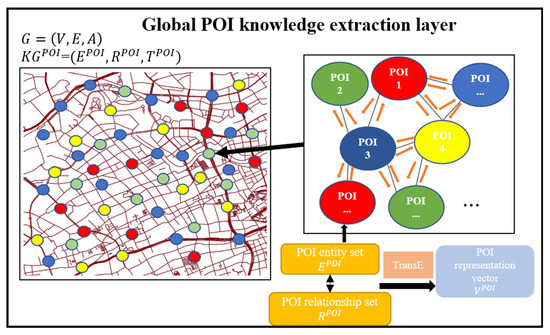
Figure 4. Global POI knowledge extraction layer.

As shown in Figure 4, the normalized POI was considered as the entity, and the link between the normalized POI was considered as the relationship, which in this paper denotes that there was a connection between two POI nodes. Moreover, the triplet $T^{POI}=\left\{\right(h,l,t\left)\right\}$ was considered as the training set of TransE algorithm, where $h$ represented the head entity, $t$ represented the tail entity, and $l$ represented the relationship; $h$ and $t$ belongs to the entity set $E^{POI}$, and $l$ belongs to the relationship set $R^{POI}$. The target of the TransE algorithm was to consider the relationship as the translation from the head entity to the tail entity, or to say, to made $h+l$ equal to $t$ as much as possible. The potential energy of a triplet is defined by the L2 norm of the difference between $h+l$ and $t$, as shown in Formula (5), where $N$ is the number of the triplets, and $i$ represents the triplet $i$.

$$\begin{array}{c}f\left(h_i,l_i,t_i\right)={\left|\left|h_i+l_i-t_i\right|\right|}_2=\sqrt{{\displaystyle \sum _{i=1}^N}{\left(h_i+l_i-t_i\right)}^2}\end{array}$$

(5)

Wrong triplets were identified and considered as negative samples in TransE algorithm for uniform sampling. A negative sample was generated when any one of the factors in a positive sample was replaced by the other entities or relationship randomly. The potential energy of the positive samples was reduced, and the potential energy of the negative samples were increased in the TransE algorithm. The objective function is defined in Formula (6).

$$\begin{array}{c}L={\displaystyle \sum _{\left(h,l,t\right)\in ∆}}{\displaystyle \sum _{\left(h^{\prime },l^{\prime },t^{\prime }\right)\in {∆}^{\prime }}}{\left[\left(f_r\left(h,t\right)+\gamma -f_{r^{\prime }}\left(h^{\prime },t^{\prime }\right)\right)\right]}_{+}\end{array}$$

(6)

where $∆$ is the set of positive samples, and ${∆}^{\prime }$ is the set of negative samples. $\gamma$ is a constant, usually is set as 1, which represents the distance between positive and negative samples. $(h,l,t)$ and $(h^{\prime },l^{\prime },t^{\prime })$ are the triplets of positive and negative samples, respectively. $f(·)$ is the potential energy function and ${[·]}_{+}$ is $max(0,·)$.

The distributed representation vector of the current head and tail entities were considered as the representation vectors ${V^{POI}}_{ij}\in {\mathbb{R}}^d$. The pseudocode of the global POI knowledge extraction layer is shown in Algorithm 1.

Algorithm 1: Global POI knowledge extraction layer
Input$\mathrm{entity}, \mathrm{relation}, \mathrm{and} \mathrm{training} \mathrm{sets} E^{POI},R^{POI},T^{POI}=\left\{\right(h,l,t\left)\right\}$$, \mathrm{embedding} \dim k$
1:	normalize $l\leftarrow$$\mathrm{uniform} (-\frac{6}{\sqrt{k}},\frac{6}{\sqrt{k}})$$\mathrm{for} \mathrm{each} l\in R^{POI}$
2:	$l/‖l‖$$\mathrm{for} \mathrm{each} l\in R^{POI}$
3:	$e\leftarrow$$\mathrm{uniform} (-\frac{6}{\sqrt{k}},\frac{6}{\sqrt{k}})$$\mathrm{for} \mathrm{each} e\in E^{POI}$
4:	loop
5:	$e/‖e‖$$\mathrm{for} \mathrm{each} e\in E^{POI}$
6:	$S_{batch}^{POI}\leftarrow$$\mathrm{sample} (T^{POI},b)$$//\mathrm{sample} \mathrm{by} \mathrm{size} b$
7:	$T_{batch}^{POI}\leftarrow \varnothing$  //initialize the triplets
8:	for $(h,l,t)\in S_{batch}^{POI}$ do
9:	$(h^{\prime },l^{\prime },t^{\prime })\leftarrow$$\mathrm{sample} {S^{\prime }}_{(h,l,t)}^{POI}$ //extract negative samples
10:	$T_{batch}^{POI}\leftarrow T_{batch}^{POI}\cup \left\{\left(\left(h,l,t\right),\left(h^{\prime },l^{\prime },t^{\prime }\right)\right)\right\}$ //extract positive and negative samples randomly
11:	end for
12:	$\mathrm{Update} \mathrm{embeddings} \sum _{\left(h,l,t\right)\in ∆}\sum _{\left(h^{\prime },l^{\prime },t^{\prime }\right)\in {∆}^{\prime }}{\left[\left(f_r\left(h,t\right)+\gamma -f_{r^{\prime }}\left(h^{\prime },t^{\prime }\right)\right)\right]}_{+}$ //L
13:	end loop
Output$\mathrm{representation} \mathrm{vector} V_{ij}^{POI}$ of the current entity

4.4. Local Dynamic Graph Generation Module

Local graphs were generated for each trajectory point in the local dynamic graph generation module. The Graph Attention network (GAT) was used as a spatial attention mechanism to allocate weight and update the parameters of every trajectory point and its neighbors. Corresponding graph representation vector ${NRV}_{ij}$ can be obtained through GAT.

As shown in Figure 5, every node in the global graph was embedded with the POI representation vector ${V^{POI}}_{ij}$ based on the POI knowledge graph in Section 4.3. The feature matrix $F\in {\mathbb{R}}^{N\times k}$ was constructed by all the embeddings of nodes, $F_{ij}={V^{POI}}_{ij}$, where $N$ is the number of the graph nodes, $k$ is the embedding dimension of the feature, $F_{ij}$ represents the feature matrix of the trajectory point $j$ of the trajectory $T_i$. The related local graphs ${G^{\prime }}_{ij-t:j}=(V_{ij-t:j},E_{ij-t:j},{A^{\prime }}_{ij-t:j})$ were generated for each normalized trajectory point $N{P}_{ij-t:j}$ in the normalized trajectory $N{T}_i$, where $V_{ij}$ is the set of the current point $N{P}_{ij}$ and its neighbor nodes, $E_{ij}$ is the set of edges among the current point and its neighbors, ${A^{\prime }}_{ij}$ is the local adjacency matrix of the current point, and it concludes the features of both the current point and its neighbor nodes.

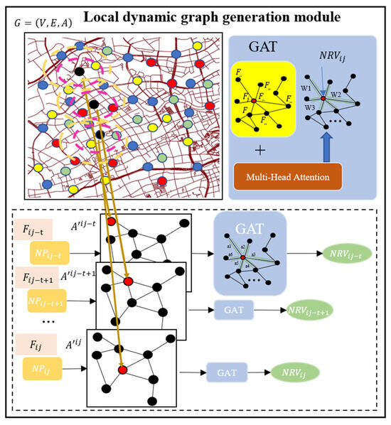
Figure 5. Local graph generation module.

GAT was used to calculate the attention weight between the trajectory points and their neighbor nodes and fused the features for the local graphs. The adjacency matrix was used to check whether there is a connection among nodes, and the resource was allocated by calculating the weights of the neighbor nodes in GAT. It can be considered as a spatial attention mechanism to enhance the interpretability of the proposed model. The definition of attention mechanism is shown as Formula (7).

$$\begin{array}{c}Attention\left(query,source\right)=\sum similarity\left(query,{key}_m\right)\ast {value}_m\end{array}$$

(7)

where $source$ is the original information, and it is formed by the $key–value$ pairs. $Attention\left(query,source\right)$ represents the information extraction through weight allocation from the $source$ under the condition of $query$. The aim of the GAT is to learn the relevance among target nodes and their neighbor nodes through the parameter matrix. In this paper, $query$ is set as the feature vector $F_{ij}$ of the current point $N{P}_{ij}$, $source$ is set as the feature vectors of all the neighbor nodes of $N{P}_{ij}$, ${key}_m$ and ${value}_m$ are, respectively, the $m^{th}$ neighbor node and its feature vector. The relevance coefficients among every trajectory point and its neighbor nodes were calculated in GAT. The calculation is shown in Formula (8).

$$\begin{array}{c}{e}_{jm}=LeakyReLU\left(w^T\left[W{F}_{ij}\right|\left|W{F}_{jm}\right]\right)\end{array}$$

(8)

where $\left|\right|$ represents concatenation, $F_{ij}$ is the feature vector of the point $j$ of the trajectory $T_i$, and $F_{jm}$ is the feature vector of the neighbor node $m$ of the point $j$. $W$ is a learnable weight parameter. $w$ is a learnable weight of the linear layer and $LeakyReLU$ is the activation function. Moreover, all the coefficients were normalized by the function $softmax$ in GAT to obtain the attention weight, as shown in Formula (9). $a_{jm}$ is the attention weight between node $j$ and its neighbor node $m$, where ${\mathcal{N}}_{ij}$ denotes the neighborhood of node $j$ in the trajectory $T_i$.

$$\begin{array}{c}{a}_{jm}=softmax\left(e_{jm}\right)=\frac{\exp \left(e_{jm}\right)}{\sum _{n\in {\mathcal{N}}_{ij}}\exp \left(ejn\right)}\end{array}$$

(9)

The aggregated and updated feature vector was then calculated, as shown in Formula (10). A multi-head attention mechanism was used to enhance the feature fusion of the neighbor nodes.

$$\begin{array}{c}{NPV}_{ij}={\left|\right|}_{h=1}^{H_1}\sigma \left({\sum }_{m\in {\mathcal{N}}_{ij}}{a_{jm}}^{\left(h\right)}{W}^{\left(h\right)}{F}_{jm}\right)\end{array}$$

(10)

where $H_1$ is the number of the heads, $\sigma$ is the activation function and ${NPV}_{ij}$ is the graph representation vector. The pseudocode of the local dynamic graph generation module is shown in Algorithm 2.

Algorithm 2: Local dynamic graph generation module
Input$\mathrm{normalized} \mathrm{trajectory} \mathrm{points} N{P}_{ij-t:j}$$, \mathrm{POI} \mathrm{feature} \mathrm{vectors} F_{ij}=V_{ij}^{POI}$
1:	${G^{\prime }}_{ij-t:j}\leftarrow (V_{ij-t:j},E_{ij-t:j},{A^{\prime }}_{ij-t:j})$ for each trajectory point   // generate local graphs
2:	$\mathrm{Target} \mathrm{node} \mathrm{vector} F_{ij}\leftarrow V_{ij}$$\mathrm{and} \mathrm{neighbor} \mathrm{node} \mathrm{vector} F_{jm}\leftarrow V_{jm}$ // according to local graphs
3:	$e_{jm}\leftarrow LeakyReLU\left(w^T\left[W{F}_{ij}\right|\left|W{F}_{jm}\right]\right)$
4:	$a_{jm}\leftarrow softmax\left(e_{jm}\right)$
5:	weighted sum:
6:	for $h\le H_1$ do
7:	$NP{V}_{ij}\leftarrow NP{V}_{ij}\Vert \sigma \left({\sum }_{m\in {\mathcal{N}}_{ij}}{a_{jm}}^{\left(h\right)}{W}^{\left(h\right)}{F}_{jm}\right)$
8:	end for
Output$\mathrm{graph} \mathrm{representation} \mathrm{vector} NP{V}_{ij}$ for each trajectory point

4.5. Trajectory Prediction Layer

In the trajectory prediction layer, trajectory points and corresponding graph representation vectors were input, and the coordinate of the next location were obtained after going through LSTM with a multi-head attention mechanism, as shown in Figure 6.

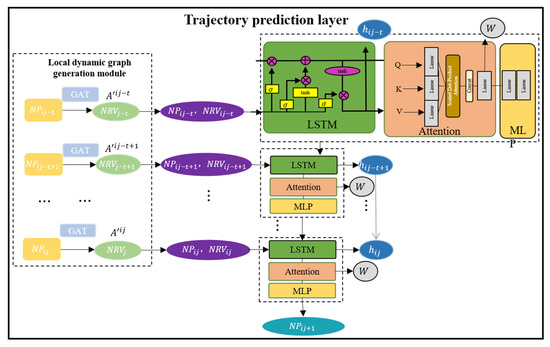
Figure 6. The research framework of the trajectory prediction layer.

As shown in Figure 6, the trajectory points $N{P}_{ij-t:j}$ and the corresponding graph representation vectors ${NPV}_{ij-t:j}$ were concatenated and input into LSTM, as shown in Formulas (11)–(17).

$$\begin{array}{c}{x}_j=\left\{N{P}_{ij},{NPV}_{ij}\right\}\end{array}$$

(11)

$$\begin{array}{c}{f}_j=\sigma \left(W_f·\left[h_{ij-1},x_j\right]+b_f\right)\end{array}$$

(12)

$$\begin{array}{c}{i}_j=\sigma \left(W_i·\left[h_{ij-1},x_j\right]+b_i\right)\end{array}$$

(13)

$$\begin{array}{c}{\tilde{C}}_j=\tanh \left(W_C·\left[h_{ij-1},x_j\right]+b_C\right)\end{array}$$

(14)

$$\begin{array}{c}{o}_j=\sigma \left(W_o·\left[h_{ij-1},x_j\right]+b_o\right)\end{array}$$

(15)

$$\begin{array}{c}{C}_j=f_j\ast C_{j-1}+i_j\ast {\tilde{C}}_j\end{array}$$

(16)

$$\begin{array}{c}{h}_{ij}=o_j\ast \tanh \left(C_j\right)\end{array}$$

(17)

where $W_f$, $W_i$, $W_C$ and $W_o$ are, respectively, the weight of the forget gate, the input gate, the cell state, and the output gate. $b_f$, $b_i$, $b_C$ and $b_o$ are the respective bias. The trajectory points and corresponding graph representation vectors were concatenated as the input $x_j$, as shown in Formula (11). $x_j$ goes through the forget, input, and output gates, and generate the cell state $C_j$, as shown in Formulas (12) and (13). Necessary information was processed by the input gate and the updated information was activated by the function $tanh$ to obtain the ${\tilde{C}}_j$, as shown in Formula (14). The current cell state $C_j$ is shown in Formula (16), where $f_j$ and $i_j$ are, respectively, the output of the forget gate and the input gate. $C_{j-1}$ is the cell state of the previous vector and ${\tilde{C}}_j$ is the activated state updated by the input gate. The hidden state $h_{ij}$ of the current vector is obtained by multiplying the activated cell state $C_j$ and the output of the output gate $o_j$, as shown in Formula (17).

A multi-head attention mechanism was used based on LSTM to allocate weight and enhance the interpretability of the proposed model, as shown in Formulas (18) and (19).

$$\begin{array}{c}{A}_h\left(Q_h,K_h,V_h\right)=softmax\left(\frac{Q_h{{·K}_h}^T}{\sqrt{d}}\right)V_h\end{array}$$

(18)

$$\begin{array}{c}MultiAtt\left(Q,K,V\right)=\left(A_1\left|\right|\dots \left|\right|A_{H_2}\right)W^O\end{array}$$

(19)

where $Q_h=W_i^Q{h}_{ij}$, $K_h=W_i^K,h_{ij-t:j}$, $V_h=W_i^V{h}_{ij-t:j}$. $h_{ij}$ is the hidden state of the current vector and is considered as the query, $h_{ij-t:j}$ denotes the hidden states of the vectors $x_{j-t:j}$ and is considered as the key and value, $W_i^Q$, $W_i^K$, $W_i^V$, $W^O$ are learnable weight parameters, $d$ is the dimension, and $H_2$ is the number of the heads.

The predicted result was obtained by adding a multilayer perceptron composed of two full-connected layers, as shown in Formula (20).

$$\begin{array}{c}{\widehat{Y}}_j=W_F^{2}ReLU\left(W_F^1{h_j}^{\prime }+b_F^1\right)+b_F^2\end{array}$$

(20)

where ${\widehat{Y}}_j$ is the predicted result. $W_F^1$, ${W_F^2}^{\prime }$, $b_F^1$, and $b_F^2$ are, respectively, the weights and biases of the two fully connected layers. ${h_j}^{\prime }$ is the output calculated by using the multi-head attention mechanism. Mean Square Error (MSE) was considered as the loss function to calculate the difference between the predicted results and truth, where $N$ is the number of trajectories and $K$ is the length of the trajectory. The calculation is shown in Formula (21).

$$\begin{array}{c}L={\displaystyle \sum _{i=1}^N}{\displaystyle \sum _{j=1}^K}{\left({\widehat{Y}}_j-{NP}_{ij}\right)}^2\end{array}$$

(21)

The pseudocode of the trajectory prediction layer is shown in Algorithm 3.

Algorithm 3: Trajectory prediction layer
Input$\mathrm{trajectory} \mathrm{points} \mathrm{in} \mathrm{normalization} \mathrm{form} N{P}_{ij-t:j}$$, \mathrm{representation} \mathrm{vectors} \mathrm{of} \mathrm{graph} NP{V}_{ij-t:j}$
1:	LSTM Module:
2:	loop
3:	$x_j\leftarrow \{N{P}_{ij},NP{V}_{ij}\}$
4:	$f_j,i_j,\widetilde{C_j},o_j\leftarrow$ calculated by forget gate, input gate and output gate
5:	$C_j,h_{ij}\leftarrow$$\mathrm{cell} \mathrm{state} \mathrm{and} \mathrm{hidden} \mathrm{state} \mathrm{are} \mathrm{calculated} \mathrm{by} f_j,i_j,\widetilde{C_j},o_j$
6:	Temporal attention mechanism:
7:	$Q_h\leftarrow W_i^Q h_{ij}$$, K_h\leftarrow W_i^K, h_{ij-t:j}$, $V_h\leftarrow W_i^V{h}_{ij-t:j}$
8:	for $h\le H_2$ do
9:	$A_h\leftarrow softmax\left(\frac{Q_h{{·K}_h}^T}{\sqrt{d}}\right)V_h$
10:	${h_j}^{\prime }\leftarrow {h_j}^{\prime }\Vert A_h{W}^O$
11:	end for
12:	MLP:
13:	${\widehat{Y}}_j\leftarrow W_F^{2}ReLU\left(W_F^1{h_j}^{\prime }+b_F^1\right)+b_F^2$
14:	end loop
Output$\mathrm{coordinate} {\widehat{Y}}_j$ of the next location

5. Experiments

This section will demonstrate the details of the experiments, including datasets, experiment settings and result analysis. The experiments were conducted to analyze the accuracy and robustness of the proposed model by comparing the performances with the benchmarks. Additionally, the ablation experiment was set to explore the effectiveness of the proposed model by filtering the spatial and temporal attention mechanisms. Moreover, the POI weights that influence the prediction results are visualized on the map to demonstrate the significance of urban functional regions to vehicle trajectories.

5.1. Datasets

Trajectory data: This study utilized Chengdu taxi trajectory data from Didi Gaiya, specifically from October 2018 and August 2014. The dataset includes attributes such as driver ID, order ID, timestamp, longitudes, and latitudes. Despite covering trajectory data for a single month, the dataset comprises over 380,000 trajectories generated by 14,000 vehicles. Notably, 270,000 trajectories are generated on holidays, while 110,000 pertain to working days. In terms of data distribution, the dataset predominantly covers the urban area of Chengdu, spanning from 30.65283 to 30.72649° N and 104.04210 to 104.12907° E. Each trajectory in the dataset has a sampling frequency of 4 s, resulting in a relatively high data density on the city road network. Given the dataset’s substantial volume, comprehensive distribution, and frequent sampling, it provides sufficient data to effectively train the proposed model presented in this paper.

Road Network data: The integration of Point of Interest (POI) and trajectory information forms the basis for constructing a comprehensive global traffic graph. The road network data for Chengdu were obtained from a map website OpenStreetMap (OSM). The node vector data include the road node ID along with its corresponding longitude and latitude. Each piece of road vector data comprises the road ID and a sequence of node coordinates defining its path.

POI data: 11 types of POI data concerning Chengdu from AutoNavi map were sourced through the Chinese Software Developer Network (CSDN) website. The original data format includes information such as POI name, longitude and latitude coordinates, address, district, and POI categories.

5.2. Experimental Settings

The experimental setup in this study is detailed as follows: The experiment employed AMD RYZEN 75,800 h CPU and Nvidia Geforce RTX 3060 GPU. The operating system was Windows 10, with Python as the coding language and PyTorch as the deep learning framework. Furthermore, the parameter configurations are outlined as follows: All models utilized a division of input data into training, validation, and test sets in a ratio of 7:2:1. A batch size of 16 was set, with an initial learning rate of 0.0001. The training process employed Adam as the optimizer. To ensure model convergence, the number of iterations was set to 17,500.

5.2.1. Benchmark Models

There are five baselines used in experiments for the comparation and evaluation of the proposed model, including LSTM [35], GRU [36], BiLSTM [37], AttnLSTM [38], and AttnBiLSTM [39].

LSTM: It is commonly employed in time series prediction. In contrast to traditional RNN models, LSTM addresses a deficiency where conventional models only factor in recent states and struggle with long-term memory. LSTM achieves this by utilizing an internal cell state and a forget gate, allowing it to decide which states to retain or forget. Additionally, it can circumvent certain gradient vanishing issues inherent in traditional RNN models.

GRU: It features only two gates and three fully connected layers in contrast to LSTM, leading to a reduction in computational requirements and lowering the overfitting risk. GRU incorporates an update and a reset gate, allowing it to regulate information output, selectively retaining historical information while discarding irrelevant data.

BiLSTM: Building upon LSTM, BiLSTM incorporates both forward and backward propagation in its input, enabling each timestamp in the input sequence to retain both future and past historical information simultaneously.

AttnLSTM: The attention mechanism is designed to allocate more weight to crucial tasks when computational resources are constrained in this model, acting as a resource allocation scheme to address information overload. Integrating LSTM with the attention mechanism enhances its performance by amplifying the importance of key features or filtering out irrelevant feature information.

AttnBiLSTM: BiLSTM combined with the attention mechanism can fuse information, which involves elevating the weight of significant features and employing bi-directional propagation. This integration enhances the computational efficiency and accuracy of the model by incorporating abundant semantic information.

5.2.2. Evaluation Metrics

Evaluation metrics used in this paper are Mean Absolute Error (MAE), Mean Square Error (MSE), Root Mean Square Error (RMSE), Haversine Distance (HSIN), and Accuracy. The definitions and equations of the five metrics are shown as follows. $Y_i$ denotes the ground truth and ${\widehat{Y}}_i$ denotes the predicted location, and the number of trajectory data for evaluation is denoted as $N$.

Mean Absolute Error (MAE): It denotes the mean of the absolute error between the value that was predicted and the actual value, which can be calculated as in Formula (22).

$$\begin{array}{c}\mathrm{MAE}=\frac{1}{N}{\displaystyle \sum _{i=1}^N}\left|Y_i-{\widehat{Y}}_i\right|\end{array}$$

(22)

Mean Square Error (MSE): This metric denotes the square of the variation between the ground truth and forecasted values, which can be calculated as in Formula (23).

$$\begin{array}{c}\mathrm{MSE}=\frac{1}{\mathrm{N}}{\displaystyle \sum _{\mathrm{i}=1}^{\mathrm{N}}}{\left({\mathrm{Y}}_{\mathrm{i}}-{\widehat{\mathrm{Y}}}_{\mathrm{i}}\right)}^2\end{array}$$

(23)

Root Mean Square Error (RMSE): The standard deviation of the difference between the ground truth and predicted results is RMSE. The model fits better if the RMSE is less. When it comes to high disparities, RMSE has greater penalties than MAE. It can be calculated as Formula (24), where $\mathrm{S}\mathrm{S}\mathrm{E}=\sum _{\mathrm{i}=1}^{\mathrm{N}}{({\mathrm{Y}}_{\mathrm{i}}-{\widehat{\mathrm{Y}}}_{\mathrm{i}})}^2$ denotes the squares of the error of all the samples.

$$\begin{array}{c}\mathrm{RMSE}=\sqrt{\mathrm{M}\mathrm{S}\mathrm{E}}=\sqrt{\frac{\mathrm{S}\mathrm{S}\mathrm{E}}{N}}=\sqrt{\frac{1}{N}{\displaystyle \sum _{i=1}^N}{\left(Y_i-{\widehat{Y}}_i\right)}^2}\end{array}$$

(24)

Haversine Distance (HSIN): This metric denotes the distance between the actual and predicted locations. The model with lower distance error is better. It can be calculated as shown in Formula (25), where $Y_i=\left({lat}_i,{lon}_i\right)$ is the truth and ${\widehat{Y}}_i=\left({\widehat{lat}}_i,{\widehat{lon}}_i\right)$ is the predicted longitude and latitude.

$$\begin{array}{c}\mathrm{HSIN}=2r argsin\left(\sqrt{{sin}^2\left(\frac{{lat}_i-{\widehat{lat}}_i}{2}\right)+\cos \left({lat}_i\right)\cos \left({\widehat{lat}}_i\right){sin}^2\left(\frac{{lon}_i-{\widehat{lon}}_i}{2}\right)}\right)\end{array}$$

(25)

Accuracy: It indicates the proportion of the accurately predicted output in the total output. The higher the accuracy rate, the better the model training effect. It can be calculated as shown in Formula (26), and $TP$ denotes the correctly predicted results, $NP$ denotes the incorrectly predicted results, and $count(·)$ denotes the counting number.

$$\begin{array}{c}\mathrm{Accuracy}=\frac{count\left(TP\right)}{count\left(TP\right)+count\left(NP\right)} \end{array}$$

(26)

5.3. Result Analysis

The accuracy experiment and the robustness experiment are discussed in this paper. The LDGST-LSTM model is compared with the benchmark models to explore the performance in terms of accuracy and robustness. The ablation experiment is discussed to verify the spatial and temporal attention mechanisms of the proposed model to enhance interpretability. Moreover, the POI weights calculated using the temporal attention mechanism are visualized on the map. The POI is considered as the feature of the vehicle trajectory, and the influence of the POI on vehicle position prediction is revealed.

5.3.1. Accuracy Experiment

All models were trained, and the accuracy comparison results on the training set are shown in Figure 7. It can be seen that on both holidays and working days, the accuracy of LDGST-LSTM was significantly higher than the benchmarks.

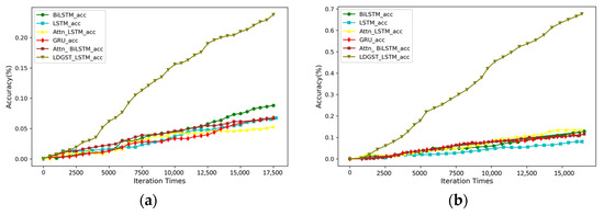
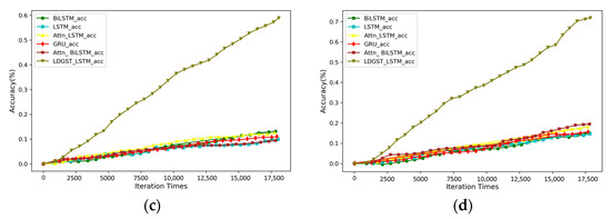
Figure 7. Accuracy comparison of different models on training set: (a) holidays in October 2018, (b) working days in October 2018, (c) weekends in August 2014, and (d) working days in August 2014.

As shown in Figure 7a,b, the accuracy of the proposed model on both holidays and working days was nearly 4.5 times higher than the benchmarks in the dataset of October 2018. As shown in Figure 7c,d, the accuracy of the proposed model on both weekends and working days was nearly 3.5–4.5 times higher than the benchmarks in the dataset of August 2014. Therefore, the accuracy of location prediction can be effectively improved by considering POI knowledge and combining GAT and temporal attention mechanisms.

The accuracy comparison results of different models are shown in Table 1.

Table 1. Accuracy comparison of different models on holidays in October 2018, working days in October 2018, weekends in August 2014, and working days in August 2014.

	Accuracy in October 2018 (%)		Accuracy in August 2014 (%)
Model	on Holidays	on Working Days	on Weekends	on Working Days
LSTM	0.09	0.10	0.12	0.10
GRU	0.07	0.08	0.12	0.07
BiLSTM	0.06	0.07	0.11	0.05
Attn-LSTM	0.05	0.14	0.15	0.09
Attn-BiLSTM	0.06	0.09	0.16	0.05
LDGST-LSTM	0.30	0.75	0.80	0.57

In the October 2018 dataset, the accuracy of LDGST-LSTM was 21% higher compared to LSTM during holidays and 61% higher compared to Attn-LSTM during weekdays. In the August 2014 dataset, LDGST-LSTM improved by 64% compared to Attn-BiLSTM on weekends. Therefore, compared to the benchmarks, the model proposed in this paper can improve performance by selecting appropriate POI categories on weekdays and holidays, respectively. More importantly, integrating POI knowledge and combining spatial and temporal attention mechanisms can greatly improve the accuracy of vehicle trajectory location prediction.

5.3.2. Robustness Experiment

The results of the robustness experiment are discussed in this section. The convergence speed and the metrics after convergence of the proposed model and benchmarks are compared to analyze the robustness. The results of convergence speed are shown in Figure 8.

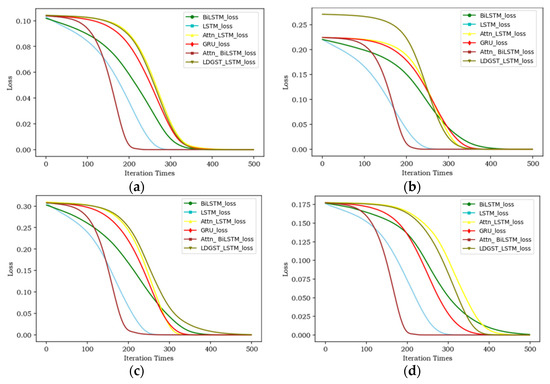
Figure 8. Convergence speed comparison of different models: (a) holidays in October 2018, (b) working days in October 2018, (c) weekends in August 2014, and (d) working days in August 2014.

As shown in Figure 8a,b, the loss of LDGST-LSTM drops slowly compared with the benchmark models before the 200th iteration on the dataset of October 2018. The convergence speed of the proposed model becomes faster from the 250th to the 300th iterations, and it converges at around the 350th iteration. As shown in Figure 8c,d, the loss of LDGST-LSTM drops slowly compared with the benchmark models before the 200th iterations on the dataset of August 2014. Additionally, the convergence speed of the proposed model becomes faster from the 250th to the 350th iterations and it converges at around the 450th iteration.

The performance of MAE, MSE, RMSE and HISN of different models are shown in Table 2, Table 3, Table 4 and Table 5. As shown in Table 2 and Table 3, the performance of the proposed model on evaluation metrics was the best compared with benchmarks when using the dataset of October 2018. The MAE, MSE, RMSE, and HSIN of the proposed model were, respectively, 7.73%, 28.57%, 11.11%, and 15.72% lower than LSTM, which was the most robust among the baselines in the holidays. The MAE, MSE, RMSE, and HSIN of the proposed model were, respectively, 6.19%, 33.33%, 27.27%, and 41.79% lower than GRU, which was the most robust among the benchmarks in the working days. As shown in Table 4 and Table 5, the performance of the proposed model on evaluation metrics were still the best when using the dataset of Chengdu August 2014. The four metrics of the proposed model were, respectively, 6.09%, 33.33%, 15.64%, and 41.66% lower than GRU in the weekend. The MAE, MSE, RMSE, and HSIN of the proposed model were, respectively, 4.88%, 28.57%, 18.55%, and 15.99% lower than LSTM in the working days. Therefore, it can be seen that the robustness of the proposed model were the best compared with all the benchmark models.

Table 2. Performance comparison of different models on holidays in October 2018.

Model	MAE	MSE	RMSE	HISN
LSTM	0.0207	0.0007	0.0234	2.4433
GRU	0.0218	0.0008	0.0243	2.8943
BiLSTM	0.0302	0.0012	0.0329	4.7287
Attn-LSTM	0.0234	0.0009	0.0258	3.7313
Attn-BiLSTM	0.0492	0.0035	0.0567	8.4362
LDGST-LSTM	0.0191	0.0005	0.0208	2.0591

Table 3. Performance comparison of different models on working days in October 2018.

Model	MAE	MSE	RMSE	HISN
LSTM	0.0212	0.0009	0.0295	3.5067
GRU	0.0210	0.0009	0.0275	3.4957
BiLSTM	0.0305	0.0010	0.0305	3.1503
Attn-LSTM	0.0220	0.0008	0.0250	3.4728
Attn-BiLSTM	0.0345	0.0012	0.0355	3.7504
LDGST-LSTM	0.0197	0.000	0.0200	2.0348

Table 4. Performance comparison of different models on weekends in August 2014.

Model	MAE	MSE	RMSE	HISN
LSTM	0.0202	0.0007	0.0305	2.9507
GRU	0.0197	0.0006	0.0275	2.6054
BiLSTM	0.0255	0.0008	0.0335	3.0504
Attn-LSTM	0.0199	0.0006	0.0290	2.6595
Attn-BiLSTM	0.0301	0.0012	0.0403	3.7955
LDGST-LSTM	0.0185	0.0004	0.0232	2.0634

Table 5. Performance comparison of different models on working days in August 2014.

Model	MAE	MSE	RMSE	HISN
LSTM	0.0205	0.0007	0.0275	2.5047
GRU	0.0227	0.0009	0.0294	2.8643
BiLSTM	0.0269	0.0011	0.0327	3.0457
Attn-LSTM	0.0235	0.0009	0.0310	3.0137
Attn-BiLSTM	0.0312	0.0014	0.0343	3.3189
LDGST-LSTM	0.0195	0.0005	0.0224	2.1042

5.3.3. Ablation Experiment

The ablation experiment is discussed to analyze the effect of major components in the proposed model by filtering GAT and the temporal attention mechanism. In addition to the proposed model, three ablation models are analyzed, including (1) Local Dynamic Graph Convolutional Network–Long Short-Term Memory (LDGCN-LSTM), (2) Local Dynamic Graph Convolutional Network–Temporal Attention Long Short-Term Memory (LDGCN-TAttnLSTM), and (3) Local Dynamic Graph Attention–Long Short-Term Memory (LDGAT-LSTM).

As shown in Figure 9, the accuracy of LDGST-LSTM is the highest among the other three ablation models in both datasets. The accuracy of LDGST-LSTM is almost the same as the accuracy of LDGAT-LSTM. It may be the reason that, during holidays, the intention of the taxis is more focused on some functional regions, and the importance of spatial overweighs the temporal features.

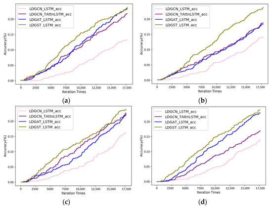
Figure 9. Accuracy comparison of different ablation modules: (a) holidays in October 2018, (b) working days in October 2018, (c) weekends in August 2014, and (d) working days in August 2014.

The ablation results are shown in Table 6, Table 7, Table 8 and Table 9. As shown in Table 6 and Table 7, the evaluation metrics of LDGST-LSTM were the best among the ablation models when using a dataset in 2018. The MAE, MSE, RMSE, and HSIN of the proposed model were, respectively, 9.91%, 28.57%, 12.97%, and 15.46% lower, and the accuracy was 4.17% higher than LDGAT-LSTM, which means it performed the best among ablation models in the holidays. The MAE, MSE, RMSE, and HSIN of the proposed model were, respectively, 3.9%, 14.29%, 22.18%, and 20.12% lower, and the accuracy was 40% higher than LDGAT-LSTM on working days. As shown in Table 8 and Table 9, the performances of LDGST-LSTM were also the best in the 2014 dataset. The four metrics of LDGST-LSTM were, respectively, 25.40%, 33.33%, 18.31% and 18.52% lower, and the accuracy was 7.69% higher than LDGAT-LSTM; therefore, it performed the best among ablation models in the weekends. The MAE, MSE, RMSE and HSIN of LDGST-LSTM were, respectively, 10.55%, 28.57%, 11.81% and 10.42% lower, and the accuracy was 3.64% higher than LDGAT-LSTM on working days. In conclusion, the proposed model performed the best compared with other ablation models. Therefore, the combination of GAT and temporal attention mechanism can enhance the interpretability and improve the accuracy and robustness of the model.

Table 6. Ablation results of the proposed model on holidays in October 2018.

Model	MAE	MSE	RMSE	HISN	Accuracy (%)
LDGST-LSTM	0.0191	0.0005	0.0208	2.0591	0.25
LDGAT-LSTM	0.0212	0.0007	0.0239	2.4357	0.24
LDGCN-TAttnLSTM	0.0225	0.0008	0.0244	2.6329	0.20
LDGCN-LSTM	0.0195	0.0005	0.0224	2.1042	0.13

Table 7. Ablation results of the proposed model on working days in October 2018.

Model	MAE	MSE	RMSE	HISN	Accuracy (%)
LDGST-LSTM	0.0197	0.0006	0.0200	2.0348	0.70
LDGAT-LSTM	0.0205	0.0007	0.0257	2.5473	0.50
LDGCN-TAttnLSTM	0.0220	0.0008	0.0295	2.6904	0.45
LDGCN-LSTM	0.0237	0.0010	0.0305	2.9754	0.40

Table 8. Ablation results of the proposed model on weekends in August 2014.

Model	MAE	MSE	RMSE	HISN	Accuracy (%)
LDGST-LSTM	0.0185	0.0004	0.0232	2.0634	0.70
LDGAT-LSTM	0.0253	0.0007	0.0301	2.8751	0.64
LDGCN-TAttnLSTM	0.0248	0.0006	0.0284	2.5323	0.65
LDGCN-LSTM	0.0297	0.0009	0.0328	2.9107	0.50

Table 9. Ablation results of the proposed model on working days in August 2014.

Model	MAE	MSE	RMSE	HISN	Accuracy (%)
LDGST-LSTM	0.0195	0.0005	0.0224	2.1042	0.57
LDGAT-LSTM	0.0218	0.0007	0.0254	2.3490	0.55
LDGCN-TAttnLSTM	0.0261	0.0009	0.0278	2.5983	0.40
LDGCN-LSTM	0.0284	0.0009	0.0290	2.9841	0.30

5.3.4. POI Weights Visualization

The predicted coordinates of the next location, along with their corresponding weight, can be calculated by using the proposed model. The visualization of POI weights is realized through the nuclear density analysis in the ArcGIS.

The visualization of POI weight has a positive significance in terms of vehicle trajectory planning, traffic optimization, and vehicle location prediction. As shown in Figure 10, there are some regions of POI information that affect vehicle location prediction. For example, this is shown in the western and southern regions in Figure 10a,c, and the right and the top sides in Figure 10b,d. It can be seen that on holidays and weekends, POI in the western and southern regions can be considered important information that influences vehicle trajectories. It may denote that these regions are close to the center of the city and have high traffic flow on holidays and weekends. Therefore, it is important to plan the driving path in these regions on holidays and weekends. Moreover, POI regions that influence the location prediction are more dispersed on working days, and the trajectory decision can be more flexible.

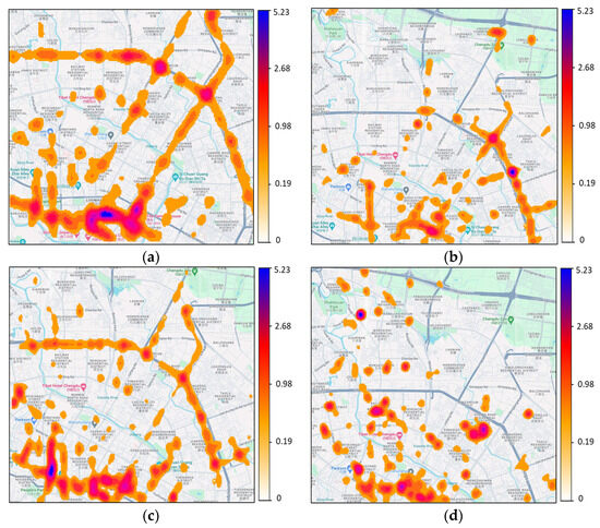
Figure 10. Visualization of the POI weights: (a) holidays in October 2018, (b) working days in October 2018, (c) weekends in August 2014, and (d) working days in August 2014.

6. Conclusions and Future Work

A Local Dynamic Graph Spatiotemporal–Long Short-Term Memory (LDGST-LSTM) model was proposed in this paper to predict the next location of vehicle trajectory. The data conversion layer, POI global knowledge extraction layer, local dynamic graph generation module, and trajectory prediction layer were major components of the proposed model. Raw taxi trajectory and POI semantic information were first matched to the road network through the use of a map-matching algorithm and proximity algorithm in the data conversion layer. Then, the representation vectors of POI were learned through the use of the TransE algorithm by constructing a knowledge graph in the POI global knowledge extraction layer. Based on the global knowledge graph, a local graph related to each trajectory point was generated, and the graph representation vector was captured through GAT in the local dynamic graph generation module. Finally, trajectory points with the related graph representation vectors were input into LSTM with a multi-head attention mechanism in the trajectory prediction layer to predict the next location.

However, there are limitations in this paper. Firstly, exploring accurate trajectory recovery can be a potential avenue for future research due to non-uniform GPS sampling and the presence of GPS signal shielding areas. Moreover, only POI knowledge is considered as the external feature in this paper. The current approach heavily relies on Points of Interest for contextual information. However, there may be other relevant contextual factors, such as real-time weather conditions and road construction, which could influence trajectory prediction. Exploring these factors can provide a more comprehensive understanding of the environment and enhance the accuracy and robustness of the model. Additionally, knowledge graphs are currently static and do not dynamically update in real time. This limitation may impact the model’s adaptability to changes in the environment, such as sudden road closures or new construction. Therefore, implementing a mechanism for online updating of knowledge graphs based on real-time data can be a further enhancement. This ensures that the model adapts dynamically to changes in the environment, improving its ability to handle dynamic scenarios. Moreover, scenarios in this paper were the macro traffic roads and specific traffic scenarios such as complex intersections and traffic light timing could be a challenge for trajectory prediction. The current model may struggle to accurately predict trajectories in scenarios where multiple roads converge or diverge. Therefore, further research could focus on developing specialized mechanisms for handling complex intersections. This may involve incorporating advanced spatial attention mechanisms or considering the historical behavior of vehicles at such intersections. In recent years, the rapid development of connected automated vehicles has significantly transformed the landscape of transportation. The emergence of shared data on the road presents a unique opportunity to enhance various aspects of vehicular technologies, including trajectory prediction. Leveraging data from connected vehicles, such as cooperative perception using 3D LiDAR [40], can indeed contribute valuable insights to trajectory dynamics. The potential of shared information from connected vehicles to revolutionize the accuracy and reliability of trajectory predictions can be another new direction for research and innovation. Furthermore, extending the analysis in terms of dataset duration and geographic coverage is another further research direction. Assessing the model’s performance over a more extended period should be considered, such as capturing potential variations in different seasons or temporal patterns. The effectiveness of the model across a broader geographic area should also be considered, incorporating diverse scenarios to test its adaptability in different environments.

References

- Guo, L. Research and Application of Location Prediction Algorithm Based on Deep Learning. Ph.D. Thesis, Lanzhou University, Lanzhou, China, 2018. [Google Scholar]
- Havyarimana, V.; Hanyurwimfura, D.; Nsengiyumva, P.; Xiao, Z. A novel hybrid approach based-SRG model for vehicle position prediction in multi-GPS outage conditions. Inf. Fusion 2018, 41, 1–8. [Google Scholar] [CrossRef]
- Wu, Y.; Hu, Q.; Wu, X. Motor vehicle trajectory prediction model in the context of the Internet of Vehicles. J. Southeast Univ. (Nat. Sci. Ed.) 2022, 52, 1199–1208. [Google Scholar]
- Li, L.; Xu, Z. Review of the research on the motion planning methods of intelligent networked vehicles. J. China Highw. Transp. 2019, 32, 20–33. [Google Scholar]
- Liao, J. Research and Application of Vehicle Position Prediction Algorithm Based on INS/GPS. Ph.D. Thesis, Hunan University, Hunan, China, 2016. [Google Scholar]
- Wang, K.; Wang, Y.; Deng, X. Review of the impact of uncertainty on vehicle trajectory prediction. Autom. Technol. 2022, 7, 1–14. [Google Scholar]
- Wang, L. Trajectory Destination Prediction Based on Traffic Knowledge Map. Ph.D. Thesis, Dalian University of Technology, Dalian, China, 2021. [Google Scholar]
- Guo, H.; Meng, Q.; Zhao, X. Map-enhanced generative adversarial trajectory prediction method for automated vehicles. Inf. Sci. 2023, 622, 1033–1049. [Google Scholar] [CrossRef]
- Xu, H.; Yu, J.; Yuan, S. Research on taxi parking location selection algorithm based on POI. High-Tech Commun. 2021, 31, 1154–1163. [Google Scholar]
- Velickovic, P.; Cucurull, G.; Casanova, A.; Romero, A.; Lio’, P.; Bengio, Y. Graph Attention Networks. arXiv 2017, arXiv:1710.10903. [Google Scholar]
- Li, L.; Ping, Z.; Zhu, J. Space-time information fusion vehicle trajectory prediction for group driving scenarios. J. Transp. Eng. 2022, 22, 104–114. [Google Scholar]
- Su, J.; Jin, Z.; Ren, J.; Yang, J.; Liu, Y. GDFormer: A Graph Diffusing Attention based approach for Traffic Flow Prediction. Pattern Recognit. Lett. 2022, 156, 126–132. [Google Scholar] [CrossRef]
- Ali, A.; Zhu, Y.; Zakarya, M. Exploiting dynamic spatio-temporal correlations for citywide traffic flow prediction using attention based neural networks. Inf. Sci. 2021, 577, 852–870. [Google Scholar] [CrossRef]
- Fan, H. Research and Implementation of Vehicle Motion Tracking Technology Based on Internet of Vehicles. Ph.D. Thesis, Beijing University of Posts and Telecommunications, Beijing, China, 2017. [Google Scholar]
- Hui, F.; Wei, C.; Shangguan, W.; Ando, R.; Fang, S. Deep encoder-decoder-NN: A deep learning-based autonomous vehicle trajectory prediction and correction model. Phys. A Stat. Mech. Its Appl. 2022, 593, 126869. [Google Scholar] [CrossRef]
- Kalatian, A.; Farooq, B. A context-aware pedestrian trajectory prediction framework for automated vehicles. Transp. Res. C Emerg. Technol. 2022, 134, 103453. [Google Scholar] [CrossRef]
- An, J.; Liu, W.; Liu, Q.; Guo, L.; Ren, P.; Li, T. DGInet: Dynamic graph and interaction-aware convolutional network for vehicle trajectory prediction. Neural Netw. 2022, 151, 336–348. [Google Scholar] [CrossRef]
- Zambrano-Martinez, J.L.; Calafate, C.T.; Soler, D.; Cano, J.C.; Manzoni, P. Modeling and characterization of traffic flows in urban environments. Sensors 2018, 18, 2020. [Google Scholar] [CrossRef]
- Zhang, X.; Onieva, E.; Perallos, A.; Osaba, E.; Lee, V. Hierarchical fuzzy rule-based system optimized with genetic algorithms for short term traffic congestion prediction. Transp. Res. C Emerg. Technol. 2014, 43, 127–142. [Google Scholar] [CrossRef]
- Yang, D.; He, T.; Wang, H. Research progress in graph embedding learning for knowledge map. J. Softw. 2022, 33, 21. [Google Scholar]
- Xia, Y.; Lan, M.; Chen, X. Overview of interpretable knowledge map reasoning methods. J. Netw. Inf. Secur. 2022, 8, 1–25. [Google Scholar]
- Zhang, Z.; Qian, Y.; Xing, Y. Overview of TransE-based representation learning methods. J. Comput. Appl. Res. 2021, 3, 656–663. [Google Scholar]
- Chen, W.; Wen, Y.; Zhang, X. An improved TransE-based knowledge map representation method. Comput. Eng. 2020, 46, 8. [Google Scholar]
- Zheng, D.; Song, X.; Ma, C.; Tan, Z.; Ye, Z.; Dong, J.; Xiong, H.; Zhang, Z.; Karypis, G. DGL-KE: Training Knowledge Graph Embeddings at Scale. In Proceedings of the SIGIR ′20: Proceedings of the 43rd International ACM SIGIR Conference on Research and Development in Information Retrieval, Virtual, 25–30 July 2020. [Google Scholar]
- Ji, Q.; Jin, J. Reasoning Traffic Pattern Knowledge Graph in Predicting Real-Time Traffic Congestion Propagation. IFAC-PapersOnLine 2020, 53, 578–581. [Google Scholar] [CrossRef]
- Wang, X.; Lyu, S.; Wang, X.; Wu, X.; Chen, H. Temporal knowledge graph embedding via sparse transfer matrix. Inf. Sci. 2022, 623, 56–69. [Google Scholar] [CrossRef]
- Wang, C.; Tian, R.; Hu, J.; Ma, Z. A trend graph attention network for traffic prediction. Inf. Sci. 2023, 623, 275–292. [Google Scholar] [CrossRef]
- Wang, B.; Wang, J. ST-MGAT:Spatio-temporal multi-head graph attention network for Traffic prediction. Phys. A-Stat. Mech. Its Appl. 2022, 603, 127762. [Google Scholar] [CrossRef]
- Wang, T.; Ni, S.; Qin, T.; Cao, D. TransGAT: A dynamic graph attention residual networks for traffic flow forecasting. Sustain. Comput. Inform. Syst. 2022, 36, 100779. [Google Scholar] [CrossRef]
- Cai, K.; Shen, Z.; Luo, X.; Li, Y. Temporal attention aware dual-graph convolution network for air traffic flow prediction. J. Air Transp. Manag. 2023, 106, 102301. [Google Scholar] [CrossRef]
- Yan, X.; Gan, X.; Wang, R.; Qin, T. Self-attention eidetic 3D-LSTM: Video prediction models for traffic flow forecasting. Neurocomputing 2022, 509, 167–176. [Google Scholar] [CrossRef]
- Chen, L.; Shi, P.; Li, G.; Qi, T. Traffic flow prediction using multi-view graph convolution and masked attention mechanism. Comput. Commun. 2022, 194, 446–457. [Google Scholar] [CrossRef]
- Wang, K.; Ma, C.; Qiao, Y.; Lu, X.; Hao, W.; Dong, S. A hybrid deep learning model with 1DCNN-LSTM-Attention networks for short-term traffic flow prediction. Phys. A-Stat. Mech. Its Appl. 2021, 583, 126293. [Google Scholar] [CrossRef]
- Lou, Y.; Zhang, C.; Zheng, Y.; Xie, X.; Wang, W.; Huang, Y. Map-matching for low-sampling-rate GPS trajectories. In Proceedings of the GIS ′09: Proceedings of the 17th ACM SIGSPATIAL International Conference on Advances in Geographic Information Systems, Seattle, WA, USA, 4–6 November 2009. [Google Scholar]
- Cai, Y. Research on Vehicle Trajectory Prediction Based on RNN-LSTM Network. Ph.D. Thesis, Jilin University, Jilin, China, 2021. [Google Scholar]
- Zhang, H.; Huang, C.; Xuan, Y. Real time prediction of air combat flight trajectory using gated cycle unit. Syst. Eng. Electron. Technol. 2020, 42, 7. [Google Scholar]
- Guo, Y.; Zhang, R.; Chen, Y. Vehicle trajectory prediction based on potential features of observation data and bidirectional long short-term memory network. Autom. Technol. 2022, 3, 21–27. [Google Scholar]
- Liu, C.; Liang, J. Vehicle trajectory prediction based on attention mechanism. J. Zhejiang Univ. (Eng. Ed.) 2020, 54, 8. [Google Scholar]
- Guan, D. Research on Modeling and Prediction of Vehicle Moving Trajectory in the Internet of Vehicles. Ph.D. Thesis, Beijing University of Posts and Telecommunications, Beijing, China, 2020. [Google Scholar]
- Meng, Z.; Xia, X.; Xu, R.; Liu, W.; Ma, J. HYDRO-3D: Hybrid Object Detection and Tracking for Cooperative Perception Using 3D LiDAR. IEEE Trans. Intell. Veh. 2023, 8, 4069–4080. [Google Scholar] [CrossRef]
Disclaimer/Publisher’s Note: The statements, opinions and data contained in all publications are solely those of the individual author(s) and contributor(s) and not of MDPI and/or the editor(s). MDPI and/or the editor(s) disclaim responsibility for any injury to people or property resulting from any ideas, methods, instructions or products referred to in the content. |
© 2024 by the authors. Licensee MDPI, Basel, Switzerland. This article is an open access article distributed under the terms and conditions of the Creative Commons Attribution (CC BY) license (https://creativecommons.org/licenses/by/4.0/).