
Towards Efficient Battery Electric Bus Operations: A Novel Energy Forecasting Framework


Abstract
1. Introduction
- Can data-driven approaches improve energy forecasting for battery electric buses over constant value assumption for practical applications?
- How big is the error margin for data-driven models versus constant values?
- How can bus operators benefit from more precise energy forecasting?
2. Background and Motivation
2.1. Data Analysis in BEB Operations
2.2. Predictive Models for BEB Energy Consumption
2.3. Simulation Approaches for BEB Energy Prediction
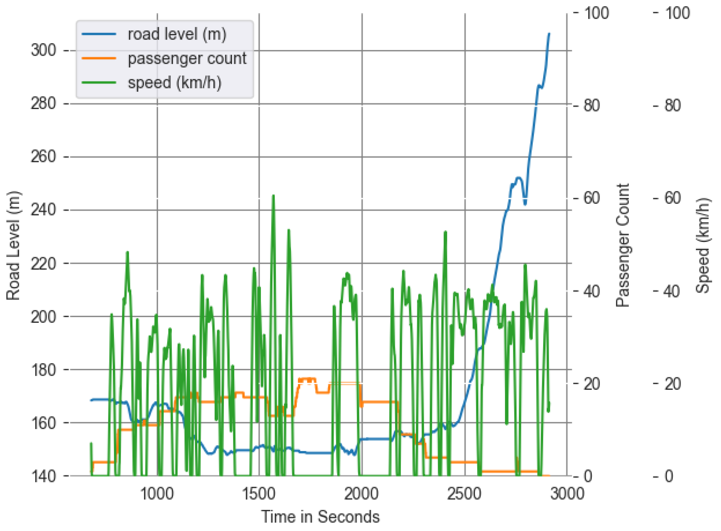
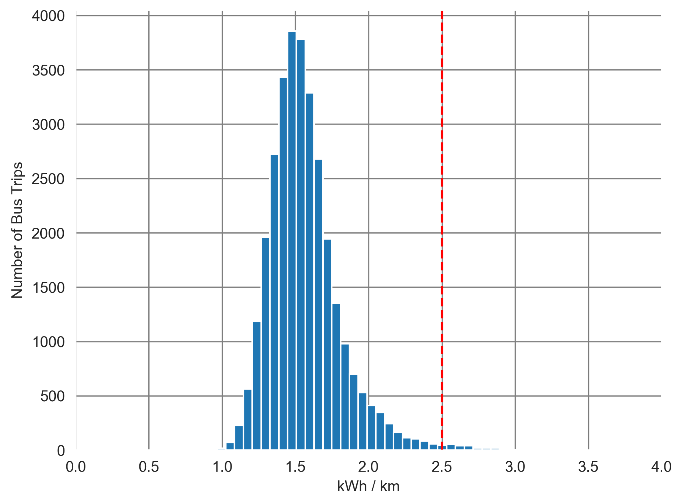
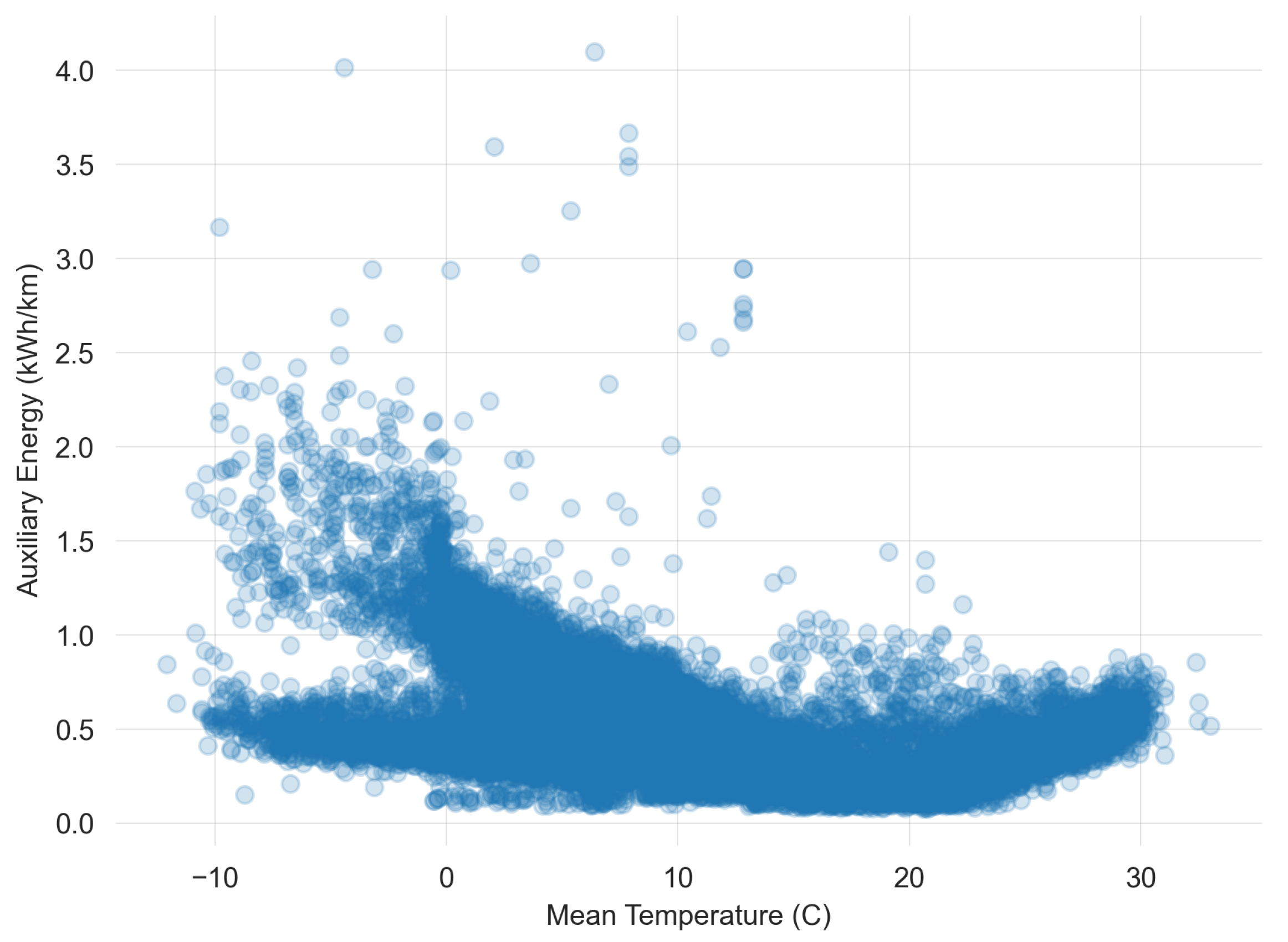
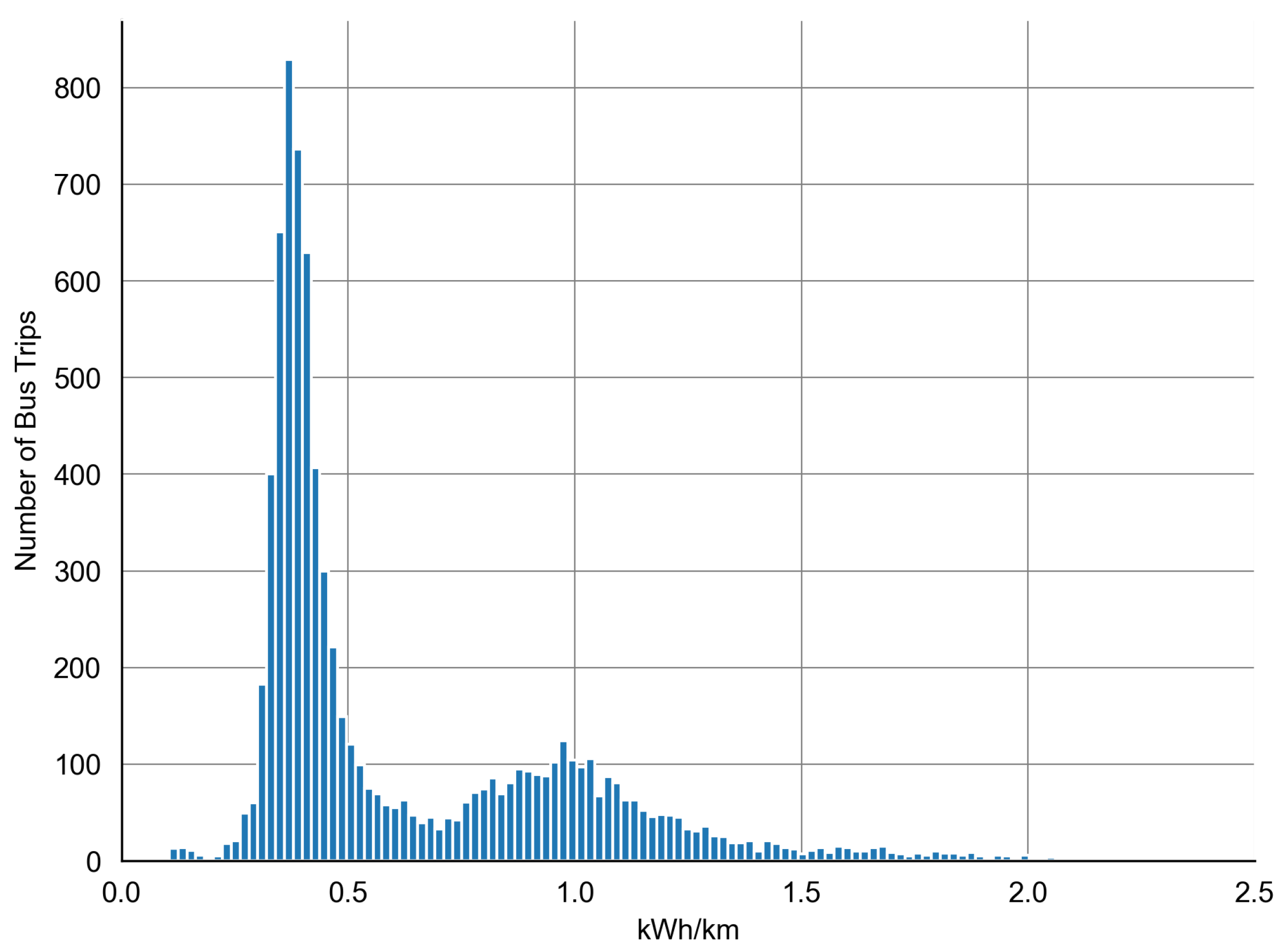
3. Data Analysis
3.1. Data Collection and Preprocessing
3.2. Basic Numbers
- Total Trips Observed: The analysis is based on 46,675 bus trips from 16 vehicles over 13 months. From November 2022 to November 2023.
- Total Electrical Energy: A cumulative consumption of 619 MWh was recorded.
- Auxiliary Energy: Auxiliary systems accounted for 176 MWh, 28.5% of the total consumption. This appears to be quite high considering the additional diesel heating for cold conditions.
- Passenger Kilometers: The buses covered 6.82 million passenger kilometers (pkm).
- Electrical Energy per Passenger Kilometer (kWh/pkm): The average consumption was 0.09 kWh per passenger kilometer.
- Temperature Range: Operational temperatures varied from −12 °C to 33 °C.
- Passenger Volume: The average number of passengers was around 19, occasionally exceeding the maximum capacity of 145 passengers during peak hours.
3.3. Influencing Factors
3.3.1. Elevation Gain
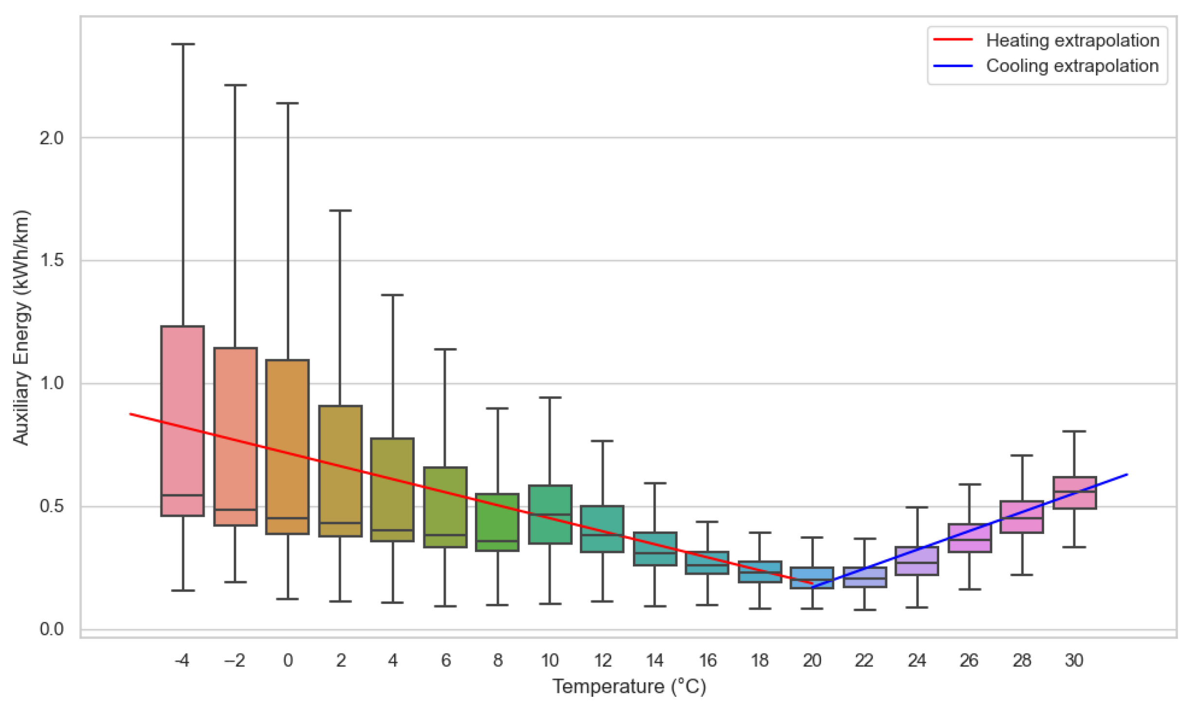
3.3.2. Temperature
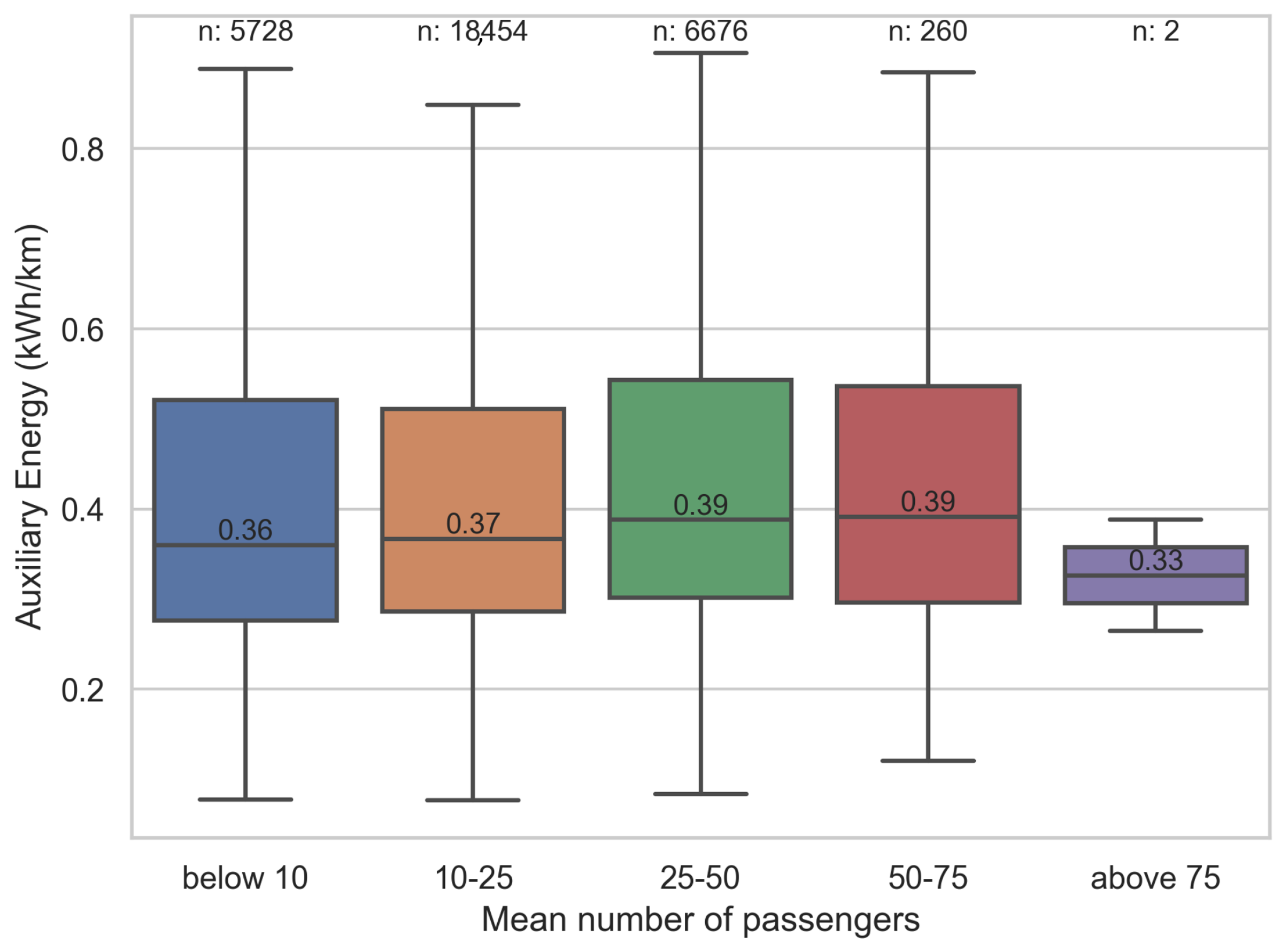
3.3.3. Passengers
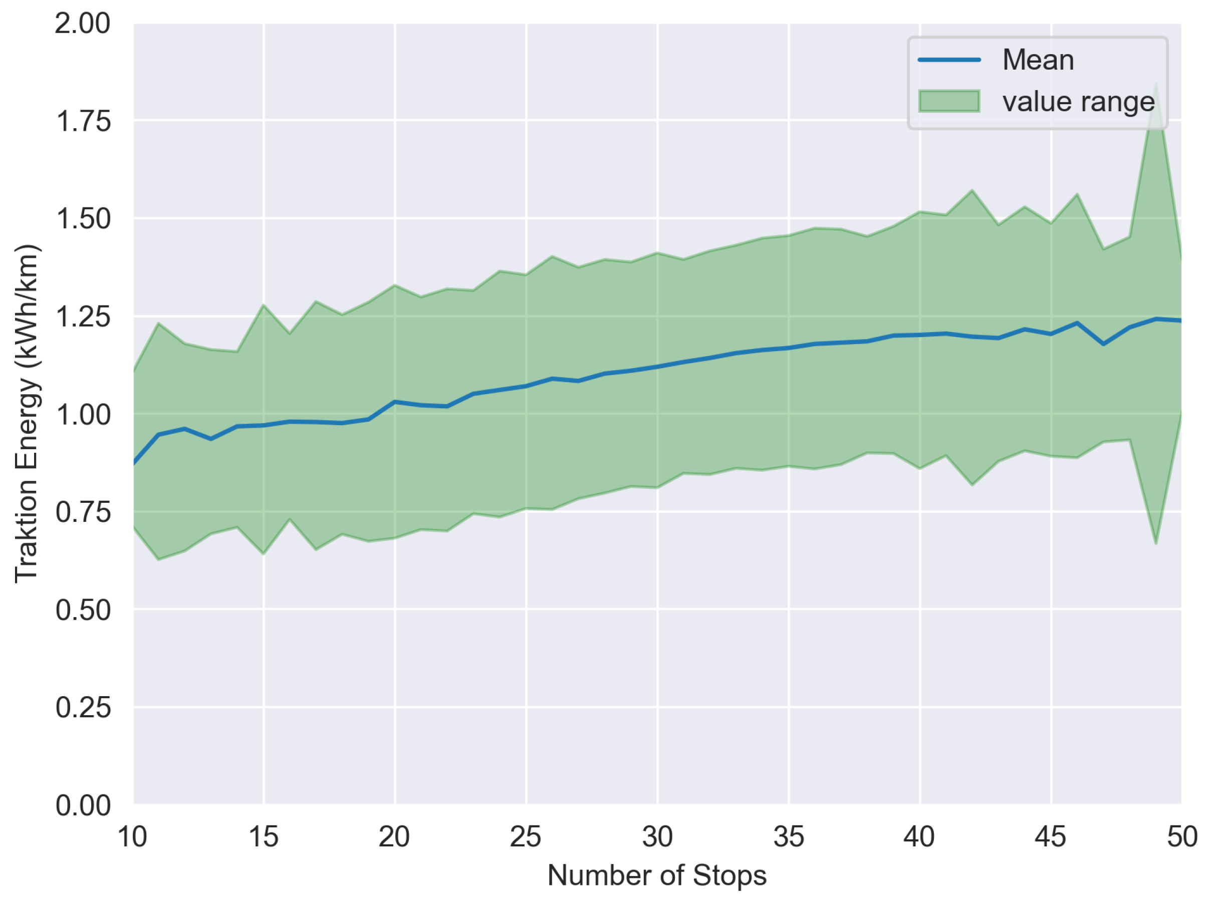
3.3.4. Traffic and Driver
4. Methodology
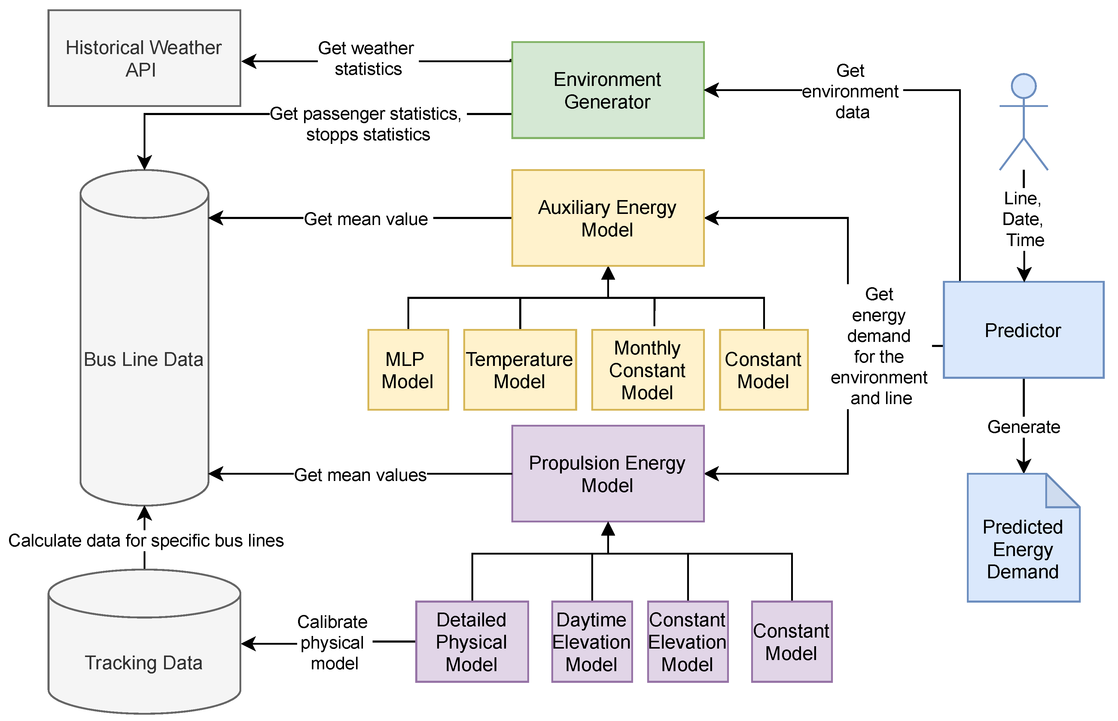
4.1. Forecasting Framework
- blue: The actor side, which includes the person using the framework; the front end of the framework, called the predictor; and the results report;
- gray: The input for the whole framework, which consists of the aggregated line data from the buses; the raw tracking data; and the historical weather data;
- purple: The propulsion energy model, which is one of the available instances (Physical Model, Daytime Altitude Model, Constant Altitude Model, or Constant Model);
- yellow: The auxiliary energy model, which is one of the available instances (MLP Model, Temperature Model, Monthly Constant Model, or Constant Model);
- green: The environment generator.
4.2. Propulsion Model
4.2.1. Constant Model
4.2.2. Constant Model with Elevation Gain
4.2.3. Daytime Model with Elevation Gain
4.2.4. Physical Model
4.3. Auxiliary Model
4.3.1. Constant Model
4.3.2. Monthly Model
4.3.3. Temperature-Based Model
4.3.4. Neural Network Model
4.4. Environment Generator
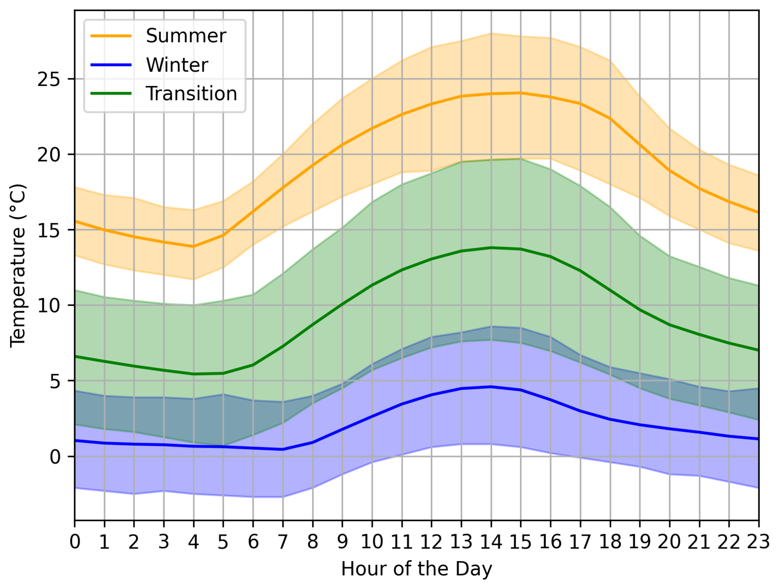
4.4.1. Weather
4.4.2. Traffic
4.4.3. Passengers
5. Results and Discussion
5.1. Model Performance and Validation of the Framework
5.2. Implications for Electric Bus Fleet Management and Optimization
5.2.1. Scenario 1: Depot Charging
5.2.2. Scenario 2: Lunch-Time Charging
6. Conclusions
- Can data-driven approaches improve energy forecasting for battery electric buses over constant value assumption for practical applications?Yes, our research clearly demonstrates that data-driven approaches markedly improve energy forecasting for BEBs. The incorporation of real-time data, such as altitude, temperature, and passenger load, into our models significantly enhances the accuracy of predictions compared to traditional constant value assumptions. This improvement is crucial for operational efficiency and strategic planning in practical applications.
- How big is the error margin for data-driven models versus constant values?The error margin for data-driven models is substantially lower than that for models based on constant values. In our study, the MAPE for data-driven models was significantly lower. For the propulsion models, the MAPE was reduced from 46.7% for the constant model to 12.9% for the daytime model. For the auxiliary models, the MAPE was reduced from 39.5% for the constant model to 25.4% for the MLP model. This reduction in the error margin underlines the efficacy of data-driven approaches in capturing the complex dynamics of BEB energy consumption.
- How can bus operators benefit from more precise energy forecasting?Bus operators stand to gain considerably from more precise energy forecasting. Firstly, it allows for more efficient route and charging schedule planning. Secondly, it can lead to cost savings by reducing the need for large batteries. Finally, accurate forecasting supports the broader objective of sustainable urban transit by facilitating the effective integration and operation of BEBs in public transport networks.
Author Contributions
Funding
Data Availability Statement
Conflicts of Interest
Abbreviations
| ANN | Artificial Neural Network |
| API | Application Programming Interface |
| BEB | Battery Electric Bus |
| EG | Environment Generator |
| GPS | Global Positioning System |
| HVAC | Heating Ventilation Air Conditioning |
| IQR | Inter Quartile Range |
| kW | Kilowatt |
| kWh | Kilowatt Hours |
| MAE | Mean Absolute Error |
| MAPE | Mean Absolute Percentage Error |
| MLP | Multilayer Perceptron |
| NN | Neural Network |
| OEM | Original Equipment Manufacturer |
| pkm | Passenger Kilometers |
| POI | Point of Interest |
| RMSE | Root Mean Squared Error |
| SOC | State of Charge |
References
- Richard Nunno. Fact Sheet|Battery Electric Buses: Benefits Outweigh Costs. 2018. Available online: https://www.eesi.org/papers/view/fact-sheet-electric-buses-benefits-outweigh-costs (accessed on 10 December 2023).
- Åslund, V.; Pettersson-Löfstedt, F. Rationales for transitioning to electric buses in Swedish public transport. Res. Transp. Econ. 2023, 100, 101308. [Google Scholar] [CrossRef]
- Borén, S. Electric buses’ sustainability effects, noise, energy use, and costs. Int. J. Sustain. Transp. 2020, 14, 956–971. [Google Scholar] [CrossRef]
- Würtz, S.; Bogenberger, K.; Göhner, U. Big Data and Discrete Optimization for Electric Urban Bus Operations. Transp. Res. Rec. 2022, 2677, 389–401. [Google Scholar] [CrossRef]
- Chao, Z.; Xiaohong, C. Optimizing Battery Electric Bus Transit Vehicle Scheduling with Battery Exchanging: Model and Case Study. Procedia Soc. Behav. Sci. 2013, 96, 2725–2736. [Google Scholar] [CrossRef]
- Xing, Y.; Fu, Q.; Li, Y.; Chu, H.; Niu, E. Optimal Model of Electric Bus Scheduling Based on Energy Consumption and Battery Loss. Sustainability 2023, 15, 9640. [Google Scholar] [CrossRef]
- Würtz, S.; Niels, T.; Bogenberger, K.; Göhner, U. Impact of Inductive Charging Infrastructure at Intersections on Battery Electric Bus Operations. In Proceedings of the ITSC 2023, 2023 IEEE Intelligent Transportation Systems Conference Proceedings, Bilbao, Spain, 24–28 September 2023. [Google Scholar]
- Bi, Z.; Keoleian, G.A.; Ersal, T. Wireless charger deployment for an electric bus network: A multi-objective life cycle optimization. Appl. Energy 2018, 225, 1090–1101. [Google Scholar] [CrossRef]
- Ko, Y.D.; Jang, Y.J. The optimal system design of the online electric vehicle utilizing wireless power transmission technology. IEEE Trans. Intell. Transp. Syst. 2013, 14, 1255–1265. [Google Scholar] [CrossRef]
- Automotiveworld.com. Efficient over Mountain and Valley: All-Electric Man Lion’s City 10 E Masters Field Test in the Dolomites. 2023. Available online: https://www.automotiveworld.com/news-releases/efficient-over-mountain-and-valley-all-electric-man-lions-city-10-e-masters-field-test-in-the-dolomites/ (accessed on 10 December 2023).
- Meishner, F.; Uwe Sauer, D. Technical and economic comparison of different electric bus concepts based on actual demonstrations in European cities. IET Electr. Syst. Transp. 2020, 10, 144–153. [Google Scholar] [CrossRef]
- Krivevski, B. Scania Unveils New Battery-Electric Bus Platform at Busworld. 2023. Available online: https://electriccarsreport.com/2023/10/scania-unveils-new-battery-electric-bus-platform-at-busworld (accessed on 10 December 2023).
- Sustainable-Bus. The Electric Bus Market in the First Half of 2023. 2023. Available online: https://www.sustainable-bus.com/news/solaris-man-byd-adl-heres-the-podium-of-the-european-electric-bus-market-for-the-first-half-of-2023 (accessed on 10 December 2023).
- Stiffler, L. The Wheels on the Bus are Battery Powered as E-Bus Use Expands. 2023. Available online: https://www.geekwire.com/2023/the-wheels-on-the-bus-are-battery-powered-as-e-bus-use-surges-ahead (accessed on 10 December 2023).
- Sustainable-Bus. 66 Per Cent Growth for US Electric Bus Market in 2022. 2023. Available online: https://www.sustainable-bus.com/news/usa-electric-bus-market-2022-calstart (accessed on 10 December 2023).
- Siöström, T. Scania Launches New Battery-Electric Bus Platform at Busworld. 2023. Available online: https://www.prnewswire.com/news-releases/scania-launches-new-battery-electric-bus-platform-at-busworld-301949308.html (accessed on 10 December 2023).
- Sustainable-Bus. 138K Electric Buses Sold in China in 2022. 2023. Available online: https://www.sustainable-bus.com/news/china-electric-bus-market-2022-subsidies/ (accessed on 10 December 2023).
- Wood, L. China $35 Billion Electric Bus Markets, Competition, Forecasts. 2023. Available online: https://finance.yahoo.com/news/china-35-billion-electric-bus-233000818.html (accessed on 10 December 2023).
- Chen, P. China Launches Pilot Program to Electrify Vehicles in Public Sector. 2023. Available online: https://www.digitimes.com/news/a20230206VL203/battery-china.html (accessed on 10 December 2023).
- JordanTimes. China’s Electric Bus Revolution Glides on. 2023. Available online: https://www.jordantimes.com/news/business/chinas-electric-bus-revolution-glides (accessed on 10 December 2023).
- Transition-China. Research on Technical Systems of Battery Electric Buses in China. 2023. Available online: https://transition-china.org/mobilityposts/research-on-technical-systems-of-battery-electric-buses-in-china/ (accessed on 10 December 2023).
- Beckers, C.J.; Besselink, I.J.; Nijmeijer, H. The State-of-the-Art of Battery Electric City Buses. In Proceedings of the 34th International Electric Vehicle Symposium and Exhibition (EVS34), Nanjing, China, 25–28 June 2021. [Google Scholar]
- Califoria Air Resources Board. Battery Electric Truck and Bus Energy Efficiency Compared to Conventional Diesel Vehicles. 2018. Available online: https://ww2.arb.ca.gov/resources/documents/battery-electric-truck-and-bus-energy-efficiency-compared-conventional-diesel (accessed on 10 December 2023).
- Misanovic, S.; Glisovic, J.; Blagojevic, I.; Taranovic, D. Influencing factors on electricity consumption of electric bus in real operating conditions. Therm. Sci. 2023, 27, 767–784. [Google Scholar] [CrossRef]
- Clarke, K.; Danoczi, J.; Fraser, R.; Jansen, R. Saskatoon Electric Bus Performance Report—January 2022. 2022. Available online: https://pub-saskatoon.escribemeetings.com/filestream.ashx?DocumentId=157285 (accessed on 10 December 2023).
- Eufrásio, A.B.R.; Daniel, J.; Delgado, O. Operational Analysis of Battery Electric Buses in São Paulo; The International Council on Clean Transportation: Washington, DC, USA, 2023. [Google Scholar]
- Čulík, K.; Štefancová, V.; Hrudkay, K.; Morgoš, J. Interior Heating and Its Influence on Electric Bus Consumption. Energies 2021, 14, 8346. [Google Scholar] [CrossRef]
- Hao, X.; Wang, H.; Lin, Z.; Ouyang, M. Seasonal effects on electric vehicle energy consumption and driving range: A case study on personal, taxi, and ridesharing vehicles. J. Clean. Prod. 2020, 249, 119403. [Google Scholar] [CrossRef]
- Martin, B.; Spiess, D.; Würtz, S.; Göhner, U.; Rupp, A. Case Study on the Impact of the Road Gradient, Passenger Loading and Recuperation Power Limitations on the Energy Consumption of Battery Electric Busese. In Proceedings of the 2023 IEEE Vehicle Power and Propulsion Conference (VPPC), Milan, Italy, 24–27 October 2023. [Google Scholar]
- Fernandes, H.J.d.S. Electric Bus Performance Evaluation in Real World Use Conditions; Universidade de Lisboa: Lisbon, Portugal, 2018. [Google Scholar]
- Vehviläinen, M.; Lavikka, R.; Rantala, S.; Paakkinen, M.; Laurila, J.; Vainio, T. Setting Up and Operating Electric City Buses in Harsh Winter Conditions. Appl. Sci. 2022, 12, 2762. [Google Scholar] [CrossRef]
- Wang, S.; Lu, C.; Liu, C.; Zhou, Y.; Bi, J.; Zhao, X. Understanding the Energy Consumption of Battery Electric Buses in Urban Public Transport Systems. Sustainability 2020, 12, 10007. [Google Scholar] [CrossRef]
- de Wilde, R. Influence of Temperature on Consumption of Battery Electric Buses and Consolidation of a Prediction Model; Ecole Polytechnique de Louvain: Ottignies-Louvain-la-Neuve, Belgium, 2022. [Google Scholar]
- Zhou, B.; Wu, Y.; Zhou, B.; Wang, R.; Ke, W.; Zhang, S.; Hao, J. Real-world performance of battery electric buses and their life-cycle benefits with respect to energy consumption and carbon dioxide emissions. Energy 2016, 96, 603–613. [Google Scholar] [CrossRef]
- Gao, Z.; Lin, Z.; LaClair, T.J.; Liu, C.; Li, J.M.; Birky, A.K.; Ward, J. Battery capacity and recharging needs for electric buses in city transit service. Energy 2017, 122, 588–600. [Google Scholar] [CrossRef]
- Würtz, S.; Spiess, D.; Martin, B.; Bogenberger, K.; Göhner, U.; Rupp, A. Energy Prediction Model Development and Parameter Estimation for Urban Battery Electric Buses with Real World Data. In Proceedings of the TRB Annual Meeting 2023, Washington, DC, USA, 8–12 January 2023. [Google Scholar]
- Beckers, C.J.J. Energy Consumption Prediction for Electric City Buses: Using Physics-Based Principles. Ph.D. Thesis, 1 (research tu/e / graduation tu/e), mechanical engineering. Technische Universiteit Eindhoven, Eindhoven, The Netherlands, 2022. [Google Scholar] [CrossRef]
- Zhou, X.; An, K.; Ma, W. Data-Driven Approach for Estimating Energy Consumption of Electric Buses under On-Road Operation Conditions. J. Transp. Eng. Part A Syst. 2023, 149, 9. [Google Scholar] [CrossRef]
- Ji, J.; Bie, Y.; Zeng, Z.; Wang, L. Trip energy consumption estimation for electric buses. Commun. Transp. Res. 2022, 2, 100069. [Google Scholar] [CrossRef]
- Chen, Y.; Wu, G.; Sun, R.; Dubey, A.; Laszka, A.; Pugliese, P. A Review and Outlook on Energy Consumption Estimation Models for Electric Vehicles. SAE J. STEEP 2021, 2, 79–96. [Google Scholar] [CrossRef]
- Lim, L.K.; Muis, Z.A.; Ho, W.S.; Hashim, H.; Bong, C.P.C. Review of the energy forecasting and scheduling model for electric buses. Energy 2023, 263, 125773. [Google Scholar] [CrossRef]
- Hjelkrem, O.A.; Lervåg, K.Y.; Babri, S.; Lu, C.; Södersten, C.J. A battery electric bus energy consumption model for strategic purposes: Validation of a proposed model structure with data from bus fleets in China and Norway. Transp. Res. Part D Transp. Environ. 2021, 94, 102804. [Google Scholar] [CrossRef]
- Li, X.; Wang, T.; Li, J.; Tian, Y.; Tian, J. Energy Consumption Estimation for Electric Buses Based on a Physical and Data-Driven Fusion Model. Energies 2022, 15, 4160. [Google Scholar] [CrossRef]
- Basma, H.; Mansour, C.; Haddad, M.; Nemer, M.; Stabat, P. Comprehensive energy modeling methodology for battery electric buses. Energy 2020, 207, 118241. [Google Scholar] [CrossRef]
- Saadon Al-Ogaili, A.; Ramasamy, A.; Juhana Tengku Hashim, T.; Al-Masri, A.N.; Hoon, Y.; Neamah Jebur, M.; Verayiah, R.; Marsadek, M. Estimation of the energy consumption of battery driven electric buses by integrating digital elevation and longitudinal dynamic models: Malaysia as a case study. Appl. Energy 2020, 280, 115873. [Google Scholar] [CrossRef]
- Pamuła, T.; Pamuła, W. Estimation of the Energy Consumption of Battery Electric Buses for Public Transport Networks Using Real-World Data and Deep Learning. Energies 2020, 13, 2340. [Google Scholar] [CrossRef]
- Pamuła, T.; Pamuła, D. Prediction of Electric Buses Energy Consumption from Trip Parameters Using Deep Learning. Energies 2022, 15, 1747. [Google Scholar] [CrossRef]
- Al-Ogaili, A.S.; Al-Shetwi, A.Q.; Al-Masri, H.M.K.; Babu, T.S.; Hoon, Y.; Alzaareer, K.; Babu, N.V.P. Review of the Estimation Methods of Energy Consumption for Battery Electric Buses. Energies 2021, 14, 7578. [Google Scholar] [CrossRef]
- Würtz, S.; Rossa, J.; Bogenberger, K.; Göhner, U. Virtual testbed for the planning of urban battery electric buses. In Proceedings of the 10th International Symposium on Transportation Data & Modelling (ISTDM2023), Ispra, Italy, 19–22 June 2023; booklet of abstracts. Volume 10, pp. 163–166. [Google Scholar] [CrossRef]
- Kammuang-lue, N.; Boonjun, J. Energy consumption of battery electric bus simulated from international driving cycles compared to real-world driving cycle in Chiang Mai. Energy Rep. 2021, 7, 344–349. [Google Scholar] [CrossRef]
- Gallet, M.; Massier, T.; Hamacher, T. Estimation of the energy demand of electric buses based on real-world data for large-scale public transport networks. Appl. Energy 2018, 230, 344–356. [Google Scholar] [CrossRef]
- Wu, X.; Du, J.; Hu, C.; Jiang, T. The influence factor analysis of energy consumption on all electric range of electric city bus in China. In Proceedings of the 2013 World Electric Vehicle Symposium and Exhibition (EVS27), Barcelona, Spain, 17–20 November 2013; pp. 1–6. [Google Scholar] [CrossRef]
- Abdelaty, H.; Mohamed, M. A Prediction Model for Battery Electric Bus Energy Consumption in Transit. Energies 2021, 14, 2824. [Google Scholar] [CrossRef]
- Lajunen, A.; Kivekaes, K.; Baldi, F.; Vepsaelaeinen, J.; Tammi, K. Different Approaches to Improve Energy Consumption of Battery Electric Buses. In Proceedings of the 2018 IEEE Vehicle Power and Propulsion Conference (VPPC), Chicago, IL, USA, 27–30 August 2018; IEEE: Piscataway, NJ, USA, 2018; pp. 1–6. [Google Scholar] [CrossRef]
- Budiono, H.D.S.; Heryana, G.; Adhitya, M.; Sumarsono, D.A.; Nazaruddin, N.; Siregar, R.; Rijanto, E.; Aprianto, B.D. Power Requirement and Cost Analysis of Electric Bus using Simulation Method with RCAVe-EV1 Software and GPS Data; A Case Study of Greater Jakarta. Int. J. Technol. 2022, 13, 793. [Google Scholar] [CrossRef]
- Kivekas, K.; Vepsalainen, J.; Tammi, K. Stochastic Driving Cycle Synthesis for Analyzing the Energy Consumption of a Battery Electric Bus. IEEE Access 2018, 6, 55586–55598. [Google Scholar] [CrossRef]
- Phyo, L.Y.; Depaiwa, N.; Yamakita, M.; Kerdsup, B.; Masomtob, M. Impact of Driving Behavior on Power Consumption of Electric Bus: A Case Study on Rama IX Bridge. In Proceedings of the 2022 International Electrical Engineering Congress (iEECON), Khon Kaen, Thailand, 9–11 March 2022; pp. 1–4. [Google Scholar] [CrossRef]
- Blades, L.A.W.; MacNeill, R.; Zhang, Y.; Cunningham, G.; Early, J. Determining the Distribution of Battery Electric and Fuel Cell Electric Buses in a Metropolitan Public Transport Network; SAE Technical Paper 2022-01-0675; SAE International: Warrendale, PA, USA, 2022. [Google Scholar] [CrossRef]
- Erkkilä, K.; Nylund, N.O.; Pellikka, A.P.; Kallio, M.; Kallonen, S.; Ojamo, S.; Ruotsalainen, S.; Pietikäinen, O.; Lajunen, A. Ebus-electric Bus Test Platform in Finland. In Proceedings of the 27th International Electric Vehicle Symposium & Exhibition (EVS27), Barcelona, Spain, 17–20 November 2013. [Google Scholar]
- Gruppe, M.N. Grundlagen der Nutzfahrzeugtechnik: Basiswissen Lkw und Bus; Kirschbaum Verlag: Bonn, Germany, 2008. [Google Scholar]
- Bartłomiejczyk, M.; Kołacz, R. The reduction of auxiliaries power demand: The challenge for electromobility in public transportation. J. Clean. Prod. 2020, 252, 119776. [Google Scholar] [CrossRef]
- Blumer, A.; Ehrenfeucht, A.; Haussler, D.; Warmuth, M.K. Occam’s Razor. Inf. Process. Lett. 1987, 24, 377–380. [Google Scholar] [CrossRef]
- Dembski, F.; Wössner, U.; Letzgus, M.; Ruddat, M.; Yamu, C. Urban Digital Twins for Smart Cities and Citizens: The Case Study of Herrenberg, Germany. Sustainability 2020, 12, 2307. [Google Scholar] [CrossRef]
- Schrotter, G.; Hürzeler, C. The Digital Twin of the City of Zurich for Urban Planning. Photogramm. Fernerkund. Geoinf. (PFG) 2020, 88, 99–112. [Google Scholar] [CrossRef]
- Hämäläinen, M. Urban development with dynamic digital twins in Helsinki city. IET Smart Cities 2021, 3, 201–210. [Google Scholar] [CrossRef]
- Statista. Battery Price Per Kwh 2023|Statista. Available online: https://www.statista.com/statistics/883118/global-lithium-ion-battery-pack-costs/ (accessed on 14 December 2023).


| Hyperparameter | Values |
|---|---|
| Learning Rate | … 0.0029 … |
| Layers | [64, 32], [64, 32, 16], [64, 32, 16, 8], [64, 32, 16, 8, 4], |
| [64, 64, 64], [2, 2, 2, 2], [8, 8, 8, 8] | |
| Activation Function | relu, tanh, sigmoid |
| Optimizer | adam, sgd, rmsprop, adadelta, adagrad, adamax |
| Loss Function | mse, mae |
| Epochs | 1000 |
| Batch Size | 16, 32, 64, 128 |
| Model | Advantages | Disadvantages |
|---|---|---|
| Auxiliary Models | ||
| Constant Model (CM) | Easy implementation | Low accuracy |
| Monthly Model | Easy implementation, | Region specific |
| better seasonal accuracy | ||
| Temperature Model | Adaptable to different cities, | Specific to vehicle types, requires |
| seasons, and climatic regions | data collection for new vehicles | |
| Neural Network | High accuracy | Requires extensive data, |
| vehicle specific | ||
| Propulsion Models | ||
| Constant Model (CM) | Easy implementation | Low accuracy |
| CM with Altitude (wA) | Accounts for topology | Requires topology data, |
| improved but still low accuracy | ||
| Daytime Model wA | Considers topology and | Location and vehicle specific |
| traffic | ||
| Physical Model | High accuracy, | Data and calibration intensive, |
| adaptable to new vehicles | requires trajectory data, | |
| and regions | e.g., from simulations | |
| Model | MAE (All Data) | MAPE |
|---|---|---|
| Constant Model | 0.524 kWh/km | 46.7% |
| Constant Model + Altitude | 0.148 kWh/km | 13.2% |
| Daytime Model + Altitude | 0.145 kWh/km | 12.9% |
| Physical Energy Model with tracking data * | 0.062 kWh/km | 5.5% |
| Model | MAE (All Data) | MAPE | MAE (Below 10 °C) | MAPE |
|---|---|---|---|---|
| Constant Model | 0.243 kWh/km | 42.6% | 0.225 kWh/km | 39.5% |
| Monthly Constant | 0.223 kWh/km | 39.1% | 0.157 kWh/km | 27.5% |
| Temperature Model | 0.222 kWh/km | 38.9% | 0.146 kWh/km | 25.6% |
| MLP Model | 0.223 kWh/km | 39.1% | 0.145 kWh/km | 25.4% |
| MLP with tracking data * | 0.091 kWh/km | 16.0% | 0.0725 kWh/km | 12.7% |
Disclaimer/Publisher’s Note: The statements, opinions and data contained in all publications are solely those of the individual author(s) and contributor(s) and not of MDPI and/or the editor(s). MDPI and/or the editor(s) disclaim responsibility for any injury to people or property resulting from any ideas, methods, instructions or products referred to in the content. |
© 2024 by the authors. Licensee MDPI, Basel, Switzerland. This article is an open access article distributed under the terms and conditions of the Creative Commons Attribution (CC BY) license (https://creativecommons.org/licenses/by/4.0/).
Share and Cite
Würtz, S.; Bogenberger, K.; Göhner, U.; Rupp, A. Towards Efficient Battery Electric Bus Operations: A Novel Energy Forecasting Framework. World Electr. Veh. J. 2024, 15, 27. https://doi.org/10.3390/wevj15010027
Würtz S, Bogenberger K, Göhner U, Rupp A. Towards Efficient Battery Electric Bus Operations: A Novel Energy Forecasting Framework. World Electric Vehicle Journal. 2024; 15(1):27. https://doi.org/10.3390/wevj15010027
Chicago/Turabian StyleWürtz, Samuel, Klaus Bogenberger, Ulrich Göhner, and Andreas Rupp. 2024. "Towards Efficient Battery Electric Bus Operations: A Novel Energy Forecasting Framework" World Electric Vehicle Journal 15, no. 1: 27. https://doi.org/10.3390/wevj15010027
APA StyleWürtz, S., Bogenberger, K., Göhner, U., & Rupp, A. (2024). Towards Efficient Battery Electric Bus Operations: A Novel Energy Forecasting Framework. World Electric Vehicle Journal, 15(1), 27. https://doi.org/10.3390/wevj15010027