An Assessment of Low-Cost Tractor Motorization with Main Farming Implements

Abstract

The objective of the present work is to evaluate the performance of a low-cost tractor equipped with a parallel hybrid engine, which was simulated using AMESim software. The tractor was evaluated with three different farming implements attached to the tractor, and each implement requires a different type of power. The first simulation was executed without any implements attached. The tractor was able to run for 170 s with the electric motor only, which resulted in fuel savings during this period. The first implement, a moldboard plow, was attached for the second round of evaluation, and the electric motor ran by itself for 150 s, which also led to fuel savings during operation. During the third simulation, the tractor was attached to a Bette Harvest, which has a very high-power demand. The obtained results show that both engines were engaged to provide the required energy. During the final round of evaluation, simulations were run for a straw tub grinder. In this simulation, the electric motor ran alone until the battery was fully discharged. Thereafter, the combustion engine was activated in order to facilitate operations and to charge the battery. The results show that the parallel hybrid architecture employed for the low-cost tractor significantly decreased the CO₂ emissions and minimized the consumption of fuel.

1. Introduction

The continuing increase in the global population requires an adequate increase in crop production to accommodate it [1]. Moreover, as the population grows, global meat consumption and the demand for bioenergy and raw materials are projected to increase [2,3]. Farm mechanization is particularly essential towards providing increased crop production, now and probably even more so in the future [4]. In addition, agricultural mechanization is generally a necessary first step in the general mechanization of a nation so that it can shift from poverty to security and prosperity. Tractors represent the largest segment of the agricultural machinery industry and play a central role in the mechanization of agriculture [5]. Global annual tractor sales are estimated at approximately 1.8 million units, with a sales volume of USD 45 billion in 2017 [6].

The Traction farming tasks is predominantly carried out by tractors with the several power [7]. The efficiency of a tractor is measured by the amount of work performed versus the cost of this work. Hitching work is affected by the traction and travel speed of the tractor used [5,8].

Because of the energy density of diesel fuel, it is commonly assumed that diesel engines will be predominantly used in the agricultural sector in the coming decades [9,10]. However, the U.S. Environmental Protection Agency (EPA) estimates that if off-road vehicle emissions are not controlled, then these vehicles will contribute 33% of hydrocarbon (HC) emissions, 9% of carbon monoxide (CO), 9% of nitrogen oxides (NOx), and 2% of particulate matter (PM) emissions in the United States over the coming years [11].

The automotive industry has already started to move towards the construction of green, environmentally friendly vehicles. This approach focuses mainly on the three areas: emissions, noise, and fuel consumption. This strategy aims to significantly reduce vehicle emissions and increase the fuel economy of vehicles, both of which are beneficial for the environment [12].

From this point of view, tractor hybridization is a valid mechanism to ensure that the environment has a cleaner future and that the costs of the agricultural industry are minimized, as scientifically demonstrated in a previous work [13].

In the present work, the behavior of a hybrid powertrain of a low-cost tractor was evaluated using the AMESim simulation tool with a moldboard plow, Bette Harvest, or straw tub grinder attached to it.

2. State of the Art

Hybrid technology is an advanced technology for improving fuel efficiency in the automotive industry. It has improved fuel efficiency in automobiles by 25% and has also contributed to improving the fuel efficiency of construction machinery [14].

In order to improve construction machinery, Komatsu developed a model (HB205) using hybrid technology based on excavator rotation that requires high power, which has reduced fuel consumption by 25% compared with its non-hybrid model [15]. Caterpillar also developed a hybrid bulldozer (D7E Hybrid) and increased fuel efficiency by 20 percent compared with its predecessor [16]. In contrast to the automotive industry, the construction machinery industry has applied hybrid technologies to workpieces such as boom and bucket systems, and most studies have focused on using excavators [17].

In particular, various studies on hydraulic pressure control strategies for motor operating parts have been carried out to improve work efficiency. For example, Wang and Wang (2014) developed a pressure compensation system to improve the energy efficiency of a hybrid hydraulic system and performed an evaluation using a bench test. They reported that 26–33% of the energy that would have otherwise been used by this system was recovered [18]. Shen, Jiang, Su, and Karimi (2015) proposed optimal control of the variable trajectory of hybrid excavators to reduce the fuel consumption of off-road vehicles, and Lin, Wang, Hu, and Gong (2010) improved the efficiency of hybrid excavators by 17% through the development and simulation of energy regeneration systems [19,20].

Choi, Kim, Yu, and Yi (2011) developed an optimal control system for hybrid excavators.

Additionally, Yoon, Truong, and Ahn (2013) developed a parallel hybrid excavator by applying an electro-hydraulic actuator, which reduced the energy usage of the machine by 60% [21,22].

In other studies, hybrid technologies have been applied to the driving components of construction machines. Zeng, Yang, Peng, Zhang, and Wang (2014) applied several energy management strategies for wheel loaders and obtained significant increases in fuel efficiency through optimal control of the power drive [23]. Hui and Jungqing (2010) developed a parallel hybrid hydraulic system to reduce energy consumption during frequent wheel loader stop/start phases and demonstrated improved work efficiency and fuel savings through simulations [24]. Dagci, Peng, and Grizzle (2015) applied a hybrid power distribution system with two single planetary gears (SPGs) in light-duty trucks, and Keulen, Mullem, Jager, Kessels, and Steinbuch (2012) proposed an optimal control strategy that was adaptable to different truck masses and road elevations and applied hybrid technology to heavy-duty trucks [25,26].

In the agricultural machinery industry, John Deere has developed a mild hybrid tractor (Model 7030E) that operates the engine compressor cooling and air conditioning systems with one engine, which has significantly increased fuel efficiency. The efficient use of power in the drive section is important because tractors require high traction force when operating with towing implements and performing soil loading; however, there have been no studies on the use of hybrid technologies in the drive section. Thus, this study was conducted to develop a hybrid tractor. The objectives of this study were (1) to build a parallel hybrid tractor using components of a hybrid drive system, (2) to establish power management strategies for the hybrid tractor, and (3) to evaluate the performance of the hybrid tractor by comparison with a conventional tractor through field testing [27].

3. Hybrid Architecture Adopted

The parallel hybrid architecture used in this study, which is shown in Figure 1, consists of a direct mechanical connection between the hybrid power unit and the wheels. It is equipped with an electric traction motor that drives the wheels and can recover some of the braking energy to charge the batteries (regenerative braking) or to assist the internal combustion engine during acceleration.

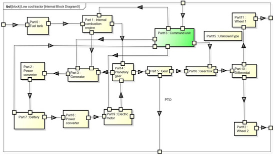
Figure 1. Principle of parallel architecture.

Furthermore, the internal combustion engine and the electric motor are coupled by a mechanical device.

The electric motor can then be designed with reduced capacity, i.e., lower cost and volume.

There are several configurations of the mechanical device used for the combination, depending on the structure between the internal combustion engine and the electric motor. There can be a coupling with a single- or two-shaft configuration, speed coupling with a planetary gearbox, or a fusion of the two [28,29].

The appropriate operating mode is programmed or manually switched on [13]:

• At high speeds, the combustion engine is used as the drive.
• At low speeds, the electric motor is activated to optimize fuel efficiency and consumption; the electric motor does not run at a standstill to save the battery.
• When the driver strongly accelerates, both the electric and combustion engines work simultaneously to transmit more power.

When the driver lifts his or her foot while driving or braking, the electric motor works as a generator and recovers energy. The combustion engine is then decoupled from the transmission and thus, generates few losses.

The low-cost tractor is an agricultural tractor that weighs 4.5 t and is equipped with a four-stroke V8 combustion engine with a total displacement of 12 L and a power of 120 kW. The appropriate selection of the electric part of the hybrid vehicle is a major element of the successful marriage between the thermal and electric engines. The permanent magnet synchronous motor (MSAP) appears to be an optimal solution for automotive traction because of its technical performance and, in particular, its compactness and efficiency. This type of motor is used by Toyota in the Prius for its high efficiency and good dynamic performance, which is attributed to the low stator inductances due to the large width of the apparent air gap, large magnetic field in the air gap, and lack of a DC voltage source for excitation. The low-cost tractor in this study is equipped with 20 kW synchronous motors. The outputs of the two engines are linked by a planetary gear train. The output power is adapted by a manual gearbox with four gears. In addition, it is equipped with a generator that can recover the electric energy from the combustion engine and store it in a lithium battery.

4. Mathematical Model

In the present work, we examined a model of a parallel hybrid tractor using AMESim software. The main notation used in this paper is shown in the Table 1. We produced the 1D sketch shown in Figure 2 and then determined the appropriate mission for each attached implement in order to evaluate the tractor’s behavior during the mission.

Table 1. Main notation used in this paper.

Symbol	Description
${\rho }_{air}$	Air density
Sx	Active area of the vehicle for air resistance
Cx	Coefficient of drag for longitudinal axis translation
Cz	Coefficient of drag for translation on the vertical axis
Wx	Stirring coefficient for the translation on the longitudinal axis
Wz	Stirring coefficient for translation on the vertical axis
$T1$	Front-wheel torque
$T2$	Rear-wheel torque
$rad1$	Front-wheel radius
$rad2$	Rear-wheel radius
$M_{car}$	Mass of the vehicle
$g$	Gravity
${\alpha }_{slope}$	Slope angle in rad
$\alpha$	Angle of slope in %
$V_{car}$	Longitudinal speed of the vehicle
$r_{vehi}$	Viscous coefficient of friction
$F_{roll}$	Rolling resistance force
$R_{roll}$	Coefficients of rolling friction
$W_z$	Vertical wind coefficient
$V_{wind}$	Wind speed
$F_{trailer}$	Resistive force from the connected tool
$M_{trail}$	Trail mass capture
$rin1$	Rear-wheel inertia
$rin2$	Front-wheel inertia
$F_{engine}$	Driving force
Braketorq	Braking torque required by the driver [Nm]
Torbrakdrv	Driver brake control [Nm]
Maxtorqveh	Maximum braking torque of the vehicle [Nm]
Sommetorq	Torque required by the driver [Nm]
Torvehdrv	Driver acceleration control [W or Nm]
tmaxMel	Maximum engine torque [Nm]
Braketorq	Braking torque required by the driver [Nm]
sensorMErev	Speed of the electric motor [rpm]
Tpull	Torque of the electric motor for lifting [Nm]
sensorME	Speed of the electric motor [rad/s]
Gearratio	Transmission ratio between the electric motor and the vehicle
torME	Torque control of the electric motor [Nm]
Gainaccel	Gain on acceleration control
tmaxMel	Maximum engine torque [Nm]
Gearatio	Transmission ratio between the electric motor and the vehicle
Torbrak	Brake control
Gainbrakes	Gain on brake control
Maxtorqveh	Maximum braking torque of the vehicle [Nm]
tminMel	Minimum engine torque
tmaxMth	Maximum engine torque [Nm]
throttleMT	Thermal engine load
Gainacce	Gain on acceleration control
Clutchsig	Clutch control
starteng	Firing: engine on/off
torME	Torque control of the electric motor [Nm]
torbrak	Brake control
maxtorqveh	Maximum braking torque of the vehicle [Nm]
sensorME	Rotational speed of the electric motor [rad/s]
gainaccel	Gain on acceleration control
${\omega }_{pa}$	Rotational speed of the driven axle
$paratio$	Drive axle transmission ratio
$ratio$	Transmission ratio of the engaged gear
$\omega p$	Speed of rotation of the input shaft
$\omega s$	Speed of rotation of the secondary shaft
$Tslip$	Maximum Coulomb friction torque
$\omega rel$	Relative rotational speed
$dvel$	Speed threshold of the rotating stick
$Ts$	Secondary shaft torque
$nu$	Efficiency of the engaged gear
$Tloss$	Loss of torque
$ratio$	The transmission ratio of the engaged gear
$paratio$	Drive axle transmission ratio
$Ts$	Torque transmitted by the secondary shaft
$vis$	Coefficient of viscous friction on the flywheel
${\omega }_p$	Flywheel rotation speed
$powerPr$	Input shaft power $\left(\mathrm{Tp}-\mathsf{\omega }\mathrm{p}\right)$
$powerPa$	Power to the drive axle $\left(\mathrm{Tpa}-\mathsf{\omega }\mathrm{pa}\right)$
$BMEP$	Average effective brake pressure $\left[\mathrm{bar}\right]$
$PMF$	Mean effective friction pressure $\left[\mathrm{bar}\right]$
$Tout$	Engine output torque $\left[\mathrm{Nm}\right]$
$Tfric$	Engine friction torque $\left[\mathrm{Nm}\right]$
$V$	Swept volume of the engine $\left[\mathrm{L}\right]$
$TmaxcetTminc$	Maximum and minimum corrected torques
$Tmax$	Maximum engine torque read from the file $\left[\mathrm{Nm}\right]$
$\rho ref$	Reference ambient air density $\left[\mathrm{kg}/\mathrm{m}3\right]$
$Tamb$	Ambient air temperature $\left[\mathrm{K}\right]$
Tref	Reference ambient temperature $\left[\mathrm{degC}\right]$
$Tmax$	Maximum engine torque [Nm]
$Tfric,Thot$	Frictional torque at high engine temperature [Nm]
$Tfric,Temp$	Frictional torque at the current temperature [Nm]
$Thot$	“Hot engine temperature” parameter [degC]
$Temp$	Current engine or oil temperature $\left[\mathrm{degC}\right]$
$contre$	Actual fuel consumption
$consfile$	Value read from the fuel file
$kstart$	Overconsumption when starting the engine
$expfcons$	Effect of cold temperature (user-defined expression)
$\phi$	Current equivalency report
$\phi file$	Value read from the data file
$expeqratio$	Effect of cold temperature (user-defined expression)
$dmexh$	Exhaust gas mass flow rate [g/s]
$cons$	Fuel consumption [g/s]
$AFsto$	Stoichiometric air/fuel ratio [null]
$w$	Motor speed [rpm]
$idlespeed$	Engine idling speed [rpm]
$flow0$	Fresh air mass flow rate at idle [g/s]
$Teng$	Motor temperature [degC]
$Thigh$	High threshold for motor temperature parameter [degC]
$Tlow$	Low threshold for motor temperature parameter [degC]
$coefcoldCO$	Correction coefficient for cold CO emission
$coefstCO$	Coefficient of CO when enriching the fuel when starting the engine
$kstart$	Overconsumption when starting the engine
$emiCOfile$	Value of CO
$FichierFMEP$	Average effective friction pressure read in the [bar] file
$expfmepcor$	Temperature effect correction (user-defined expression)
$Texhaustfile$	Exhaust gas temperature read in the [degC] file
$expexhtemp$	Temperature effect correction (user-defined expression)
$coefheatwall$	Combustion heat ratio for wall heating
$cons$	Fuel consumption [kg/s]
$pci$	Specific calorific value of the fuel [J/kg]
$exphlosses$	Correction of the effect of temperature
$cons$	Fuel consumption [kg/s]
$emiHC$	HC emissions [kg/s]
$emiCO$	CO emissions [kg/s]
$pci$	Specific calorific value of the fuel [J/kg]
$dmBG$	Burnt exhaust gas
$dmunburnedair$	Exhaust unburned air mass flow rate (when φ ≤ 1)
Unburned fuel	Exhaust unburned fuel mass flow rate (when φ ≥ 1)
$CpBG$	Thermal capacity of the flue gas set by the user [J/K/kg] for φ = 1
$Cpcarb$	Heating capacity of the fuel set by the user [J/K/kg]
$Paire$	Thermal capacity of fresh air and gas set at 1040.0 [J/K/kg]
$ncyl$	Total number of engine cylinders
$ncy{l}_{deac}$	Number of deactivated cylinders
$ncylac$	Number of activated cylinders
$BME{P}_{max}$	Maximum BMEP read from the file and corrected for temperature effects
$FMEP$	FMEP read from the file at current load and corrected for temperature effects
$FME{P}_0$	FMEP at zero load
$Tmin$ and $Tmax$	Negative and positive torque corresponding to defined parameters
$Tm$	Couple $\left[\mathrm{Nm}\right]$
$\omega$	Speed of rotation $\left[\mathrm{rad}/\mathrm{s}\right]$
$Pelec$	Electrical power $\left[\mathrm{W}\right]$
SOC	State of charge
DOD	Depth of discharge
CPVO	Open-circuit voltage
V2	Potential at negative pole [V]
fixedvoltage	Fixed battery voltage [V]
fixedcellvoltage	Fixed cell voltage [V].
Seal	Number of cells in series
CPVObat	Open-circuit voltage read from the file/expression for the whole battery [V]
OCVcell	Open-circuit voltage read from the file/expression for a cell [V]
Rbat	Internal resistance read from the file/expression for the whole drum set [Ohm]
Rcell	Internal resistance read from the file/expression for a cell [Ohm]
I3	Battery current at the positive pole [A]
Icell	Cellular current [A]
Cell	Number of cells in series
Cell	Number of parallel cells

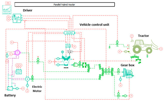
Figure 2. Sketch of the parallel hybrid tractor.

The duty cycles of agricultural tractors are very different from the cycles known to the automotive industry. The hybrid tractor operates according to the maximum speeds for each implement, as shown in Table 2 [30].

Table 2. Parameters of implements.

Implement	Name of Implement	Maximal Velocity	The Needed Force for Implements
	Moldboard plow	7 km/h	Draft power
	Bette Harvest	8 km/h	PTO + Draft power
	Straw tub grinder	0 km/h	PTO power

4.1. Definition of the Sub-Models Composing the Sketch

4.1.1. Tractor

The tractor sub-model is a 1D vehicle load sub-model and is used to calculate longitudinal acceleration. The speed and displacement are defined for a vehicle with two axles, taking into consideration the rolling friction and road gradient [31].

The acceleration is calculated based on the following forces:

Engine force:

$$F_{engine}=\frac{T1}{rad1}+\frac{T2}{rad2}$$

(1)

Slope strength [32]:

$$F_{slope}=M_{car}.g.sin\left({\alpha }_{slope}\right)$$

(2)

Rolling frictional force [33]:

$$F_{friction}=r_{vehi}.V_{car}+F_{roll}.sign\left(Vcar\right)$$

(3)

$$F_{roll}=R_{roll}\left(M_{because}.g.cos\left({\alpha }_{slope}\right)-W_z.V_c\right)$$

(4)

$$V_c = \left(V_{car} + V_{wind}\right). \left|V_{car} + V_{wind}\right|$$

(5)

Aerodynamic force [33]:

$$F_{aero}=W_x.V_c$$

(6)

according to Newton’s second law.

The sum of all forces applied to the vehicle is divided by the body mass, including wheel inertias and trailer mass, to obtain vehicle acceleration.

$$A_{car}=\frac{1}{M_{vehi}+M_{trail}+\frac{rin1}{{\left(rad1\right)}^2}+\frac{rin2}{{\left(rad2\right)}^2}}.(F_{engine}-F_{aero}-F_{slope}-F_{friction}-F_{trailer})$$

(7)

Then, this acceleration is integrated twice to obtain the speed and position of the vehicle.

4.1.2. Control Unit

The control unit receives information from the driver (acceleration, braking controls, and gearbox ratio), the electric motor (maximum/minimum speed and torque), the combustion engine (maximum speed and torque), the battery (state of charge), and the vehicle speed and the gearbox (input shaft speed). The unit analyzes these values in order to minimize battery consumption. The electric motor can be used as a generator to charge the battery when the driver brakes.

In this approach, the electric motor and the combustion engine are connected to the manual gearbox. The control unit manages the power required by the engine and the electric motor. If the battery needs to be regenerated, then the motor is used to move the vehicle forward, and if the power demand is less than its optimum power (depending on its speed), then the difference is transmitted to the electric motor/generator to charge the battery.

The strategy consists of four modes:

• Mode 1: The battery must not be charged; the combustion engine is not used.
• Mode 2: The battery does not need to be charged; the combustion engine is used.
• Mode 3: The battery is fully charged; the engine is not used.
• Mode 4: The battery is not fully charged; the engine is used.

There are two transient modes when the engine starts:

• If the engine speed is less than idle speed/2, then the clutch is engaged and the engine does not start.
• When the engine reaches idle speed/2, the clutch remains closed and the engine starts [34].

The braking torque required by the driver is calculated following the selected brake command, as defined in Table 3.

Table 3. Brake command.

	Brake Command: Signal [0.1]	Brake Command: Wheel Torque (Nm)
braketorq	$torbrakdrv\cdot maxtorqveh$	$torbrakdrv$

• Mode 1: The battery is fully charged; the combustion engine is not used.

In this mode, the electric motor is used to drive the vehicle, the combustion engine is stopped, and the clutch is opened.

The mode changes if one or both of the following conditions apply:

• The battery charge state is below the lower limit (parameter) and the engine can start (the rotation speed of the gearbox input shaft is higher than the engine idling speed).
• The vehicle speed is above the speed limit (parameter).

The torque required by the driver is calculated as defined in Table 4 and Table 5.

Table 4. Torque command.

	Sommetorq
Acceleration signal command [0.1]	$torvehdrv\cdot tmaxMel-braketorq$
Acceleration control: wheel power [W]	if |sensorMErev| < 1.0 in torvehdrv > 0 $tpull$ if |sensorMErev| < 1.0 in torvehdrv ≤ 0 $-braketorq$ if |sensorMErev| ≥ 1.0 $torvehdrv/\left|sensorME\right|/gearatio-braketorq$
Acceleration control: wheel torque [Nm]	$\frac{torvehdrv}{gearatio}-braketorq$

Table 5. Torque required.

	TorME	Torbrak
Torque requested by the driver is positive (acceleration requested)	$MIN(sommetorq.$ $gainaccel,$ $tmaxMel)$	0
Torque requested by the driver is negative or null (brake requested) and no gear is selected	0	$\left(torME.gearati-sommetorq\right).$ $\frac{gainbrakes}{maxtorqueh}$
Torque requested by the driver is negative or null (brake requested) and no gear is selected	$MAX(\frac{sommetorq}{gearation},$ $tminMel)$	$torMe.gearatiosommetorq$ $\frac{gainbrakes}{maxtorqveh}$.

• Mode 2: The battery is not fully charged; the combustion engine is used.

In this mode, the engine is used to drive the vehicle (only during acceleration), and the clutch is closed.

The mode changes if one or both of the following conditions apply:

• The battery charge status is below the lower limit (parameter).
• Vehicle speed is below the speed limit (parameter).

The torque required by the driver is calculated as defined in Table 6.

Table 6. Motor control.

	Sommetorq
Acceleration command: signal [0.1]	$Torvehdrv.tmaxMth-braketorq$
Acceleration command: wheel power [W]	Si |sensorMErev| < 5.0 and torvehdrv > 0 $tpull.gearatio$ Si |sensorMErev| < 5.0 en torvehdrv ≤ 0 $-braketorq$ Si |sensorMErev| ≥ 5.0 $torvehdrv/\left|sensorME\right|/gearatio-braketorq$
Acceleration command: wheel power [Nm]	$\frac{torvehdrv}{gearatio}*braketorq$

The motor control is calculated according to Table 7.

Table 7. Motor control.

	ThrottleMT	Clutchsig	Starteng
Torque requested by the driver is positive (acceleration requested).	$\frac{MIN\left(sommetorq.gainaccel,tmaxMth\right)}{tmaxMth}$	1	1
Torque requested by the driver is negative or null (acceleration requested).	0	0	0 or 1 function of engdecel parameter

The torque control of the electric motor and the braking control of the vehicle is calculated as shown in Table 8.

Table 8. Torque required.

	TorME	Torbrak
Torque requested by the driver is positive (acceleration requested).	0	0
Torque requested by the driver is negative or null (brake requested) and no gear is selected.	0	$$\begin{gathered} (torME.gearatio \\ -sommetorq)\frac{gainbrakes}{maxtorqueh} \end{gathered}$$
Torque requested by the driver is negative or null (brake requested) and the gear is selected.	$MAX\left(\frac{sommetorq}{gearratio},tminMel\right)$	$$\begin{gathered} (torME.gearratio \\ -sommetorq).\frac{gainbrakes}{maxtorquveh} \end{gathered}$$

• Mode 3: The battery is fully charged; the engine is not used.

In this mode, the electric motor is used to drive the vehicle, the combustion engine is stopped, and the clutch is opened. However, we account for the fact that the engine must be started to regenerate the battery.

The mode will change if one or more of the following conditions apply:

• The battery’s state of charge is above the upper limit (parameter).
• Vehicle speed is above the speed limit (parameter).
• The engine can be started (the rotation speed of the gearbox input shaft is higher than the engine idle speed).

The torque required by the driver is calculated as shown in Table 9.

Table 9. Torque required by the driver.

	Sommetorq
Acceleration command: signal [0.1]	$Torveh.tmaxMel-braketorq$
Acceleration command: wheel power [W]	if |sensorMErev| < 1.0 and torvehdrv > 0 $tpull$ if |sensorMErev| < 1.0 and torvehdrv ≤ 0 $-braketorq$ if |sensorMErev| ≥ 1.0 $torvehdrv/\left|sensorME\right|/gearatio-braketorq$
Acceleration command: wheel torque [Nm]	$\frac{torvehdrv}{gearatio}-braketorq$

The torque control of the electric motor and the braking control of the vehicle are calculated according to Table 10.

Table 10. Torque required.

	TorME	Torbrak
Torque requested by the driver is positive (acceleration requested)	$MIN(sommetorq.$ $gainaccel,tmaxMel)$	0
Torque requested by the driver is negative or null (brake requested) and no gear is selected	0	$$\begin{gathered} (torqME.gearatio \\ -sommetarq). \end{gathered}$$ $\frac{gainbrakes}{maxtorqveh}$
Torque requested by the driver is negative or null (brake requested) and no gear is selected	$MAX(\frac{sommetorq}{gearatio},$ $tminMel)$	$$\begin{gathered} (torqME.gearatio \\ -sommetarq) \end{gathered}$$ $.\frac{gainbrakes}{maxtorqveh}$

• Mode 4: The battery is not fully charged; the engine is used.

In this mode, the electric motor is used to charge the battery, and the engine is used to drive the vehicle and charge the battery (only during acceleration).

The mode changes if one or both of the following conditions apply:

• The battery’s state of charge is above the upper limit (parameter).
• The engine cannot be used (the speed of rotation of the gearbox input shaft is lower than the engine idle speed).

The torque required by the driver is calculated as shown in Table 11.

Table 11. Torque required.

	Sommetorq
Acceleration command: signal [0.1].	$Torvehdrv.$ $tmaxMth-braketorq$
Acceleration command: wheel power [W]	if |sensorMErev| < 1.0 and torvehdrv > 0 $tpull$ if |sensorMErev| < 1.0 and torvehdrv ≤ 0 $-braketorq$ if |sensorMErev| ≥ 1.0
Acceleration command: wheel torque [Nm]	$\frac{torvehdrv}{gearatio}-braketorq$

The torque control of the electric motor and the braking control of the vehicle is calculated as according to Table 12.

Table 12. Torque control.

	TorME	Torbrak
Torque requested by the driver is positive (acceleration requested) and the torque requested for the engine is lower than the optimum torque.	$MAX(sommetorq.$ $gainaccel,$ $tmiMel)$	0
Torque requested by the driver is positive (acceleration requested) and torque requested for the engine is higher than the optimum torque.	0	0
Torque requested by the driver is negative or null (brake requested) and the gear is selected.	0	$$\begin{gathered} (torqME.gearatio \\ -sommetarq).\frac{gainbrakes}{maxtorqveh} \end{gathered}$$

Engine control is calculated as defined in Table 13 [35].

Table 13. Engine control.

	Throttlemt	Clutchsig	Starteng
Torque requested by the driver is positive (acceleration requested) and the torque requested for the engine is lower than the optimum torque.	$\frac{MIN\left(sommetorq.gainaccel-torME,tmaxMth\right)}{tmaxMth}$	1
Torque requested by the driver is positive (acceleration requested) and the torque requested for the engine is higher than the optimum torque.	$\frac{MIN\left(sommetorq.gainaccel-torME,tmaxMth\right)}{tmaxMth}$	1
Torque requested by the driver is negative or null (brake requested).	0	0	1 or 1 function of engdecel parameter

4.1.3. Gearbox

This model can be used to perform simple dynamic modeling of an n-speed manual gearbox (forward and reverse). The transmission losses are the same for each gear. The inertia of the input shaft and the drive axle are taken into account.

This gearbox is composed of an input shaft, flywheel, gears, clutch/synchronizer, and drive axle [36].

The gearbox is illustrated in Figure 3.

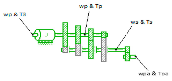
Figure 3. Operation modes of the gear of a gearbox.

• Torque loss

The torque loss set by the user must always be positive. A pre-treatment is carried out to ensure that the torque is always resistant to movement.

No further pre- or post-processing is carried out by the component.

The value read from the file is applied to the torque of the secondary shaft [37].

$$T_p\cdot ratio=-T_s+T_{loss}$$

(8)

• Input shaft speed

The input shaft speed ω_p is calculated from the motor torque at port 3, T3, and the input shaft torque, T_p (see below for the calculation of T_p).

The output rotation speed ${\omega }_3$ is determined as follows [38]:

$${\omega }_3=-{\omega }_p$$

(9)

• Rotational speed of the secondary shaft

The rotational speed of the secondary shaft ${\omega }_s$ is calculated as follows [39]:

$${\omega }_s=-{\omega }_{pa}\cdot paratio$$

(10)

• Torque transmitted by the secondary shaft

The relative speed $\left({\omega }_{rel}\right)$ between the primary and secondary shafts must first be calculated [40]:

$${\omega }_{rel}=\frac{{\omega }_p}{ratio}+{\omega }_s$$

(11)

The torque on the secondary shaft $T_s$ is the torque transmitted by the synchronizer; its calculation depends on the chosen friction model.

Hyperbolic tangent:

$$T_s=T_{slip}\cdot tanh\left(2\cdot -\frac{{\omega }_{rel}}{d_{vel}}\right)$$

(12)

• Torque transmitted by the drive shaft

The torque calculation $T_p$ of the input shaft depends on the definition of the selected speed loss [41].

$$T_p=\frac{1}{nu}\cdot \frac{-T_s}{ratio{T}_p}=\frac{-T_s+T_{loss}}{ratio}$$

• Torque transmitted by the drive axle

We assume the efficiency of the drive axle to be 1.0 (no loss).

The torque transmitted by the drive axle $T_{pa}\left(=T2\right)$ is calculated as follows [42]:

$$T_{pa}=-T_s\cdot paratio$$

(13)

• Power Losses

There are three sources of power loss: the viscous friction of the flywheel, clutch slippage, and the efficiency of the machines.

In the event of a loss of power, the power lost from the gearbox is calculated as follows [43]:

$$powerlost=vis\cdot {\omega }_p{}^2+\left|powerPr-powerPa\right|$$

(14)

4.1.4. Internal Combustion Engine

The internal combustion engine (ICE) is a sub-model with different application cases.

To apply corrections and dependencies for engine starting, cold and hot temperatures are provided and can be used.

This engine component must be used whenever information on engine performance during a cycle is required. The prediction of fuel consumption or emissions during driving cycles is accurate and has a low CPU cost (compatible with a fixed time step).

Mean effective pressures (BMEP, FMEP) and couples are related by the following relationships for a four-stroke engine [13]:

$$BMEP=4\cdot \pi \cdot Tout\cdot 0.01V$$

(15)

$$FMEP=4\cdot \pi \cdot Tfric\cdot 0.01V$$

(16)

• Torque calculation

The engine output torque is calculated from the engine control unit (ECU) load demand as follows [44]:

$$Tout=Tmaxc\cdot load+Tminc\cdot \left(1-load\right)$$

(17)

Several corrections can be activated/applied to the torque values read from the file.

These corrections are maintained simultaneously when they are all activated.

• Dynamic Correction

$$Tmaxc=Tmaxfile\cdot \frac{\rho air}{\rho ref}\cdot \sqrt{\frac{Tamb}{273.15+Tref}}$$

(18)

• Impact of temperature

If the “use temperature influence correction for FMEP” (with torque impact) option is enabled, any variation in FMEP due to a temperature that differs from the hot reference temperature will impact the engine’s torque performance.

The correction is as follows [45]:

$$Tmaxc=Tmaxfile-\Delta Tfricavec\Delta Tfric=\{\begin{array}{cc}Tfric,Temp-Tfric,& Thot\mathrm{If}\mathrm{the}\mathrm{correction}\mathrm{is}\mathrm{activated}\\ 0& \mathrm{otherwise}\end{array}$$

(19)

• Fuel consumption

The engine’s fuel consumption is read and corrected if necessary.

These corrections are maintained simultaneously when all of them are activated, and they can be applied to the value read from the:

➢

Impact of temperature;

➢

Overconsumption when starting the engine;

➢

Deactivation of cylinders.

The actual fuel consumption is calculated as follows [46]:

$$cons=consfile\cdot \left(1+kstart\right)\cdot expfcons$$

(20)

The coefficient $\mathrm{expfcons}$ is set to 1 when the temperature influence option is not activated.

• Engine Emissions
• Equivalence report

The equivalence ratio is used to determine the total exhaust mass flow rate and is calculated as follows [47]:

$$\varphi =\varphi file\cdot \left(1+kstart\right)\cdot expeqratio$$

(21)

Note: The expeqratio coefficient is set to 1 when the temperature influence option is not activated.

• Exhaust gas mass flow rate

The exhaust flow rate is calculated from the fuel consumption and the equivalence ratio, as defined in Table 14.

Table 14. Exhaust flow.

Positive Charge	Engine Brake
$dmexh=cons\cdot \left(\frac{AFsto}{\varphi }+1\right)$	$dmexh=flow0\frac{w}{idlespeed}+cons$

• Pollutant emissions

Pollutant emissions are read from related data files and corrected if necessary [48].

$$emiCO=emiCOfile\cdot \underset{\begin{array}{l}\mathrm{If}\mathrm{temperature}\\ \mathrm{influence}\mathrm{activated}\end{array}}{\underbrace{\left(\alpha t+\beta t\cdot coefcoldCO\right)}}\cdot \underset{\begin{array}{l}\mathrm{If}\mathrm{start}\mathrm{influence}\\ \mathrm{activated}\end{array}}{\underbrace{(1+kstart\cdot coefstCO)}}$$

(22)

$$\alpha t=\frac{Teng-Tlow}{Thigh-Tlow}ad\beta t=1-{\alpha }_t$$

(23)

When the engine temperature is below the “high engine temperature threshold”, a linear interpolation between the low and high temperature thresholds is performed to correct the emissions read from the user-defined data tables.

• Exhaust gas temperature

$$Texhaust=Texhaustfile\cdot expexhtemp$$

(24)

The coefficient $\mathrm{expexhtemp}$is set to 1 when the temperature influence option is not activated [49].

• Heat loss from engines

Friction mean effective pressure:

$$FMEP=FMEPfile\cdot expfmepcor$$

(25)

The coefficient $\mathrm{expfmepcor}$ is set to 1 when the temperature influence option is not activated or if the FMEP file includes an engine temperature axis.

The frictional power losses [W] are obtained from the friction torque [W]. $Tfric$ [Nm] and engine speed w [rad/s] are determined as follows [50]:

$$Pfric=Tfric\cdot \omega$$

(26)

• Losses of combustion heat

The combustion heat losses (Pcomb power [W]) are calculated using the heat loss coefficient read from the table heatwall_i.data and the quantity of fuel injected [51].

$$Pcomb=cons\cdot pci\cdot coefheatwall\cdot exphlosses$$

(27)

• Energy balance

In custom mode, it is possible to activate the energy balance function. The energy balance can be used to determine exhaust gas temperature or combustion heat losses.

The energy balance is established as follows [52]:

$$\varphi comb=Pwork+Pfric+Ppump+Pevap+Pcomb+Pexh$$

(28)

The heat of combustion $\phi comb$ [W] indicates released energy. This energy takes into account the production of CO and HC (instead of only CO₂ and H₂O for complete combustion) [53].

$$\varphi comb=\left(cons-emiHC-\frac{emiCO}{4}\right)\cdot pci$$

(29)

The fuel evaporation energy $Pevap$ [W] is deduced from the fuel consumption and the latent heat of evaporation $Hevap$ [J/kg] and is equal to [54]:

$$Pevap=cons\cdot Hevap$$

(30)

The motor output power and friction losses Pwork, Pfric [W] are equal to [55]:

$$Pwork=Tout\cdot wandPfric=Tfric\cdot w$$

(31)

The motor pumping losses (when available) $Ppump$ [W] are deduced from the value read in the pump PMEP file [bar] as follows [56]:

$$Ppump=Tpump\cdot w$$

(32)

The exhaust power of the engine $Pexh$[W] is equal to [57]:

$$\begin{gathered} Pexh=\left(dmBG\cdot CpBG+dmunburnedair\cdot Cpair+dmunburnedfuel\cdot Cpcarb\right) \\ \cdot \left(Texhaust-Tamb\right) \end{gathered}$$

(33)

• Deactivation of cylinders

The engine component receives the number of deactivated cylinder(s) at port 4 and the activation (or not) of specific corrections.

When the input signal to port 4 applies the data, correction is set to 0.0 (option 1), and no correction is applied to the supplied data file.

When the input signal to port 4 applies the data, correction is set to 1.0 (option 2), and corrections are applied to the value read from the data file.

When option 2 is selected, the corrections are as follows [58]:

$$FMEPc=FMEP\cdot \frac{ncy{l}_{ac}}{ncyl}+FME{P}_0\cdot ncyldeacncyl$$

(34)

$$BME{P}_{maxc}=BME{P}_{max}\cdot \frac{ncy{l}_{ac}}{ncyl}-FME{P}_0\cdot \frac{ncy{l}_{deac}}{ncyl}$$

(35)

Note: The minimum BMEP is not affected by cylinder deactivation.

An equivalent BMEP (BMEPeq) is calculated and used to read the data file. This is the BMEP that the engine will produce with all cylinders activated and with the same ECU load demand.

It is calculated as follows [58]:

$$BMEPeq=load\cdot \frac{1}{ncy{l}_{ac}}\cdot \left(ncyl\cdot BME{P}_{max}+ncy{l}_{deac}\cdot FME{P}_0\right)+\left(1-load\right)\cdot BME{P}_{min}$$

(36)

The engine’s fuel consumption and emission variables are also corrected if the cylinder is deactivated with option 2 selected [13].

$$cons=con{s}_{std}\cdot \frac{ncy{l}_{ac}}{ncyl}$$

(37)

$$emiCO=emiCOstd\cdot \frac{ncy{l}_{ac}}{ncyl}$$

(38)

The equivalence ratio and exhaust gas temperature variables are not affected by cylinder deactivation.

• Displacement variation

As with cylinder deactivation, the data file for combustion mode, n, with displacement variation must be completed using the BMEP calculated with the standard displacement. In this case, the standard displacement (engine parameter) is the largest available engine displacement.

The variation in the displacement vdis (≤1) is an input signal. The correction is made as follows:

$$BMEPeq=\frac{BMEPeq}{vdis}$$

(39)

The BMEPeq is used to read the data files [59].

4.1.5. Electric Motor/Generator

The following is a sub-model of an electric motor/generator with its converter. It is bi-directional (motor/generator) and independent of the technology of the motor and its converter.

• Torque

From the input torque demand $Tset$, the couple $Tlim$ is limited as follows:

$$Tmin\le Tlim\le Tmax$$

(40)

The output torque $Tm$is determined from the limited torque $Tlim$ using a first-order offset [60]:

$$Tm=11+tr\cdot s\cdot Tlim$$

(41)

where tr is the user-defined time constant [s].

• Power balance

The mechanical power $Pmec$ $\left[\mathrm{W}\right]$ is calculated as follows [61]:

$$Pmec=Tm\cdot \omega$$

(42)

The power loss $Plost\left[\mathrm{W}\right]$ is calculated from the efficiency$\eta$:

$$Plost=\left(1-\eta \right)\cdot \left|Pmec\right|$$

(43)

Two modes can then be defined:

• $Pelec>Pmec$ Motor mode.
• $Pelec<Pmec$ Generator mode.

The different modes of operation of the electric motor/generator are illustrated in Figure 4.

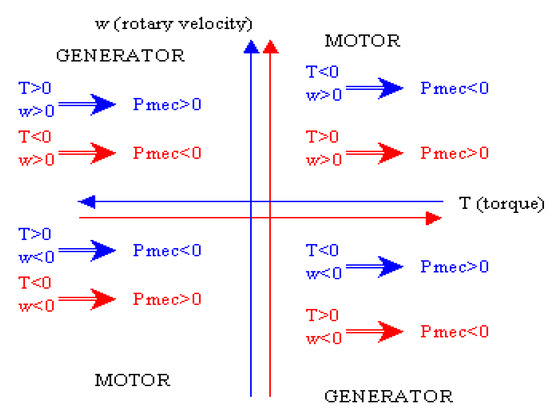
Figure 4. Electric motor operation.

Therefore, the relationship between mechanical power and electrical power, taking the below conditions into account, is as follows [62].

$$Pelec=Pmec-Plost$$

(44)

with

• $Pmec<0$ in engine mode.
• $Pmec>0$ in generator mode.
• $Plost>0$.

The efficiency of the motor/generator, either user-defined or derived from $Plost$, corresponds to the following.

Motor mode [63]:

$$\eta =2-\frac{Pelec}{Pmec}$$

(45)

Generator mode:

$$\eta =PelecPmec$$

(46)

• Limitation

It is the responsibility of the user to ensure that the power loss is less than the input power, i.e.,

• $Plost<Pelec$ in engine mode.
• $Plost<Pmec$ in generator mode.
• Electric current

The output current I5 [A] is calculated as follows [63]:

$$I_5=\frac{Pmec-Plost}{U}$$

(47)

where U is the input voltage [V] and given by [64]

$$U=V_5-V_6$$

(48)

4.1.6. Battery

The following describes a battery sub-model, which includes an internal resistance model in the case of a variable voltage. Experimental data are required to define the open-circuit voltage and internal resistance. Furthermore, thermal effects can be taken into account. The open-circuit voltage and internal resistance can be temperature-dependent.

This battery is a concatenation of cells in series and in parallel.

Output potential:

If the voltage is fixed, then the potential at the positive pole is calculated as follows [65]:

$$V3=fixedvoltage+V2$$

(49)

where

$$V3=fixedcellvoltage\cdot Scell+V2$$

(50)

If the voltage is variable, then the potential at the positive pole is calculated as follows [66]:

$$Vtarget=OCVbat-Rbat\cdot I3$$

(51)

$$Vtarget=Scell\cdot \left(OCVcell-Rcell\cdot Icell\right)$$

(52)

$$Icell=\frac{I_3}{Pcell}$$

(53)

The voltage is calculated using the target V [67]:

$$\frac{dV}{dt}=\frac{Vtarget-V}{tau}$$

(54)

where

$$\frac{dV}{dt}=I3-\frac{\frac{Vtarget-OCVbat}{Rbat}}{Cfbat}$$

(55)

where

$$\frac{dV}{dt}=I3-\frac{\frac{Vtarget-OCVbat}{Rbat}}{Cfcell.\frac{\mathrm{Pcell}}{\mathrm{Scell}}}$$

(56)

and, finally,

$$V3=V+V2$$

(57)

• State of charge (SOC)

The SOC [%] of the battery is a variable state whose derivative is calculated as follows [68]:

$$\frac{dSOC}{dt}=-\frac{dq}{dt}\cdot \frac{100}{Cnom}$$

where $Cnom$is the nominal capacity [As]. This derivative is limited so that the state of charge remains within a range of [0;100%].

The DOD [%] is used as an input to read the open-circuit voltage and internal resistance data files. It is derived as follows:

$$DOD=100-SOC$$

(58)

• Charge used by the load

The charge used by charge q [As] (or the charge removed from the battery) is calculated as follows:

$$\frac{dq}{dt}=-I3$$

(59)

where I3 is the battery current at port 3 [A].

Note that with the TM software conditions, the battery will discharge when the battery current at port 3, I3, is negative.

• Output power at port 1

The output power P [W] at port 1 is calculated as follows [67,68]:

$$P=Rbat\cdot I_3^2$$

(60)

where

$$P=Rcell\cdot Icel{l}^2\cdot Scell\cdot Pcell$$

(61)

5. Results and Discussion

The simulations were carried out for a low-cost tractor. The driving cycle adopted was 300 s. Additionally, the maximum working speed was specific for each tool attached to the tractor, as shown in Table 2. According to the optimal torque distribution, we found that the hybrid tractor had the following main features. The electric motor starts the tractor up to a certain power, or the combustion engine is switched on to provide traction and simultaneously recharge the battery via a generator. At a certain stabilized and low tractor power, the traction is in pure electric mode. All decelerations of the vehicle are provided by the electric motor, thus recovering the braking energy.

5.1. Tractor without Attached Tools

In this simulation, the tractor did not have any tools attached to it and had a variable speed, as shown in Figure 5 below. The maximum speed was 30 km/h.

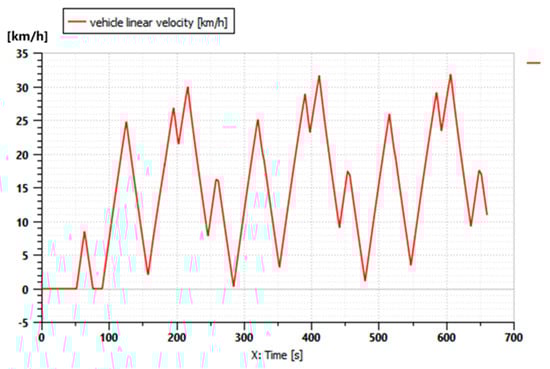
Figure 5. Tractor driving cycle without any attached implements.

Figure 6 shows the torque engine variation during the driving cycle described in Figure 5 when there are no implements attached to the tractor.

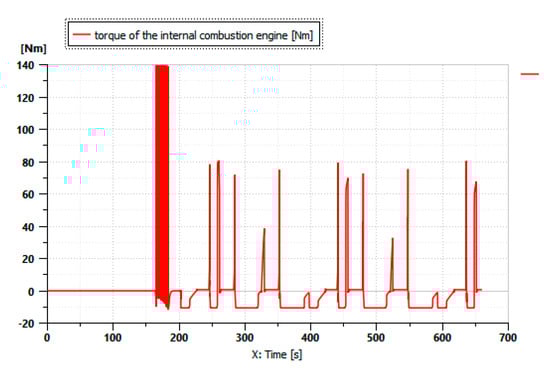
Figure 6. Thermal engine torque.

Figure 7 shows the variation in the torque of the electric motor during the driving cycle described in Figure 5 when there are no implements attached to the tractor.

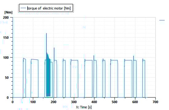
Figure 7. Electric motor torque.

The states of the vehicle’s engines confirm the results of the simulation. As illustrated in Figure 7, the electric motor continuously contributes throughout the driving cycle. Additionally, Figure 6 reveals a load for the internal combustion engine only after 180 s at high power demands. The generator is activated when the internal combustion engine is running to store energy in the battery. The role of the battery is to supply power to the electric motor. It should be noted that the addition of the electric motor significantly reduces the use of the internal combustion engine, and it is even possible to realize an all-electric operation.

Figure 8 shows the variation in the battery’s state of charge during the driving cycle shown in Figure 5 when there are no implements attached to the tractor.

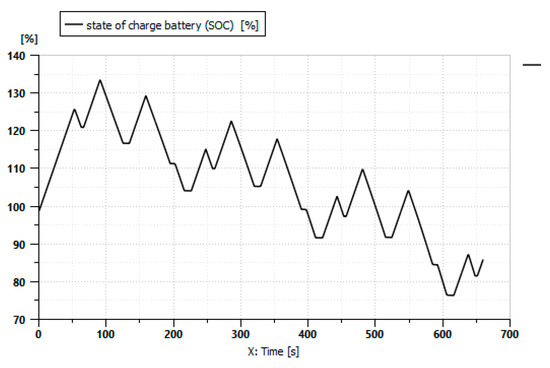
Figure 8. Battery’s state of charge.

Figure 8 shows the battery’s state of charge (%) during the mission profile. The SOC begins at 100%, and the operating range is between 100% and 75%.

Figure 9 shows the total fuel consumption during the driving cycle shown in Figure 5 when there are no implements attached to the tractor.

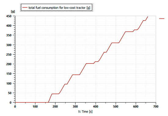
Figure 9. Fuel consumption.

Thus, fuel is not consumed until after 170 s of operation, as shown in Figure 9.

The downward trend in the curve reflects the nature of the discharge during the simulation period. The fluctuating SOC is caused by the battery being powered by the recuperative generator. Because the battery’s operating limit is at a low SOC level, the tractor reaches a point at which the engine must start. Therefore, the all-electric mode time in this driving cycle is 170 s (Thermal Engine Status).

Figure 10 illustrates the variation in the CO₂ released during the adopted mission profile. The curve shows an emission of 0 g for 170 s of operation; this is the result of the 100% electric operation, which minimizes the emissions rate.

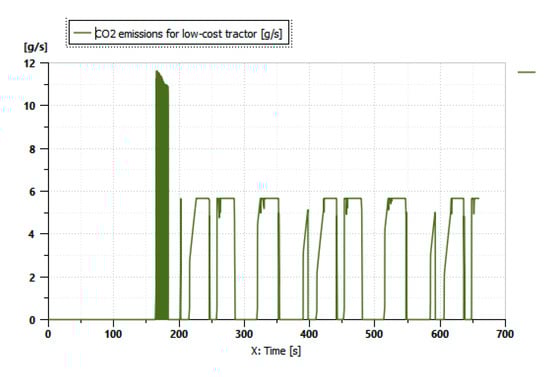
Figure 10. The variation in the CO₂ release.

5.2. Tractor with a Moldboard Plow

In this simulation, the moldboard plow tool was attached to the tractor. The speed was variable and had a maximum of 7 km/h, as shown in Figure 11 below.

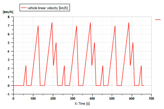
Figure 11. Tractor driving cycle with a moldboard plow attached.

Figure 12 shows the variation in the torque of the internal combustion engine during the driving cycle described in Figure 11 when a moldboard plow is attached to the tractor.

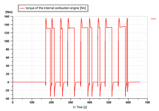
Figure 12. Thermal engine torque.

Figure 13 shows the variation in the torque of the electric motor during the driving cycle in Figure 11 when a moldboard plow is attached to the tractor.

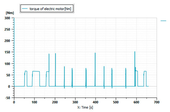
Figure 13. Electric motor torque.

The simulation results in Figure 13 show that the electric motor continuously contributes throughout the driving cycle, and it operates alone for 150 s. Figure 12 reveals a load for the internal combustion engine only at high power demands. With the generator functioning during operation, the internal combustion engine ensures that energy is stored in the battery, which is responsible for supplying power to the electric motor. The addition of the electric motor significantly reduces the use of the internal combustion engine.

Figure 14 shows the variation in the battery’s state of charge during the driving cycle in Figure 11 when a moldboard plow is attached to the tractor.

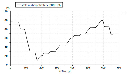
Figure 14. Battery’s state of charge.

Figure 14 shows the variation in total fuel consumption during the driving cycle in Figure 11 when a moldboard plow is attached to the tractor.

Figure 14 shows the battery’s state of charge (%) during the mission profile. The SOC starts at 100%. The operating range is between 100% and 10% and then increases because of the contribution of the combustion engine. Thus, fuel is consumed only after 170 s of operation, as shown in Figure 15. The downward trend in the curve reflects the nature of the discharge during the simulation period. The fluctuating SOC is caused by the battery being powered by the recuperative generator. Because the battery’s operating limit is at a low SOC level, the tractor reaches a point at which the engine must start. Therefore, the all-electric mode lasts for 150 s in this driving cycle (Thermal Engine Status).

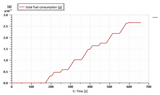
Figure 15. Fuel consumption.

Figure 16 illustrates the variation in the CO₂ released during the mission profile illustrated in Figure 11. The curve shows an emission of 0 g for 170 s of operation; this is the result of the 100% electric operation, which minimizes the emissions rate.

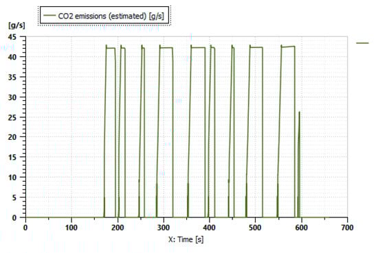
Figure 16. The variation in the CO₂ release.

5.3. Tractor with the Bette Harvest

In this simulation, the Bette Harvest variable-speed implement was attached to the tractor, as shown in Figure 17. The maximum speed was 9 km/h.

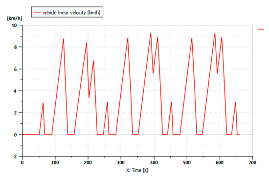
Figure 17. Tractor driving cycle with a Bette Harvest attached.

Figure 18 shows the variation in the torque of the internal combustion engine during the driving cycle described in Figure 17 when a Bette Harvest is attached to the tractor.

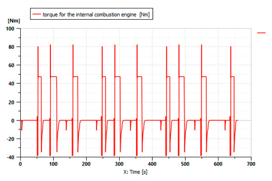
Figure 18. Thermal motor torque.

Figure 19 shows the variation in the torque of the electric motor during the driving cycle described in Figure 17 when a Bette Harvest is attached to the tractor.

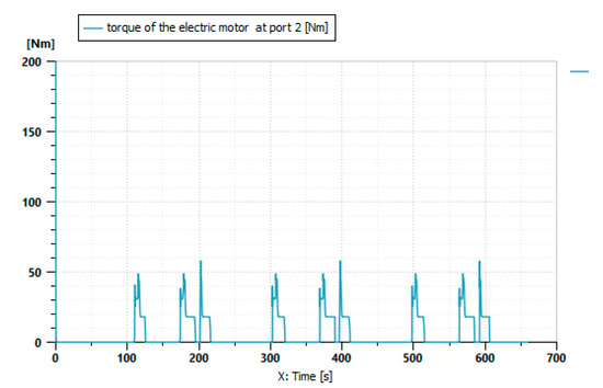
Figure 19. Electric motor torque.

The simulation results in Figure 19 show that the electric motor contributes little power during the driving cycle due to the high power demand of the tool. Figure 18 reveals that the internal combustion engine contributes in this cycle. With the generator functioning during the operation of the combustion engine, energy is stored in the battery, which supplies power to the electric motor. These results show that the addition of the electric motor significantly reduces the use of the combustion engine.

Figure 20 shows the variation in the battery’s state of charge during the driving cycle described in Figure 17 when a Bette Harvest is attached to the tractor.

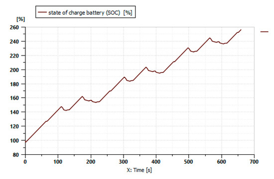
Figure 20. Battery’s state of charge.

Figure 21 shows the variation in total fuel consumption during the driving cycle described in Figure 17 when a Bette harvest is attached to the tractor.

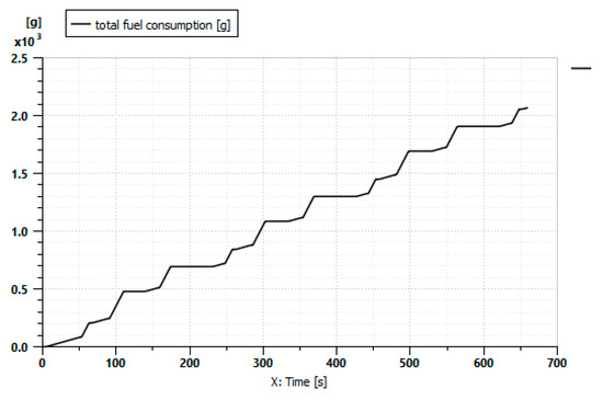
Figure 21. Fuel consumption.

Figure 20 shows the battery’s state of charge (%) during the mission profile. The SOC starts at 100%, and the operating range is higher than the highest engine contribution. The fuel consumption of the internal combustion engine is very high because of the high-power requirement, as shown in Figure 21.

Figure 22 illustrates the variation in CO₂ emissions during the adopted mission profile. The curve illustrates continuous and high CO₂ emissions, which is explained by the considerable intervention of the combustion engine.

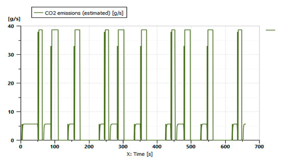
Figure 22. The variation in the CO₂ release.

5.4. Tractor with a Straw Tub grinder

In this simulation, the straw tub grinder tool was attached to the tractor. The tool does not require any movement, as shown in Figure 23.

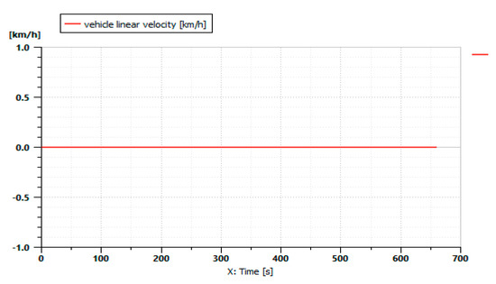
Figure 23. Tractor driving cycle with a straw tub grinder attached.

Figure 24 shows the variation in the torque of the internal combustion engine during the driving cycle described in Figure 23 when a straw tub grinder is attached to the tractor.

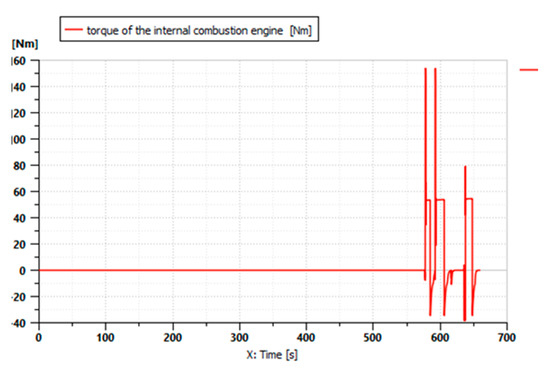
Figure 24. Thermal engine torque.

Figure 25 shows the variation in the torque of the electric motor during the driving cycle described in Figure 23 when a straw tub grinder is attached to the tractor.

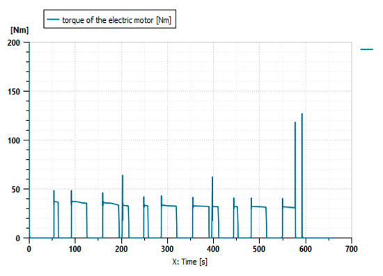
Figure 25. Electric motor torque.

The simulation results in Figure 25 show that the electric motor contributes substantially during the driving cycle because of the low power demand of the tool. However, the combustion engine contributes after 570 s, which is after the battery is discharged, as shown in Figure 24.

Figure 26 shows the battery’s state of charge (%) during the mission profile. The SOC starts at 100%. The operating range decreases because of the large contribution of the electric motor. Fuel is not consumed until 570 s, when the battery is discharged and the internal combustion engine starts to operate, as shown in Figure 27.

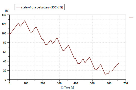
Figure 26. Battery’s state of charge.

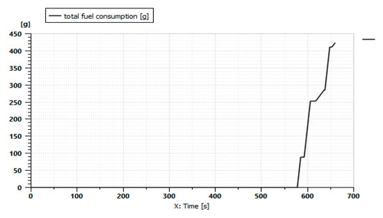
Figure 27. Fuel consumption.

Figure 28 illustrates the variation in CO₂ emissions during the adopted mission profile. The curve shows that CO₂ is not emitted until 570 s, which is when the combustion engine starts to operate and the battery is discharged.

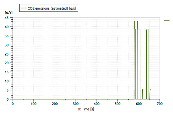
Figure 28. The variation in the CO₂ release.

6. Conclusions

Agriculture is one of the most important industries in the world, and the tractor is regarded as the main axial machine used in this sector.

The present work reports an evaluation of a low-cost tractor that is equipped with a parallel hybrid engine. Simulations were carried out with AMESim software with three different implements attached to the tractor. Each implement requires a different type of power.

First, without any attached implements, the tractor was able to run for 170 s with the electric motor only. This saved fuel during this period.

The second simulation was carried out with a moldboard plow attached to the tractor, which requires draft power. The simulation showed that the tractor worked with the electric motor for 150 s, which reflects notable fuel savings.

In the third simulation, the tractor was attached to a Bette Harvest, which requires draft power and PTO at the same time. Thus, very high power was required, and it could only be provided by placing a demand on both engines.

In the final simulation, the straw tub grinder was used, which only needs PTO. During the operation, the electric motor ran alone until the battery was discharged. Thereafter, the combustion engine started to operate and charged the battery.

Finally, the parallel hybrid architecture can minimize fuel consumption through the participation of the electric motor. H. Fathollahzadeh et al. found that when working the soil with a conventional tractor attached to a moldboard plow, the average fuel consumption was 30 L/ha, whereas the average fuel consumption by our low-cost tractor was 17 L/ha while performing the same work. This represents a significant decrease in consumption and emissions [69]. This improvement is the result of the power obtained by recovering energy from the combustion engine. The possibility of integrating renewable energy into our architecture will be the subject of our future work.

References

- Paillard, S. Agrimonde—Scenarios and Challenges for Feeding the World in 2050; Springer Science and Business Media: Berlin/Heidelberg, Germany, 2014. [Google Scholar]
- Alexandratos, N.; Bruinsma, J. World Agriculture towards 2030/2050; Food and Agriculture Organization of the United Nations: Roma, Italy, 2012. [Google Scholar]
- Food and Agriculture Organization of the United Nations. The Future of Food and Agriculture—Trends and Challenges; FAO: Rome, Italy, 2017. [Google Scholar]
- Kormawa, P. La Mécanisation Agricole Durable Cadre Stratéguique pour L’Afrique; FAO: Rome, Italy, 2019. [Google Scholar]
- Renius, K.T. Fundamentals of Tractors Design; Springer International Publishing: Cham, Switzerland, 2020. [Google Scholar]
- Tordo, S.; Lorenzato, G.; Zhao, J.; McEneaney, K.; Sarmiento-Saher, S.P. Options for Increased Private Sector in Resilience Investment Focus on Agriculture; World Bank: Washington, DC, USA, 2017. [Google Scholar]
- Salvat, B. Tracteurs Agricoles Renault; France Agricole: Paris, France, 2012. [Google Scholar]
- Sakai, J. Tractors: Two-wheel tractors for wet land farming. In Handbook of Agriculture Engineering; International Commission of Agricultural and Biosystems Engineering (CIGR): Liege, Belgium, 1999; Volume III, pp. 54–95. [Google Scholar]
- Karner, J.; Baldinger, M.; Schober, P.; Reichl, P.H. Hybrid systems for agricultural engineering. Landtechnik 2013, 68, 22–25. [Google Scholar]
- Karner, M.J. Prospects of hybrid systems on agricultural machinery. J. Agric. Eng. 2014, 1, 33–37. [Google Scholar] [CrossRef]
- Office of Mobile Sources. Non-Road Engines and Air Pollution; Environmental Protection Agency (EPA): Washington, DC, USA, 1669.
- Kannusamy, M.Y.L.; Ravindran, V.; Rao, N. Analysis of Multiple Hybrid Electric Concept in Agricultural Tractor through Simulation Technique; SAE International: Warrendale, PA, USA, 2019. [Google Scholar]
- Zahidi, Y.; Benhadou, S.; Medromi, H. Determining the optimal motorization for low-cost tractor. Int. J. Simul. Syst. Sci. Technol. 2020, 21, 1–13. [Google Scholar]
- Wang, L.; Zhang, Y.; Yin, C.; Zhang, H.; Wang, C. Hardware-in-the-loop simulation for the design and verification of the control system of a series–parallel hybrid electric city-bus. Simul. Model. Pract. Theory 2012, 25, 148–162. [Google Scholar] [CrossRef]
- Inoue, H. Development of hybrid hydraulic excavators. In Proceedings of the 9th JFPS International Symposium, Matsue, Japan, 28–31 October 2014. [Google Scholar]
- Zhang, B.; Guo, S.; Zhang, X.; Xue, Q.; Teng, L. Adaptive smoothing power following control strategy based on an optimal efficiency map for a hybrid electric tracked vehicle. Energies 2020, 13, 1893. [Google Scholar] [CrossRef]
- Ceresoli, F. Excavator with Two or Three Arms: Dynamical Behavior and Structural Implications; Department of Mechanical and Industrial Engineering, University of Brescia: Brescia, Italy, 2020. [Google Scholar]
- Wang, D.; Lu, X.; Wang, H.; Chen, M. A new design of foaming agent mixing device for a pneumatic foaming system used for mine dust suppression. Int. J. Min. Sci. Technol. 2016, 26, 187–192. [Google Scholar] [CrossRef]
- Shen, W.; Jiang, J.; Su, X.; Karimi, H.R. Control strategy analysis of the hydraulic hybrid excavator. J. Frankl. Inst. 2014, 352, 541–561. [Google Scholar] [CrossRef]
- Lin, T.; Wang, Q.; Hu, B.; Gong, W. Development of hybrid powered hydraulic construction machinery. Autom. Constr. 2020, 19, 11–19. [Google Scholar] [CrossRef]
- Choi, J.; Kim, H.; Yu, S.; Yi, K.C. Development of integrated controller for a compound hybrid excavator. J. Mech. Sci. Technol. 2011, 25, 1557. [Google Scholar] [CrossRef]
- Yoon, J.I.; Truong, D.Q.; Ahn, K.K. A generation step for an electric excavator with a control strategy and verifications of energy consumption. Int. J. Precis. Eng. Manuf. 2013, 14, 755–766. [Google Scholar] [CrossRef]
- Zeng, X.; Yang, N.; Peng, Y.; Zhang, Y.; Wang, J. Research on energy saving control strategy of parallel hybrid loader. Autom. Constr. 2014, 38, 100–108. [Google Scholar] [CrossRef]
- Hui, J.J.S. Research on the system configuration and energy control strategy for parallel hydraulic hybrid loader. Autom. Constr. 2010, 19, 100–108. [Google Scholar] [CrossRef]
- Dagci, O.H.; Peng, H.; Grizzle, J.W. Power-Split Hybrid Electric Powertrain Design with Two Planetary Gearsets for Light-Duty Truck Applications; International Federation of Automatic Control (IFAC): New York, NY, USA, 2015; pp. 8–15. [Google Scholar]
- van Keulen, T.; van Mullem, D.; de Jager, B.; Kessels, J.T.; Steinbuch, M. Design, implementation, and experimental validation of optimal power split control for hybrid electric trucks. Control Eng. Pract. 2012, 20, 547–558. [Google Scholar] [CrossRef]
- Bodria, L. Evolution and Prospects of Agricultural Mechanization in the World; Italian Agriculture Machinery Manufacture Federation: Boulogne, Italy, 2016. [Google Scholar]
- Ehsani, M.; Gao, Y.; Miller, J.M. Hybrid electric vehicles: Architecture and motor drives. Proc. IEEE 2007, 95, 719–728. [Google Scholar] [CrossRef]
- Modern, C.K. Electric Vehicle Technology; Springer: New York, NY, USA, 2001. [Google Scholar]
- American Society of Agricultural and Biological Engineers. Agricultural Machinery Management Data; American Society of Agricultural Engineers: St. Joseph, MI, USA, 2000. [Google Scholar]
- Baek, S.W.; Lee, S.W. Aerodynamic drag reduction on a realistic vehicle using continuous. Microsyst. Technol. 2019, 26, 11–23. [Google Scholar] [CrossRef]
- Khanipour, A.; Ebrahimi, K.M.; Seale, W.J. Conventional design and simulation of an urban hybrid bus. Int. J. Mech. Mechatron. Eng. 2007, 1, 147. [Google Scholar]
- Szadkowski, B.; Chrzan, P.J.; Roye, D. A study of energy requirements for electric and hybrid vehicles in cities. In Proceedings of the 2003 International Conference on Clean, Efficient and Safe Urban Transport, Gdansk, Poland, 4–6 June 2003. [Google Scholar]
- Bissam, A. Étude et Commande des Véhicules Hybrides Parallèles; Université de Bejaïa: Bejaïa, Algery, 2013. [Google Scholar]
- Ehsani, M.; Gao, Y.; Longo, S.; Ebrahimi, K. Modern Electric, Hybride Electric and Fuel Cell Vehicles; CRC Press: Boca Raton, FL, USA, 2005. [Google Scholar]
- Bouzidi, I. Etude des Vibrations Libres D’une Boite de Vitesse Par la Méthode des Éléments Finis. Ph.D. Thesis, The Universite Abou Bekr Belkaid-Tlemcenfaculte De Technologie, Chetouane, Algery, 2013. [Google Scholar]
- Dion, J.L.; Le Moyne, S.; Chevallier, G.; Sebbah, H. Gear impacts and idle gear noise: Experimental study and non linear dynamic model. Mech. Syst. Signal Process. 2009, 23, 2608–2628. [Google Scholar] [CrossRef]
- Mèmeteau, H.B. Technologie Fonctionnelle de L’automobile: Transmission, Train Roulant et Equipement Electrique; Dunod: Paris, France, 2014. [Google Scholar]
- Martin, M.R.; Hoeijmakers, J. The electrical variable transmission in a city bus. In Proceedings of the 35th Annual IEEE Power Electronics Specialists Conference, Aachen, Germany, 20–25 June 2004. [Google Scholar]
- Kowalak, P.; Borkowski, T.; Bonisławski, M.; Hołub, M.; Myśków, J. A statistical approach to zero adjustment in torque measurement of shippropulsion shafts. Measurement 2020, 164, 108088. [Google Scholar] [CrossRef]
- Tamada, S.; Bhattacharjee, D.; Dan, P.K. Review on automatic transmission control in electric and non-electric automotive powertrain. Int. J. Veh. Perform. 2020, 6, 98–128. [Google Scholar] [CrossRef]
- Adeline, A. Modelisation Dynamique Globale des Boites de Vitesses Automobile; L’Institut National des Sciences Appliquees de Lyon: Lyon, France, 1997. [Google Scholar]
- Barathiraja, K.; Devaradjane, G.; Paul, J.; Rakesh, S.; Jamadade, G. Analysis of automotive transmission gearbox synchronizer wear due to torsional vibration and the parameters influencing wear reduction. Eng. Fail. Anal. 2019, 105, 427–443. [Google Scholar]
- Hridoy, S.A.A. Lightweight Authenticated Encryption for Vehicle Controller Area Network. Ph.D. Thesis, The Queen’s University, Kingston, ON, Canada, 2020. [Google Scholar]
- Kaveh, M.; Abbaspour-Gilandeh, Y. Impacts of hybrid (convective-infrared-rotary drum) drying on the quality attributes of green pea. J. Food Process. Eng. 2020, 43, e13424. [Google Scholar] [CrossRef]
- Baytorun, A.N.; Zaimoğlu, Z.; Akyüz, A.; Üstün, S.; Çaylı, A. Comparison of greenhouse fuel consumption calculated using different methods with actual fuel consumption. Turk. J. Agric. Food Sci. Technol. 2018, 7, 850–857. [Google Scholar] [CrossRef][Green Version]
- Hansson, P.A.; Lindgren, M.; Norén, O. A comparison between different methods of calculating average engine emissions for agricultural tractors. J. Agric. Eng. 2001, 1, 80. [Google Scholar]
- Coelho, M.C.; Farias, T.L.; Rouphail, N.M. Effect of roundabout operations on pollutant emissions. Transp. Res. D Transp. Environ. 2006, 11, 333–343. [Google Scholar] [CrossRef]
- Galindo, J.; Lujan, J.M.; Serrano, J.R.; Dolz, V.; Guilain, S. Description of a heat transfer model suitable to calculate transient processes of turbocharged diesel engines with one-dimensional gas-dynamic codes. Appl. Therm. Eng. 2006, 26, 66–76. [Google Scholar] [CrossRef]
- Açıkgöz, B.; Çelik, C.; Soyhan, H.S.; Gökalp, B.; Karabağ, B. Emission characteristics of a hydrogen–CH4 fuelled spark ignition engine. Fuel 2015, 159, 298–307. [Google Scholar] [CrossRef]
- Chewning, S.R. Micro Adiabatic Combustion Engine: Concept Development, Simulation and Combustion Experiments. Ph.D. Thesis, Oregon State University, Corvallis, OR, USA, 2009. [Google Scholar]
- Abedin, M.J.; Masjuki, H.H.; Kalam, M.A.; Sanjid, A.; Rahman, S.A.; Masum, B.M. Energy balance of internal combustion engines using alternative fuels. Int. J. Simul. Syst. Sci. Technol. 2013, 26, 20–33. [Google Scholar] [CrossRef]
- Bertana, M.; Truchot, B.; Marlair, G. Comparison of the fire consequences of an electric vehicle and an internal combustion engine vehicle. In Proceedings of the International Conference on Fires in Vehicles, Chicago, IL, USA, 27–28 September 2012. [Google Scholar]
- Janhunen, T.T. Ultra-Low Nox Hcci-Combustion in the Z Engine; SAE Technical Paper; SAE: Warrendale, PA, USA, 2012. [Google Scholar]
- Sim, K.; Koo, B.; Kim, C.H.; Kim, T.H. Development and performance measurement of micro-power packusing micro-gas turbine driven automotive alternators. Appl. Energy 2013, 103, 309–319. [Google Scholar] [CrossRef]
- Galindo, J.; Serrano, J.R.; Climent, H.; Varnier, O. Impact of two-stage turbocharging architectures on pumping losses of automotive engines based on an analytical model. Energy Convers. Manag. 2010, 51, 1958–1969. [Google Scholar] [CrossRef]
- Fu, J.; Liu, J.; Yang, Y.; Ren, C.; Zhu, G. A new approach for exhaust energy recovery of internal combustion engine: Steam turbocharging. Appl. Therm. Eng. 2013, 52, 150–159. [Google Scholar] [CrossRef]
- Boretti, A.; Scalco, J. Piston and Valve Deactivation for Improved Part Load Performances of Internal Combustion Engines; SAE International: Warrendale, PA, USA, 2011. [Google Scholar]
- Ibrahim, H.; Ilinca, A.; Perron, J. Moteur Diesel Suralimenté Bases et Calculs Cycles Réel, Théorique et Thermodynamique; Université du Québec à Rimouski: Rimouski, QC, Canada, 2006. [Google Scholar]
- Hanselman, D. Minimum torque ripple, maximum efficiency excitation of brushless permanent magnet motors. IEEE Trans. Ind. Electron. 1994, 41, 292–300. [Google Scholar] [CrossRef]
- Rigacci, M.; Sato, R.; Shirase, K. Experimental evaluation of mechanical and electrical power consumption of feed drive systems driven by a ball-screw. Precis. Eng. 2020, 64, 280–287. [Google Scholar] [CrossRef]
- Mohammed, K.G. Mechanical and electrical design calculations of hybrid vehicles. In Applied Electromechanical Devices and Machines for Electric Mobility Solutions; IntechOpen: London, UK, 2020. [Google Scholar]
- Chung, C.T.; Wu, C.H.; Hung, Y.H. Evaluation of driving performance and energy efficiency for a novel full hybrid system with dual-motor electric drive and integrated input- and output-split e-CVT. Energy 2020, 191, 116508. [Google Scholar] [CrossRef]
- Daguse, B. Modélisation Analytique Pour le Dimensionnement par Optimisation D’une Machine Dédiée à une Chaîne de Traction Hybride à Dominante Électrique. Ph.D. Thesis, Ecole Doctorale Sciences et Technologies de l’Information des Télécommunications et des Systèmes, Paris, France, 2013. [Google Scholar]
- Chouchane, M.; Primo, E.N.; Franco, A.A. Mesoscale effects in the extraction of the solid-state lithium diffusion coefficient values of battery active materials: Physical insights from 3D modeling. J. Phys. Chem. Lett. 2020, 11, 2775–2780. [Google Scholar] [CrossRef] [PubMed]
- Liu, Y.; Tang, S.; Li, L.; Liu, F.; Jiang, L.; Jia, M. Simulation and parameter identification based on electrochemical- thermal coupling model of power lithium ion-battery. J. Alloy. Compd. 2020, 844, 156003. [Google Scholar] [CrossRef]
- Li, A. Analyse Expérimentale et Modélisation d’Eléments de Batterie et de Leurs Assemblages: Application Aux Véhicules Electriques Et Hybrides. Ph.D. Thesis, L’Universite Claude Bernard, Lyon, France, 2006. [Google Scholar]
- Urbain, M. Modélisation Electrique et Energétique des Accumulateurs Li-Ion. Estimation en Ligne de la SOC et de la SOHL. Ph.D. Thesis, Institut National Polytechnique de Lorraine, Lorraine, France, 2009. [Google Scholar]
- Fathollahzadeh, H.; Mobli, H.; Rajabipour, A.; Minaee, S.; Jafari, A.; Tabatabaie, S.M.H. Average and instantaneous fuel consumption of Iranian conventional tractor with moldboard plow in tillage. ARPN J. Eng. Appl. Sci. 2010, 5, 30–35. [Google Scholar]
Publisher’s Note: MDPI stays neutral with regard to jurisdictional claims in published maps and institutional affiliations. |
© 2020 by the authors. Licensee MDPI, Basel, Switzerland. This article is an open access article distributed under the terms and conditions of the Creative Commons Attribution (CC BY) license (http://creativecommons.org/licenses/by/4.0/).