Automated Longitudinal Control Based on Nonlinear Recursive B-Spline Approximation for Battery Electric Vehicles

Abstract

This works presents a driver assistance system for energy-efficient automated longitudinal control (ALC) of a battery electric vehicle (BEV). The ALC calculates a temporal velocity trajectory from map data. The trajectory is represented by a cubic B-spline function and results from an optimization problem with respect to travel time, driving comfort and energy consumption. For the energetic optimization we propose an adaptive model of the required electrical traction power. The simple power train of a BEV allows the formulation of constraints as soft constraints. This leads to an unconstrained optimization problem that can be solved with iterative filter-based data approximation algorithms. The result is a direct trajectory optimization method of which the effort grows linearly with the trajectory length, as opposed to exponentially as with most other direct methods. We evaluate ALC in real test drives with a BEV. We also investigate the energy-saving potential in driving simulations with ALC compared to manual longitudinal control (MLC). On the chosen reference route the ALC saves up to $3.4\%$ energy compared to MLC at same average velocity, and achieves a $2.6\%$ higher average velocity than MLC at the same energy consumption.

1. Introduction

1.1. Driver Assistance Systems for Automated Longitudinal Control

Current major automotive trends are automated driving, electric power train, shared mobility services, and connected mobility [1]. Driver assistance systems are important intermediate steps of automated driving. The continuously increasing degree of automation provided by them leads the way to autonomous vehicles ([2], p. 89).

We can distinguish three classes of driver assistance systems regarding the vehicle guidance: First, informing and warning systems like traffic sign recognition. These only influence the vehicle via the driver. Second, continuously automated functions, that are activated by the driver intentionally and influence the vehicle directly. These are usually comfort functions like cruise control (CC). Third, intervening emergency functions like automatic emergency braking. These act in critical situations, over short time periods and are not deliberately activated by the driver ([2], pp. 36–40).

This work deals with continuously automated functions for longitudinal control. Such functions can contribute to increasing safety and comfort as well as to reducing energy consumption to different extents. Adaptive cruise control (ACC) is an enhanced CC that adapts the vehicle velocity to a preceding vehicle, which is detected by a radar sensor ([2], p. 1095). Studies report that drivers with activated ACC experience less mental stress and the number of forward collisions decreases by 35% ([2], p. 1140). With map data, ACC-like systems for automated longitudinal control (ALC) can determine an appropriate course of velocity, also refered to as velocity trajectory, for the upcoming road section such that the vehicle automatically slows down if a curve is ahead. In combination with power train models, such systems can guide the vehicle more energy-efficiently than a human driver. For example, the system described in [3,4] achieves, on average, a 10% lower energy consumption compared with a human driver at the same average velocity.

The degrees of freedom of the power train in a conventional vehicle include motor torque, clutch state and selected gear. In addition to that, a hybrid power train can transfer power between the combustion engine, electric motor and wheels in several ways. Due to the various degrees of freedom in the power train and the related constraints, the majority of such driver assistance systems determine the velocity trajectory by solving a multiobjective nonlinear high dimensional optimization problem with respect to goals like travel time, comfort, safety and energy consumption [5].

The three common approaches to trajectory optimization are dynamic programming (DP), direct methods (DM) and indirect methods (IM) ([6], pp. 5–8,27–37). DP is an optimization method that finds a global optimum. With DP, the complexity increases linearly with the length of the planned trajectory but exponentially with the problem dimensionality. ALC systems based on DP include the system in [3,4] for a vehicle with an internal combustion engine, the extension for a hybrid electric vehicle (HEV) in [7], and the system for a plug-in HEV in [8].

A comparison between an ALC based on DP with a spatially defined problem and an ALC based on model predictive control (MPC) with a temporally defined problem regarding the energy consumption of a battery electric vehicle (BEV) and the computation time is conducted in [9]. In simulations the vehicle requires 1.14% and 1.27% less energy with MPC ALC than with a proportional-integral-derivative controller that represents human driving behavior.

MPC is a representative of DM. With DM, the trajectory is defined by a function, of which the parameters are the optimization variables. DM find local optima, they have a polynomial increase of computational effort with the dimensionality, and their computational effort usually increases exponentially with the trajectory length. Further MPC-based ALC systems are proposed in [10] for HEVs and for BEVs in [11].

The ALC for fuel cell HEVs of [12] uses Pontryagin’s minimum principle, which belongs to IM. The effort of the locally optimal IM grows polynomially with the dimensionality and the trajectory length.

Apart from the aforementioned approaches, which can be seen as model-based methods, there are rule-based methods like the system proposed for an HEV in [13] and learning-based methods. For example, the behavior learning system reported in [14] uses a reinforcement learning technique to capture and replicate the difficult to model behavior of humans during longitudinal control and how they adapt their control to different driving situations. A driving style recognition algorithm based on unsupervised learning and its use within a codesign optimization for a BEV ALC is described in [15].

For a comprehensive review of motion planning techniques including the lateral dimension we refer to [16].

1.2. Research Gap

Most systems for energy-efficient ALC described in literature were developed for conventional vehicles or HEVs, which are vehicles with rather complicated power train structures. As a result, these systems usually solve high-dimensional optimization problems that involve models of several power train components, nonlinearities and constraints. In order to perform the required computations on an electronic control unit (ECU) with limited computational power in real-time, the trajectory optimization problem often needs to be simplified and discretized coarsely.

In contrast to conventional and hybrid vehicles, the power train of most BEVs has only a constant gear ratio and no clutch. The simple power train structure allows for less computational effort during trajectory optimization. However, the ALCs that have been proposed for BEVs are mostly based on MPC and therefore the optimization is restricted to short time horizons because of the exponential increase of computational effort.

An exception is the ALC for BEVs proposed in [17,18] that defines the trajectory as a cubic polynomial, of which the coefficients are determined by a linear Kalman filter. The iterative filter-based trajectory optimization approach results in a direct method with only a linear increase of complexity with the trajectory length. However, in practice this method is also restricted to short trajectories because the few degrees of freedom of the cubic polynomial do not allow representation of a farsighted trajectory that includes several acceleration and deceleration phases. In particular, the effectivenes of energy consumption optimization benefits greatly from a larger optimization horizon. The energy consumption is also not considered in [17,18].

The lack of systems for ALC of BEVs that take advantage of the simpler power train by using algorithms with low computational effort for planning long trajectories and that additionally consider the energy consumption in the optimization problem poses a research gap.

1.3. Contribution

In [19] we presented a method denoted recursive B-spline approximation (RBA) that iteratively adapts the coefficients of a B-spline function such that the function approximates data in the weighted least squares (WLS) sense. In [5] we proposed an analogous algorithm called nonlinear recursive B-spline approximation (NRBA) for nonlinear weighted least squares (NWLS) approximation problems. In both publications, we investigated the algorithms in numerical experiments and provided an implementation in Matlab. Furthermore, we applied NRBA to unconstrained nonlinear multiobjective trajectory optimization and demonstrated that NRBA can serve as an iterative local direct optimization method for B-spline trajectories. With NRBA, the computational effort only grows linearly with the time horizon instead of exponentially.

This publication describes a system for energy-efficient ALC of BEVs that is tested in simulation as well as in real test drives and aims to contribute to closing the identified research gap. The ALC computes a velocity trajectory with respect to time using map data and includes RBA and NRBA for trajectory optimization. The trajectory can be optimized with respect to travel time, driving comfort and energy consumption. We also propose an adaptive model that captures the characteristics of the BEV power train in an aggregated form and is used for determining energy-efficient trajectories.

The trajectory optimization method falls into the category of direct methods(DM) but its effort increases only in a linear fashion with the trajectory length. This substantial saving is achieved by taking advantage of the comparatively simple BEV power train and by defining constraints from vehicle dynamics or the environment as soft constraints. This allows the formulation of the trajectory optimization problem as an approximation problem and allows the application of the iterative filter-based algorithms, RBA and NRBA. These features in combination with the use of a B-spline function enable planning long, farsighted trajectories. An implementation of the method is again provided in Matlab.

On a chosen reference route, the BEV has a lower energy consumption with the proposed ALC than with manual longitudinal control (MLC) at the same average velocity.

1.4. Outline

The remainder of this article is structured as follows: In Section 2, we describe the BEV with which we tested the ALC, influence factors on the energy consumption of a BEV, and the approach for optimizing the energy consumption. Section 3 describes the architecture of the proposed ALC and its individual modules. In Section 4, we report on test drives, as well as acceptance test results, and investigate the energy-saving potential of the ALC on a reference route. We summarize and draw our conclusions in Section 5.

2. Energy Consumption of Battery Electric Research Vehicles

2.1. Research Vehicle

The research vehicle is an all-wheel-driven battery electric convertible based on the Porsche Boxster type 981, which was developed during the research project e-generation. The vehicle has one electric motor per axle, a constant gear ratio and no clutch [20,21,22].

2.2. Driving Resistances

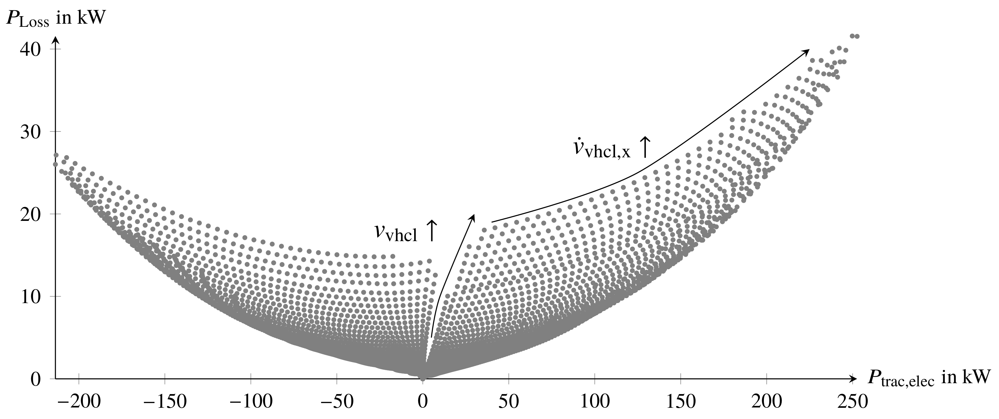
This section states the main forces acting on a vehicle during its operation. The climbing force $F_{\mathrm{cl}}$ with

$$F_{\mathrm{cl}}=m_{\mathrm{vhcl}}·g·sin\left(\alpha \right)$$

(1)

results from the gravitational force $m_{\mathrm{vhcl}}·g$, where $m_{\mathrm{vhcl}}$ is the vehicle mass, g is the gravitational constant, and $\alpha$ is the road slope angle. $\alpha$ is measured between the road surface and the plane that is perpendicular to the direction of gravitational force. The rolling resistance $F_{\mathrm{roll}}$ with

$$F_{\mathrm{roll}}=f_{\mathrm{r}}·m_{\mathrm{vhcl}}·g·cos\left(\alpha \right)$$

(2)

results from damping forces of the deformed tire rubber. $f_{\mathrm{r}}$ is the rolling resistance coefficient ([23], pp. 50–53). Without environmental wind, the air resistance $F_{\mathrm{air}}$ is given by

$$F_{\mathrm{air}}=\frac{\rho }{2}·c_{\mathrm{w}}·A·v_{\mathrm{vhcl}}^2.$$

(3)

$\rho$ is the air density, $c_{\mathrm{w}}$ is the aerodynamic drag coefficient that describes the shape of the vehicle, A denotes the effective vehicle cross-sectional area, and $v_{\mathrm{vhcl}}$ denotes the vehicle velocity ([24], pp. 212–214). The inertial force $F_{\mathrm{inert}}$ with

$$F_{\mathrm{inert}}=m_{\mathrm{vhcl}}·{\dot{v}}_{\mathrm{vhcl},\mathrm{x}}$$

(4)

occurs during vehicle longitudinal acceleration ${\dot{v}}_{\mathrm{vhcl},\mathrm{x}}$. Equation (4) neglects the equivalent inertial mass of rotating power train components ([25], pp. 16,17). The sum of these driving resistances equals the traction force $F_{\mathrm{trac}}$ between the tires and road surface:

$$F_{\mathrm{trac}}=F_{\mathrm{cl}}+F_{\mathrm{roll}}+F_{\mathrm{air}}+F_{\mathrm{inert}}.$$

(5)

The corresponding mechanical traction power $P_{\mathrm{trac},\mathrm{mech}}$ provided by the power train ([23], pp. 50–53) reads

$$P_{\mathrm{trac},\mathrm{mech}}=F_{\mathrm{trac}}·v_{\mathrm{vhcl}}.$$

(6)

2.3. Power Train

The power train of a BEV converts electrical traction power $P_{\mathrm{trac},\mathrm{elec}}$ from the high voltage (HV) battery into mechanical traction power $P_{\mathrm{trac},\mathrm{mech}}$ for vehicle propulsion. For recuperative braking, the power conversion is reversed. Losses from mechanical power train components include friction losses in the gearbox, which increase with rotation speed and transmitted torque, whereas the internal ohmic resistance contributes to the losses from the electrical power train components ([26], pp. 9–19). We denote the power loss between the HV battery and wheels with $P_{\mathrm{Loss}}$:

$$P_{\mathrm{Loss}}=P_{\mathrm{trac},\mathrm{elec}}-P_{\mathrm{trac},\mathrm{mech}}.$$

(7)

2.4. Energy Consumption and Optimization Approach

The HV battery energy $E_{\mathrm{Batt}}$ required for a route, is determined by integrating the HV battery power $P_{\mathrm{Batt}}$ over time t, whereby $t_{\mathrm{Trip}}$ denotes the trip time:

$$E_{\mathrm{Batt}}={\int }_{t=0}^{t_{\mathrm{Trip}}}{P}_{\mathrm{Batt}}\left(t\right)\mathrm{d}t.$$

(8)

This work focuses on optimization of the energy consumption for vehicle propulsion and assumes that $P_{\mathrm{Batt}}=P_{\mathrm{trac},\mathrm{elec}}$. The power required for auxiliaries, such as heating of the passenger cabin, and HV battery, as well as the air conditioning compressor can contribute a significant amount to the total energy consumption for a trip [27], but this is not considered as it varies strongly with environmental conditions and personal comfort requirements.

Figure 1 depicts $P_{\mathrm{Loss}}$ with respect to $P_{\mathrm{trac},\mathrm{elec}}$. The data points result from computing driving resistances and power train quantities, with a detailed power train model for various combinations of $v_{\mathrm{vhcl}}$ and ${\dot{v}}_{\mathrm{vhcl},\mathrm{x}}$ with $\alpha =0$. Arrows indicate the effects of increasing $v_{\mathrm{vhcl}}$ and ${\dot{v}}_{\mathrm{vhcl},\mathrm{x}}$. $P_{\mathrm{Loss}}$ increases progressively with increasing absolute value of $P_{\mathrm{trac},\mathrm{elec}}$, and therefore the efficiency $P_{\mathrm{trac},\mathrm{mech}}/P_{\mathrm{trac},\mathrm{elec}}$ of the power conversion decreases.

In the ALC we use $P_{\mathrm{trac},\mathrm{elec}}$ as a measure for $P_{\mathrm{Loss}}$, create a mathematical model of $P_{\mathrm{trac},\mathrm{elec}}$ and penalize the absolute value of $P_{\mathrm{trac},\mathrm{elec}}$ during trajectory optimization, to such an extent that the ALC avoids inefficient power peaks with a negligible effect on the trip time.

The reason for using $P_{\mathrm{trac},\mathrm{elec}}$ as a criterion is that $P_{\mathrm{trac},\mathrm{elec}}$ can be determined during vehicle operation from sensor measurements, which does not apply to $F_{\mathrm{trac}}$ and $P_{\mathrm{trac},\mathrm{mech}}$. The criterion must be measurable in order to be able to use a model that adapts its parameters during vehicle operation. This adaption is neccessary for an accurate model because the vehicle parameters $m_{\mathrm{vhcl}}$, $f_{\mathrm{r}}$ and $\frac{\rho }{2}·c_{\mathrm{w}}·A$ can change and $P_{\mathrm{trac},\mathrm{elec}}$ also depends on these parameters.

Even without explicit consideration of the power demand of auxiliaries in the ALC, the penalization of $P_{\mathrm{trac},\mathrm{elec}}$ is beneficial for efficiency because any additional consumption of auxiliaries further increases $P_{\mathrm{Loss}}$.

3. Automated Longitudinal Control System

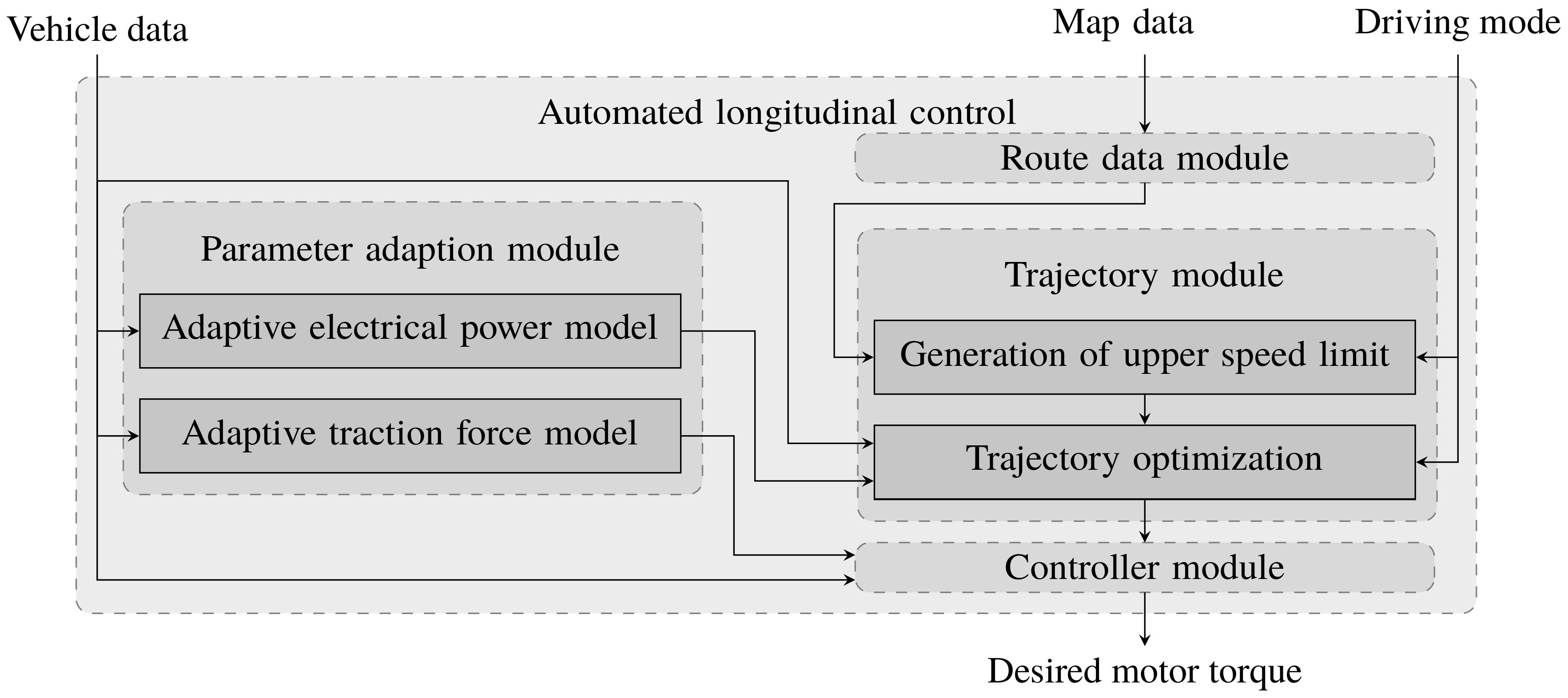
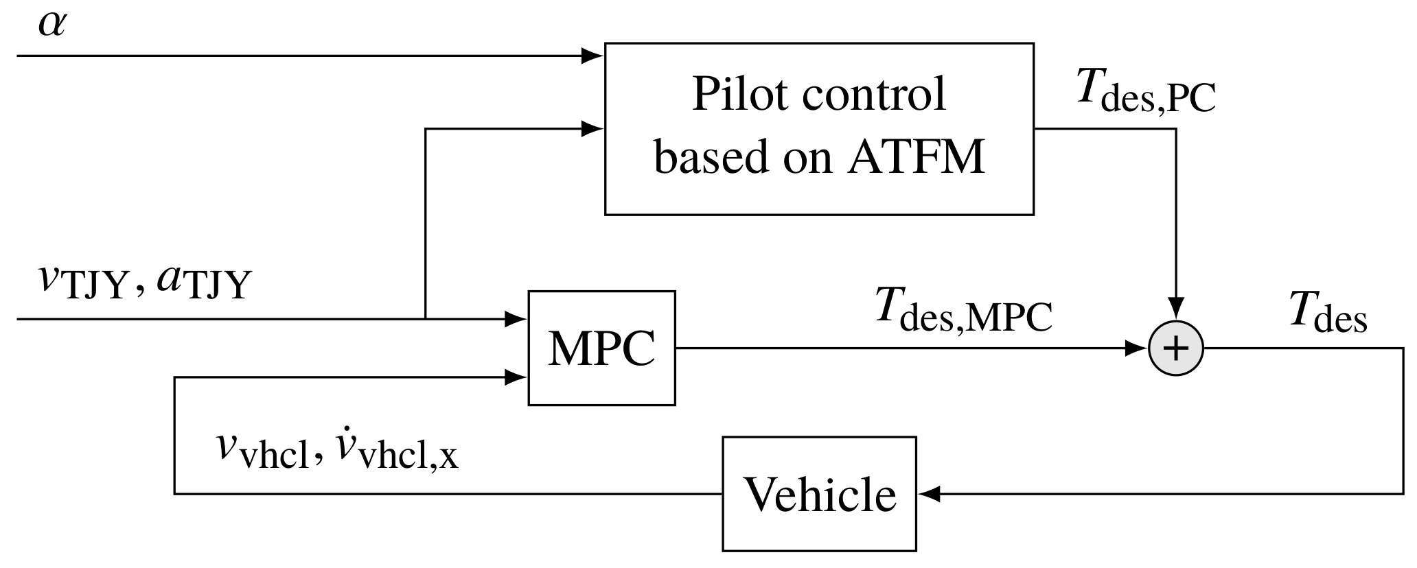
3.1. System Architecture

Figure 2 depicts the system architecture of the ALC that computes the desired motor torque depending on vehicle data, map data and the chosen driving mode. The ALC consists of the route data module, parameter adaption module, trajectory module and controller module. The following sections describe each module in detail.

The ALC is integrated into a Matlab-Simulink framework that runs on the rapid prototyping ECU ETAS ES910. The framework performs the correct communication via the controller area network (CAN) bus and abstracts CAN messages to signals with physical units. Additionally, the framework includes a plausibilisation and safety limitation of the motor torque demand of the ALC in order to enable both a safe vehicle operation and dynamic development of the ALC.

3.2. Parameter Adaption Module

The parameter adaption module updates two adaptive vehicle models every 50 ms using vehicle data from the CAN bus. For a given driving situation, the adaptive traction force model (ATFM) computes the required traction force $F_{\mathrm{trac}}$, and the adaptive electrical power model (AEPM) computes the required electrical traction power $P_{\mathrm{trac},\mathrm{elec}}$.

Both quantities depend on the driving resistances that are also affected by the vehicle parameters $m_{\mathrm{vhcl}}$, $f_{\mathrm{r}}$ and $\frac{\rho }{2}·c_{\mathrm{w}}·A$. These parameters are not exactly known during vehicle operation because they change with the number of passengers, amount of luggage, tire temperature and state of the convertible top. Therefore we develop adaptive models that estimate these parameters either explicitely or in aggregated form.

In order to be able to adapt a model, its inputs and outputs must be quantities that can be derived from signals on the CAN bus. For an update of the ATFM we use the vehicle velocity $v_{\mathrm{vhcl}}$, the longitudinal specific acceleration $a_{\mathrm{x}}$, the front axle motor torque $T_{\mathrm{EM},\mathrm{FA}}$ and the rear axle motor torque $T_{\mathrm{EM},\mathrm{RA}}$. An update of the AEPM requires $v_{\mathrm{vhcl}}$, $a_{\mathrm{x}}$ and the voltages and currents of the electric motors.

$v_{\mathrm{vhcl}}$ is computed from wheel speed sensor measurements and $a_{\mathrm{x}}$ is measured by the acceleration sensor. Due to its measurement principle, the sensor value is influenced by both inertial and gravitional force. Therefore $a_{\mathrm{x}}$ roughly equals

$$a_{\mathrm{x}}={\dot{v}}_{\mathrm{vhcl},\mathrm{x}}+g·sin\left(\alpha \right).$$

(9)

$T_{\mathrm{EM},\mathrm{FA}}$ and $T_{\mathrm{EM},\mathrm{RA}}$ are not measured but are computed by the motor ECU using measured motor voltages and currents in combination with look-up tables.

Before CAN signals are used for updating the models, we remove signal noise using the polynomial Kalman smoother of [28]. In two situations the models are not adapted: First, during a vehicle standstill because the missing excitation in the data can cause the models to diverge. Second, if CAN signals indicate that there is significant hydraulic brake pressure. This is because the models only consider braking via recuperation and are not valid while hydraulic brakes activated. The models do not take into account the hydraulic brakes as we need knowledge about the friction coefficient between brake disc and brake pad in order to calculate the hydraulic brake torque from brake pressure. This friction coefficient, however, is not constant and therefore has to be estimated as well [29]. Therefore, we only update the models without presence of the additional uncertainty of the friction coefficient.

Outputs of the parameter adaption module are updated parameters of ATFM and AEPM. Section 3.3 describes the ATFM and Section 3.4 the AEPM.

A comprehensive review of vehicle energy consumption models including a classification and an analysis of influence factors on the energy consumption is given in [30]. Based on the criteria in [30], the ATFM is a gray-box model and the AEPM a vehicle-based black-box consumption model.

3.3. Adaptive Traction Force Model

The ATFM answers the question of how much traction force is needed for a given combination of $v_{\mathrm{vhcl}}$ and $a_{\mathrm{x}}$. The ATFM is used by a pilot control in the controller module of the ALC. The ATFM is based on a simplification of (5). For small slope angles $cos\left(\alpha \right)\approx 1$ applies, hence we can approximate the rolling resistance by the rolling resistance contant $F_0$. Furthermore, the inertial force and climbing force can be merged using (9). The traction force $F_{\mathrm{trac}}$ can be computed as

$$F_{\mathrm{trac}}=T_{\mathrm{EM},\mathrm{FA}}·\frac{i_{\mathrm{G}}}{r_{\mathrm{dyn},\mathrm{FA}}}+T_{\mathrm{EM},\mathrm{RA}}·\frac{i_{\mathrm{G}}}{r_{\mathrm{dyn},\mathrm{RA}}},$$

(10)

which neglects friction in the power train. $r_{\mathrm{dyn},\mathrm{FA}}$ is the dynamic front axle tire radius, $r_{\mathrm{dyn},\mathrm{RA}}$ the dynamic rear axle tire radius and $i_{\mathrm{G}}$ the gear ratio. With these adaptions, (5) in matrix form reads

$$F_{\mathrm{ATFM}}=\underset{=:{\mathit{C}}_{\mathrm{Vhcl}}}{\underbrace{\left(1,a_{\mathrm{x}},v_{\mathrm{vhcl}}^2\right)}}·\underset{=:{\mathit{x}}_{\mathrm{Vhcl}}}{\underbrace{{\left(F_0,m_{\mathrm{vhcl}},\frac{\rho }{2}·c_{\mathrm{w}}·A\right)}^{\top }}},$$

(11)

whereby ${}^{\top }$ denotes the transpose operation, ${\mathit{C}}_{\mathrm{Vhcl}}$ is the vehicle motion vector and ${\mathit{x}}_{\mathrm{Vhcl}}$ the vehicle parameter vector. ${\mathit{x}}_{\mathrm{Vhcl}}$ needs to be estimated such that the estimation minimizes the residual between $F_{\mathrm{trac}}$ in (10) and the model output $F_{\mathrm{ATFM}}$ in (11).

For estimating ${\mathit{x}}_{\mathrm{Vhcl}}$, we apply the Stenlund–Gustafsson M-Kalman filter described in [31]. This is a Kalman filter that includes a regularization from Stenlund and Gustafsson [32]. In order to avoid divergence of the estimation, this regularization method keeps the estimated ${\mathit{x}}_{\mathrm{Vhcl}}$ constant in phases of low excitation, e.g., while $v_{\mathrm{vhcl}}$ is roughly constant.

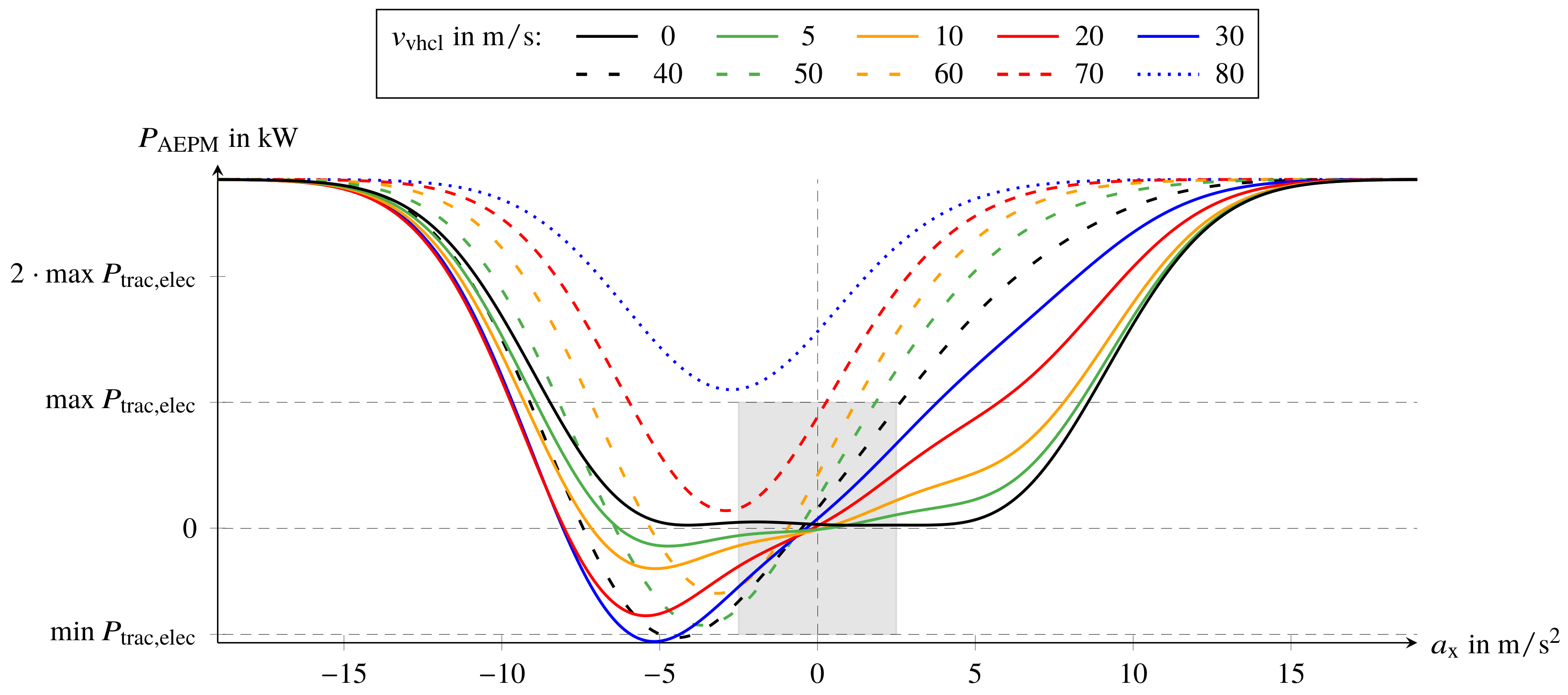
3.4. Adaptive Electrical Power Model

The AEPM answers the question of how much electrical traction power $P_{\mathrm{trac},\mathrm{elec}}$ is required for a specific combination of $v_{\mathrm{vhcl}}$ and $a_{\mathrm{x}}$. The ALC uses the AEPM for trajectory optimization in the trajectory module.

$P_{\mathrm{trac},\mathrm{elec}}$ is determined from measured voltages and currents at the electric motors that are available on the CAN bus. Apart from power train losses, $P_{\mathrm{trac},\mathrm{elec}}$ equals $P_{\mathrm{trac},\mathrm{mech}}$, which can be computed as the product of $F_{\mathrm{trac}}$ and $v_{\mathrm{vhcl}}$ (c.f. (6),(7)). According to Section 3.3 we can model $F_{\mathrm{trac}}$ as a function of $v_{\mathrm{vhcl}}$ and $a_{\mathrm{x}}$. Therefore the AEPM also has the inputs $v_{\mathrm{vhcl}}$ and $a_{\mathrm{x}}$:

$$P_{\mathrm{AEPM}}=\mathrm{AEPM}(v_{\mathrm{vhcl}},a_{\mathrm{x}}).$$

(12)

The model output $P_{\mathrm{AEPM}}$ includes aggregated power train losses that vary with respect to $v_{\mathrm{vhcl}}$ or $a_{\mathrm{x}}$.

A substantial fraction of $P_{\mathrm{trac},\mathrm{mech}}$ is needed to overcome the inertial force $m_{\mathrm{vhcl}}·{\dot{v}}_{\mathrm{vhcl},\mathrm{x}}$. The corresponding power $m_{\mathrm{vhcl}}·{\dot{v}}_{\mathrm{vhcl},\mathrm{x}}·v_{\mathrm{vhcl}}$ includes an unseparable product of ${\dot{v}}_{\mathrm{vhcl},\mathrm{x}}$ and $v_{\mathrm{vhcl}}$. For negligible road slope angle, $v_{\mathrm{vhcl}}$ and ${\dot{v}}_{\mathrm{vhcl},\mathrm{x}}$ coincide with the model inputs $v_{\mathrm{vhcl}}$ and $a_{\mathrm{x}}$ because of (9). Therefore the linear model structure used in Section 3.3 for the ATFM is not suitable for the AEPM.

Kernel methods apply a nonlinear transformation on the provided data in order to transform it into a high-dimensional feature space, in which the tranformed data is linearly separable. With most kernel-based methods the required memory increases with the number of processed data points. The AEPM is based on the Fixed-Budget Kernel Recursive Least-Squares (FBKRLS) algorithm [33,34]. FBKRLS keeps the required memory constant which enables online applications. As a result, the AEPM can learn a nonlinear mapping iteratively and track changes of vehicle parameters or power train properties over time.

In the AEPM, FBKRLS positions kernels in the $(v_{\mathrm{vhcl}},a_{\mathrm{x}})$ plane and computes a coefficient for each kernel. The model output $P_{\mathrm{AEPM}}$ for a specific $(v_{\mathrm{vhcl}},a_{\mathrm{x}})$ combination is the weighted sum of all kernels for this combination.

The trajectory optimization algorithm NRBA queries $(v_{\mathrm{vhcl}},a_{\mathrm{x}})$ combinations and takes decisions based on $P_{\mathrm{AEPM}}$. The output of the standard FBKRLS is zero for areas, in which no data points have occured yet. This property is undesired for trajectory optimization because it encourages NRBA to favor high velocities or accelerations that are beyond the capabilities of the vehicle. We train the AEPM with normalized and shifted data. With normalization of model inputs and outputs we achieve better aproximation quality. By shifting the desired output values we get large model outputs for $(v_{\mathrm{vhcl}},a_{\mathrm{x}})$ combinations that exceed the vehicles capabilities.

Figure 3 depicts the denormalized and backshifted model output $P_{\mathrm{AEPM}}$ as a function of $a_{\mathrm{x}}$ for various vehicle velocities. The shift produces a large crater which causes high power outputs of the AEPM for unreachable $(v_{\mathrm{vhcl}},a_{\mathrm{x}})$ combinations and hence NRBA avoids trajectories that lead to such combinations. For medium negative $a_{\mathrm{x}}$, the electrical traction power is negative, which indicates that power is recuperated into the HV battery.

3.5. Route Data Module

The input to the route data module is map data is provided by the navigation system via the CAN bus. The map data consists of six vectors that contain the values and corresponding positions of legal speed limits, road curvature and road slope for the road section ahead of the vehicle. Similar to a run-length encoding, the vectors contain only information for positions at which the corresponding quantity changes significantly. The route data module is executed every 500 ms and convertes the map data to a meter-discrete representation for up to 3 km ahead of the vehicle position The route data module returns three vectors that describe the courses of legal speed limit, road curvature and road slope. Furthermore, it provides information on whether the route data changed strongly compared to the previous call, e.g., because the driver took a different route at a junction than expected.

3.6. Trajectory Module

Inputs to the trajectory module are map data from the route data module, parameters of the AEPM provided by the parameter adaption module, vehicle data and the selected driving mode.

In Section 3.6.1 we state how we create an upper speed limit for the route ahead from map data followed by a definition of the velocity trajectory in Section 3.6.2. In driving mode “Normal” and driving mode “Sport” trajectory optimization, without consideration of electrical traction power, is performed as we describe in Section 3.6.3. In contrast, in driving mode “Range” we optimize the trajectory with additional respect to the electrical traction power as stated in Section 3.6.4. The enforcement of trajectory constraints is described in Section 3.6.5.

The trajectory module is called every 500 ms and then either continues planning the current trajectory or starts planning a new velocity trajectory. Continuing planning the current trajectory means that the module only performs additional iterations of the optimization algorithm using the same upper speed limit as before until it reaches the end of the upper speed limit or an iteration limit. In contrast, planning a new trajectory requires computation of a new upper speed limit first. Planning of a new trajectory occurs after a certain driven distance or time limit is exceeded, if the route data has changed strongly or if the vehicle velocity deviates strongly from the planned velocity. Outputs of the trajectory module are parameters of the velocity trajectory.

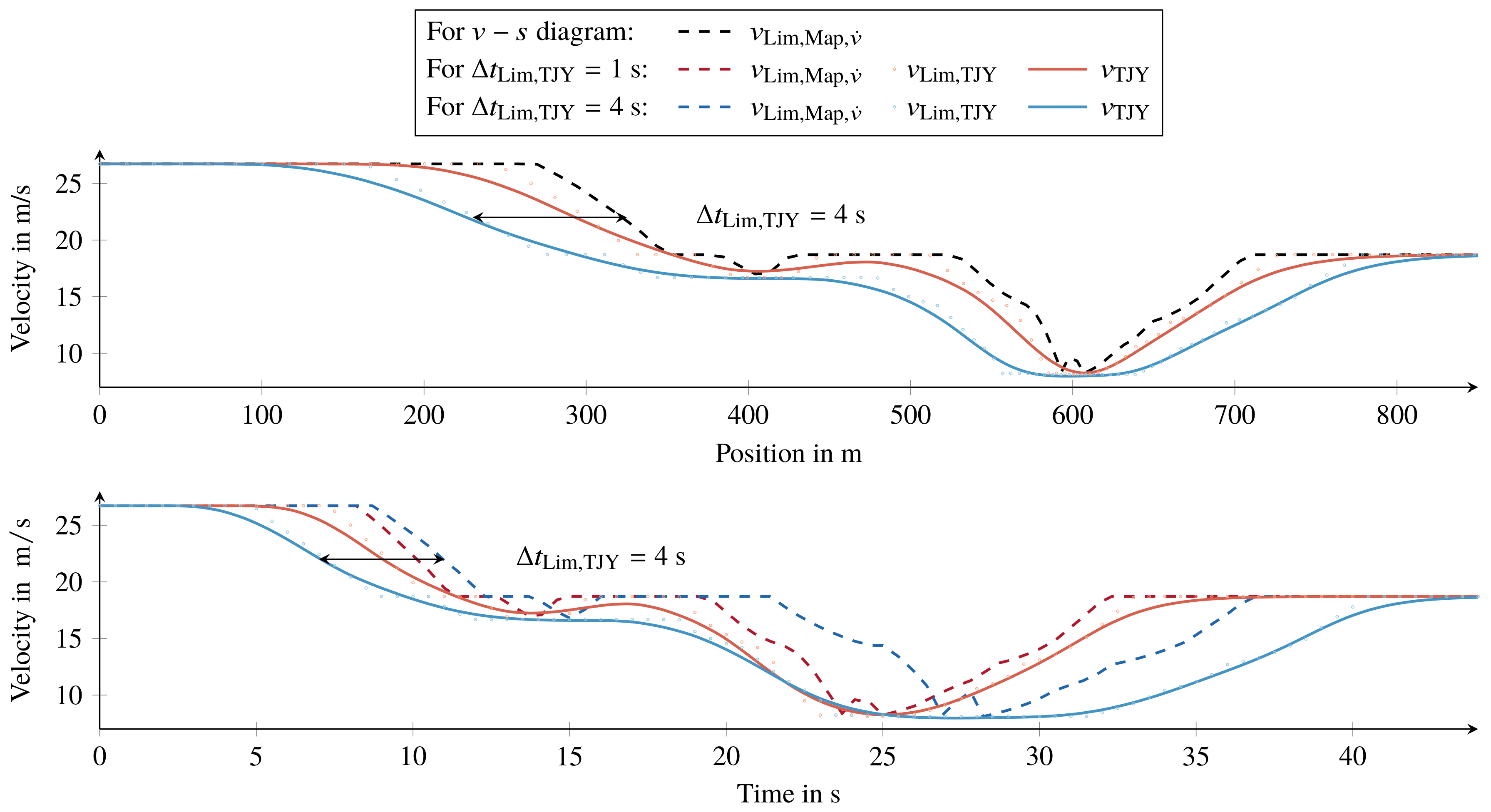
3.6.1. Generation of Upper Speed Limit

We compute an upper speed limit for each meter of the road section ahead of the vehicle from map data. The upper speed limit takes into account limitations of driving dynamics as well as safety and comfort requirements and serves as input data for the trajectory optimization.

The course of the legal speed limit forms the basis of the upper speed limit. On highway sections without a legal speed limit, we set the upper speed limit to a value that depends only on the selected driving mode and increases from mode “Range” via mode “Normal” to mode “Sport”. Thereby the vehicle velocity can vary between rather unhurried and rather fast on such sections. The upper speed limit is corrected down only if needed because of curves, crests, or comfort requirements.

Driving with vehicle velocity $v_{\mathrm{vhcl}}$ on a road with curvature c causes a lateral acceleration $a_{\mathrm{y}}$ with $a_{\mathrm{y}}=v_{\mathrm{vhcl}}^2·c$. A characteristic curve that describes a comfortable lateral acceleration as a function of vehicle velocity is stated in [35]. According to this characteristic curve, the lateral acceleration tolerated by a normal driver reaches its maximum of about $4\mathrm{m}/{\mathrm{s}}^2$ at around $55\mathrm{km}/\mathrm{h}$. We define three lateral acceleration look-up tables based on this characteristic curve, one for each driving mode. These are then used to limit the velocity in curves.

With road slope data we compute how far ahead we can see the road according to geometrical considerations and lower the maximum velocity if necessary to ensure that with maximum possible deceleration the vehicle can always come to a standstill within half of the visible road section ahead. In the last step we limit the variation of the course of velocity according to the desired positive and negative longitudinal acceleration. Hereby, the selected driving mode determines which longitudinal acceleration look-up table is used. The result is a set of P data points that describes the meter-discrete upper speed limit:

$$(s_p,v_{\mathrm{Lim},\mathrm{Map},\stackrel{.}{v},p}),s_p=p-1,p=1,2,\dots ,P$$

(13)

where s denotes the position measured from the vehicle position in driving direction and $v_{\mathrm{Lim},\mathrm{Map},\dot{v}}$ denotes the speed limit from map data with desired acceleration. The dashed line displayed in the upper diagram of Figure 4 is an example of such an upper speed limit.

3.6.2. Representation of Velocity Trajectory

We represent the trajectory velocity $v_{\mathrm{TJY}}$ using a B-spline function $v_{\mathrm{TJY}}\left(t\right)$ with respect to time t. The knot vector $\mathit{\kappa }$ and and function degree d define the number J of the basis functions b as well as their shape. Together with coefficient vector $\mathit{x}$ with

$$\mathit{x}={\left(x_1,\dots ,x_j,\dots ,x_J\right)}^{\top }$$

(14)

the B-spline function is fully defined. Its value is given by the sum of basis functions, each of which is weighted with its corresponding coefficient x:

$$v_{\mathrm{TJY}}\left(t\right)=\sum _{j=1}^J{b}_j(\mathit{\kappa },d,t)·x_j.$$

(15)

We use a cubic B-spline function, hence degree $d=3$. It is twice continously differentiable which means that the trajectory acceleration $a_{\mathrm{TJY}}$ and the trajectory jerk $j_{\mathrm{TJY}}$ are continuous. These quantities are the first and second derivative of $v_{\mathrm{TJY}}$. In our application, $\mathit{\kappa }$ has K equidistant and strictly monotonously increasing knots $\kappa$:

$$\mathit{\kappa }=({\kappa }_1,{\kappa }_2,\dots ,{\kappa }_K)=\left(-\Delta t_{\kappa }·d,\Delta t_{\kappa }·(d+1),\dots ,\Delta t_{\kappa }·d+K-1\right).$$

(16)

The parameter $\Delta t_{\kappa }$ denotes the constant temporal distance of neighboring knots. Due to the choice of $\mathit{\kappa }$, the trajectory can be evaluated for $t\ge 0$. For mathematical details concerning this function type and relevant formulas we refer to [5,19].

3.6.3. Trajectory Optimization

For adaption of $v_{\mathrm{TJY}}\left(t\right)$ to the upper speed limit, we solve the approximation problem

$$\widehat{\mathit{x}}=\underset{\mathit{x}}{arg\; min}\sum _{p=1}^P\left(R_v^{-1}·{\left[v_{\mathrm{Lim},\mathrm{TJY}}\left(s_{\mathrm{TJY}}\left(t_p\right)\right)-v_{\mathrm{TJY}}\left(t_p\right)\right]}^2\right.\left.+R_a^{-1}·a_{\mathrm{TJY}}{\left(t_p\right)}^2+R_j^{-1}·j_{\mathrm{TJY}}{\left(t_p\right)}^2\right),$$

(17)

whereby t is discretized using the constant temporal distance of neighboring data points $\Delta t_{\mathrm{It}}$:

$$t_p=(p-1)·\Delta t_{\mathrm{It}},p=1,\dots ,P.$$

(18)

The optimization problem includes a change of representation space from position to time in the first summand. The trajectory position $s_{\mathrm{TJY}}$ is measured from $t=0$, hence $s_{\mathrm{TJY}}(t=0)=0$, and calculated as stated in [36]. By penalizing deviations of $a_{\mathrm{TJY}}$ and $j_{\mathrm{TJY}}$ from zero, we stabilize the $v_{\mathrm{TJY}}\left(t\right)$ trajectory and avoid uncomfortable driving that can be caused by acceleration peaks and velocity oscillations.

Each of these optimization goals has a corresponding weight. $R_v^{-1}$ denotes the weight of velocity error square, $R_a^{-1}$ denotes the weight of acceleration error square, and $R_j^{-1}$ denotes the weight of jerk error square. $R_v^{-1}$ can be interpreted as a weight for low travel time whereas both $R_a^{-1}$ and $R_j^{-1}$ refer to driving comfort.

The goal of RBA and NRBA is to approximate data points [5,19]. However, the data points in (13) also present a constraint to $v_{\mathrm{TJY}}$. We take into account the constraint character by using in (17) the data set

$$(s_p,v_{\mathrm{Lim},\mathrm{TJY},\rho }),s_p=p-1,p=1,2,\dots ,P.$$

(19)

The speed limit for trajectory optimization $v_{\mathrm{Lim},\mathrm{TJY}}$ is derived from (13) and the minimum of $v_{\mathrm{Lim},\mathrm{Map},\dot{v}}$ within a spatial distance around $s_{\mathrm{TJY}}$:

$$\begin{array}{cc}\hfill v_{\mathrm{Lim},\mathrm{TJY}}& =min\left(v_{\mathrm{Lim},\mathrm{Map},\dot{v}}\left[p_{min}\right],\dots ,v_{\mathrm{Lim},\mathrm{Map},\dot{v}}\left[p_{max}\right]\right)\hfill \\ \hfill p_{min}& =\mathrm{round}\left(s_{\mathrm{TJY}}-v_{\mathrm{TJY}}·\Delta t_{\mathrm{Lim},\mathrm{TJY}}+1\right)\hfill \\ \hfill p_{max}& =\mathrm{round}\left(s_{\mathrm{TJY}}+v_{\mathrm{TJY}}·\Delta t_{\mathrm{Lim},\mathrm{TJY}}+1\right).\hfill \end{array}$$

(20)

This distance depends on $v_{\mathrm{TJY}}$ and the temporal safety margin to upper speed limit $\Delta t_{\mathrm{Lim},\mathrm{TJY}}$, which is a tuning parameter. In each iteration p of RBA or NRBA, we determine $s_{\mathrm{TJY}}$ for the current time $t_p$ by temporal integration of $v_{\mathrm{TJY}}$ with its currently estimated coefficient vector $\mathit{x}$ in order to calculate $v_{\mathrm{Lim},\mathrm{TJY}}$ for (17) with (20).

In (17) the coefficient vector $\mathit{x}$ is nonlinearly linked to the error $\left(v_{\mathrm{Lim},\mathrm{TJY}}\left(s_{\mathrm{TJY}}\right)-v_{\mathrm{TJY}}\right)$ by (19). This makes (17) a NWLS problem that we can solve with NRBA. With the described iterative approach, however, we approximate the NWLS problem (17) by a WLS problem such that RBA suffices. The advantage of RBA is that its computational effort is lower than that of NRBA. In a different context, [37,38] approximated a nonlinear problem by a quadratic problem in order to be able to apply a quadratic programming method instead of a sequential quadratic programming method like the Levenberg-Marquardt (LM) algorithm.

Figure 4 shows trajectory optimization examples using RBA. The Matlab source code is provided in [39]. The upper diagram depicts the velocity v versus the position s measured from the vehicle in driving direction. The $v-s$ diagram allows the comparison of different trajectories depicted by solid lines against the same upper speed limit $v_{\mathrm{Lim},\mathrm{Map},\dot{v}}$ depicted by a dashed line. In contrast, in the lower $v-t$ diagram we need to show the spatially defined upper speed limit for each trajectory separately.

The red trajectory results from $\Delta t_{\mathrm{Lim},\mathrm{TJY}}=1\mathrm{s}$, $\Delta t_{\mathit{\kappa }}=1\mathrm{s}$, $\Delta t_{\mathrm{It}}=0.1\mathrm{s}$ and $\left(I\right)=1$. The parameter I denotes the number of intervals of the B-spline function that are optimized simultaneously. RBA and NRBA can adapt $I+d$ neighboring coefficients in a single iteration [5,19].

The blue trajectory differs only in that $\Delta t_{\mathrm{Lim},\mathrm{TJY}}=4\mathrm{s}$. Dots indicate the $v_{\mathrm{Lim},\mathrm{TJY}}$ values that occur during the iterations of RBA. Only every tenth $v_{\mathrm{Lim},\mathrm{TJY}}$ point is shown.

The weighting combination reads $R_v^{-1}=\frac{1}{5},R_a^{-1}=\frac{1}{10},R_j^{-1}=1$ and will also be used in the remainder of this work. This combination was determined from trajectory optimization experiments. In data approximation experiments for RBA and NRBA performed in [5,19], the equivalent to $R_a^{-1}$ is ten and two times, respectively, larger and the equivalent to $R_j^{-1}$ is 1000 and 200 times, respectively, larger. This is because in these experiments the goal is to smooth jumps of an amplitude of ten in the data set. However, the velocity range of an upper speed limit is often much larger and unless $R_a^{-1}$ and $R_j^{-1}$ are strongly reduced, the trajectories do not follow the course of the upper speed limit. Furthermore, $R_v^{-1}$ is five times smaller than in the data approximation experiments to assign a higher relative weighting to $R_a^{-1}$ and $R_j^{-1}$, which are relevant for driving comfort.

In the $v-s$ diagram the $v_{\mathrm{Lim},\mathrm{TJY}}$ data points are less close at high velocities (e.g., for $s\le 200\mathrm{m}$) than at low velocities (e.g., at $s=600\mathrm{m}$). Furthermore, $\Delta t_{\mathrm{Lim},\mathrm{TJY}}$ causes that at high velocities the spatial distance between the courses of $v_{\mathrm{Lim},\mathrm{TJY}}$ and $v_{\mathrm{Lim},\mathrm{Map},\dot{v}}$ is larger. Provided that $\Delta t_{\mathrm{It}}$ is sufficiently small and that $\Delta t_{\mathrm{Lim},\mathrm{TJY}}$ is sufficiently large, there are enough data points to ensure that the resulting trajectory does not exceed $v_{\mathrm{Lim},\mathrm{Map},\dot{v}}$ noticeably at local minima, e.g., at $s=400\mathrm{m}$ and $s=600\mathrm{m}$.

Increasing $\Delta t_{\mathrm{Lim},\mathrm{TJY}}$ reduces short-lasting velocity peaks. For example, at $s=500\mathrm{m}$ $v_{\mathrm{Lim},\mathrm{Map},\dot{v}}$ has a local maximum that $v_{\mathrm{Lim},\mathrm{TJY}}$ with $\Delta t_{\mathrm{Lim},\mathrm{TJY}}=4\mathrm{s}$ cannot reflect. For $\Delta t_{\mathrm{Lim},\mathrm{TJY}}=1\mathrm{s}$, $v_{\mathrm{Lim},\mathrm{TJY}}$ has a local maximum as well but the corresponding trajectory does not closely follow $v_{\mathrm{Lim},\mathrm{TJY}}$. However, proximity to $v_{\mathrm{Lim},\mathrm{TJY}}$ not the primary goal because the course of $v_{\mathrm{Lim},\mathrm{TJY}}$ is not jerk-free and must be smoothed by the trajectory. The extent to which the trajectory can follow $v_{\mathrm{Lim},\mathrm{TJY}}$ is determined by the weighting factors $R_v^{-1}$, $R_a^{-1}$, $R_j^{-1}$ and the temporal distance of neighboring knots $\Delta t_{\kappa }$.

3.6.4. Trajectory Optimization with Consideration of Electrical Traction Power

For consideration of the required electrical power we augment (17) with the summand $R_P^{-1}·{\left(P_{\mathrm{AEPM}}\right)}^2$, which penalizes absolute values of $P_{\mathrm{AEPM}}$. $R_P^{-1}$ denotes the weight of the power error square:

$$\begin{array}{c}\hfill \widehat{\mathit{x}}=\underset{\mathit{x}}{arg\; min}\sum _{p=1}^P\left(R_v^{-1}·{\left[v_{\mathrm{Lim},\mathrm{TJY}}\left(s_{\mathrm{TJY}}\left(t_p\right)\right)-v_{\mathrm{TJY}}\left(t_p\right)\right]}^2\right.\\ \hfill \left.+R_a^{-1}·a_{\mathrm{TJY}}{\left(t_p\right)}^2+R_j^{-1}·j_{\mathrm{TJY}}{\left(t_p\right)}^2+R_P^{-1}·P_{\mathrm{AEPM}}{\left(t_p\right)}^2\right).\end{array}$$

(21)

The model output $P_{\mathrm{AEPM}}$ is given by

$$P_{\mathrm{AEPM}}\left(t\right)=\mathrm{AEPM}(v_{\mathrm{TJY}},a_{\mathrm{x}}).$$

(22)

The longitudinal specific acceleration $a_{\mathrm{x}}$ can be computed as

$$a_{\mathrm{x}}=a_{\mathrm{TJY}}+g·sin\left(\alpha \left(s_{\mathrm{TJY}}\right)\right)$$

(23)

and the road slope angle $\alpha$ can be derived from map data. As $P_{\mathrm{AEPM}}$ correlates with the product of $v_{\mathrm{TJY}}$ and its derivative $a_{\mathrm{TJY}}$, an approximation of this fourth optimization goal such that RBA can be applied is not promising for useful results. Therefore, we use NRBA, which includes a marginalized particle filter (MPF) [5].

Braking for an upcoming curve usually requires negative $P_{\mathrm{AEPM}}$ for recuperation. Strong penalization of $P_{\mathrm{AEPM}}^2$ can prevent braking for upcoming curves. In order to enable sufficient braking power, the computation of the error $e=\left(v_{\mathrm{Lim},\mathrm{TJY}}\left(s_{\mathrm{TJY}}\right)-v_{\mathrm{TJY}}\right)$ within the MPF is designed asymetrically. If $e\le 0$, we replace $v_{\mathrm{Lim},\mathrm{TJY}}$ with $v_{\mathrm{Lim},\mathrm{TJY}}=R_{\mathrm{v}>\mathrm{vLim}}·e+v_{\mathrm{TJY}}$. Hence, e is multiplied with $R_{\mathrm{v}>\mathrm{vLim}}=2$ if $v_{\mathrm{TJY}}>v_{\mathrm{Lim},\mathrm{TJY}}$. In the case of $e>0$ the original error e is multiplied with $R_{\mathrm{v}<\mathrm{vLim}}=1$, which is the error weighting for $v_{\mathrm{TJY}}<v_{\mathrm{Lim},\mathrm{TJY}}$. The reworked measurement reads $v_{\mathrm{Lim},\mathrm{TJY}}=R_{\mathrm{v}<\mathrm{vLim}}·e+v_{\mathrm{TJY}}$. In either case the resulting error square is then weighted with $R_v^{-1}$ in the MPF. In (17) the asymmetrical weighting of e is omitted because it has very limited influence. The reason is that there is no incentive to exceed $v_{\mathrm{Lim},\mathrm{Map},\dot{v}}$ because of the missing optimization goal regarding $P_{\mathrm{AEPM}}$.

Figure 5 depicts various quantities for trajectories determined by NRBA with $R_P^{-1}={10}^{-2}$, $R_P^{-1}={10}^{-3}$ and $R_P^{-1}={10}^{-4}$ versus the position. The Matlab source code is provided in [39] as well. For comparison, we also show a trajectory determined with the LM algorithm for $R_P^{-1}={10}^{-4}$. The remaining parameters are $\Delta t_{\kappa }=2\mathrm{s}$, $\Delta t_{\mathrm{It}}=0.25\mathrm{s}$, $\Delta t_{\mathrm{Lim},\mathrm{TJY}}=1\mathrm{s}$ and $I=1$. In the depicted situation we can compare the energy consumptions that result from following each of the trajectories because at $s=0\mathrm{m}$ and also at $s=2690\mathrm{m}$ the kinetic and potential energy of a vehicle does not differ with the trajectory that it tracks.

For $R_P^{-1}={10}^{-4}$, the NRBA and LM trajectories are similar and follow $v_{\mathrm{Lim},\mathrm{Map},\dot{v}}$ closely. With LM, the energy loss between HV battery and wheels $E_{\mathrm{Loss}}$ equals $77\mathrm{Wh}$ and the required HV battery energy $E_{\mathrm{Batt}}$ equals $721\mathrm{Wh}$. $E_{\mathrm{Loss}}$ and $E_{\mathrm{Batt}}$ result from a detailed power train model. For $R_P^{-1}={10}^{-4}$, NRBA achieves $E_{\mathrm{Loss}}=75\mathrm{Wh}$ and $E_{\mathrm{Batt}}=714\mathrm{Wh}$. When $R_P^{-1}$ is increased, peaks in the electrical traction power $P_{\mathrm{trac},\mathrm{elec}}$ are reduced which translates to lower $E_{\mathrm{Loss}}$ and $E_{\mathrm{Batt}}$. $R_P^{-1}={10}^{-3}$ leads to $E_{\mathrm{Loss}}=71\mathrm{Wh}$ and $E_{\mathrm{Batt}}=703\mathrm{Wh}$. For $R_P^{-1}={10}^{-2}$ $E_{\mathrm{Loss}}=65\mathrm{Wh}$ and $E_{\mathrm{Batt}}=684\mathrm{Wh}$ result.

Regarding the driving style we notice that for higher $R_P^{-1}$, the trajectories exhibit lower accelerations, stay more below $v_{\mathrm{Lim},\mathrm{Map},\dot{v}}$, avoid short-lasting velocity peaks and react more to the road slope, which affects $P_{\mathrm{trac},\mathrm{elec}}$. For example, consider the red trajectory for $R_P^{-1}={10}^{-2}$. Below 600 m, this trajectory strongly deviates from the upper speed limit because of the high slope. When the sign of the slope changes to negative at around 600 m, the red trajectory reduces this deviation to a large extent in a second and stronger acceleration phase. We also see that the red trajectory reflects the local maxima of the road slope at 1100 m and 1450 m.

Furthermore, a comparison of the trajectories indicates that the deviation from the upper speed limit is larger at a positive slope, e.g., between 800 m and 1400 m, than at a negative slope, e.g., between 1600 m and 2200 m.

3.6.5. Consideration of Additional Trajectory Constraints

The parameter projection method of [40] allows modification of the trajectory coefficients such that the trajectory fulfills certain constraints at certain points. We use this method to enforce that $v_{\mathrm{TJY}}$ and $a_{\mathrm{TJY}}$ of the new trajectory equal $v_{\mathrm{vhcl}}$ and ${\dot{v}}_{\mathrm{vhcl},\mathrm{x}}$, respectively, in two cases: First, if no valid previous trajectory is available, e.g., because map data was temporarily not available, and second, if $v_{\mathrm{vhcl}}$ deviates more than a threshold from $v_{\mathrm{TJY}}$, e.g., because the vehicle is at standstill. In all other cases we project $v_{\mathrm{TJY}}\left(t_1\right)$, $a_{\mathrm{TJY}}\left(t_1\right)$ and $j_{\mathrm{TJY}}\left(t_1\right)$ ($t_1=0$) of the new trajectory onto $v_{\mathrm{TJY}}$, $a_{\mathrm{TJY}}$ and $j_{\mathrm{TJY}}$ of the previous trajectory at its last evaluation point $t^{*}$ in order to achieve a twice continuously differentiable connection between both trajectories.

The parameter projection method changes only the parameter values that influence the trajectory function at $t_1$. If the trajectory is projected onto a vehicle at standstill and $\Delta t_{\kappa }$ is small, the trajectory will demand a very abrupt acceleration towards the upper speed limit. We get a comfortable velocity transition by choosing $R_a^{-1}$ initially high and reducing it linearly to its usual value during the first iterations.

The intelligent driver model (IDM) described in [41] provides an ACC functionality by calculating a target vehicle acceleration depending on the velocites of the own vehicle and vehicle ahead as well as the distance between them. With this target vehicle acceleration we can further modify $v_{\mathrm{Lim},\mathrm{TJY}}$ of (20) during the iterative solution of (17) such that the chosen time gap to the vehicle ahead is maintained.

3.7. Controller Module

Inputs to the controller module are the knot vector and estimated coefficient vector from the trajectory module as well as the estimated vehicle parameter vector from the parameter adaption module. Every $20\mathrm{ms}$ the controller modules computes $v_{\mathrm{TJY}}$ and $a_{\mathrm{TJY}}$ for the current point in time measured since beginning of last trajectory planning and translates these quantities into a motor torque demand $T_{\mathrm{des}}$.

Figure 6 depicts the controller module architecture and the control loop. $v_{\mathrm{TJY}}$, $a_{\mathrm{TJY}}$ and the road slope angle $\alpha$ are inputs to a pilot control and a model predictive control (MPC). The pilot control contains the ATFM and computes an open-loop torque demand $T_{\mathrm{des},\mathrm{PC}}$ with

$$T_{\mathrm{des},\mathrm{PC}}=\frac{F_{\mathrm{ATFM}}}{i_{\mathrm{G}}}·\frac{r_{\mathrm{dyn},\mathrm{FA}}+r_{\mathrm{dyn},\mathrm{RA}}}{2}$$

(24)

that causes the vehicle to roughly track $v_{\mathrm{TJY}}$ and $a_{\mathrm{TJY}}$. $i_{\mathrm{G}}$ is the gear ratio, $r_{\mathrm{dyn},\mathrm{FA}}$ the dynamic front axle tire radius and $r_{\mathrm{dyn},\mathrm{RA}}$ the dynamic rear axle tire radius. The traction force $F_{\mathrm{ATFM}}$ is determined by the ATFM according to (11), whereby we compute the vehicle motion vector ${\mathit{C}}_{\mathrm{Vhcl}}$ with

$${\mathit{C}}_{\mathrm{Vhcl}}:=(1,a_{\mathrm{x}},v_{\mathrm{TJY}}^2)$$

(25)

and determine $a_{\mathrm{x}}$ according to (23).

Due to imperfect map data, sensor data and ATFM, $v_{\mathrm{vhcl}}$ deviates from $v_{\mathrm{TJY}}$ and ${\dot{v}}_{\mathrm{vhcl},\mathrm{x}}$ from $a_{\mathrm{TJY}}$. The MPC computes a closed-loop torque demand $T_{\mathrm{des},\mathrm{MPC}}$ in order to minimize these deviations. In contrast to a proportional-integral-derivative (PID) controller, MPC can also take into account future set points which enables an anticipating look-ahead control. In our application, MPC consideres $v_{\mathrm{TJY}}$ and $a_{\mathrm{TJY}}$ for the current time step and nine future time steps.

The torque demand of the controller module $T_{\mathrm{des}}$ is the sum of $T_{\mathrm{des},\mathrm{PC}}$ and $T_{\mathrm{des},\mathrm{MPC}}$ and reaches the motor ECU via the CAN bus. The motor ECU distributes the torque demand among front motor and rear motor and controls these actuators accordingly. The control loop is closed through the vehicle.

4. Testing and Evaluation of the Automated Longitudinal Control

Section 4.1 details the reference route that we use for calibration and testing of the ALC in real test drives reported in Section 4.2, as well as for simulative investigations of the energy-saving potential of the ALC compared to drives with MLC described in Section 4.3.

4.1. Reference Route

The reference route is a roughly 23 km long round course on public roads through and around the village Weissach in Southwestern Germany, hence denoted Weissach round (WR). It comprises sections within villages as well as country roads. The legal speed limit varies between 30 km/h and 100 km/h and the road slope ranges from −10% to 10%. The WR is depicted in ([3], p. 96).

4.2. Test Drives and Acceptance Test

We conducted real test drives on the WR itself as well as on a highway and at roundabouts nearby. During these test drives we calibrated various ALC parameters in order to determine that the realized driving style fits the vehicle characteristics and the selected driving mode.

For the adaption of the lateral acceleration tables, we identified road sections with significant curvature in different velocity ranges. These were mainly roundabouts that can be passed at roughly $20\mathrm{km}/\mathrm{h}$, a roundabout with larger diameter than can be passed at about $50\mathrm{km}/\mathrm{h}$ and winding country roads with suitable velocities between $30\mathrm{km}/\mathrm{h}$ and $100\mathrm{km}/\mathrm{h}$. We drove each road section several times in repetition. In between, we evaluated whether the subjective impression fits the selected driving mode and adapted the position of the $(v$,$a_{\mathrm{y}})$ supporting points of the corresponding lateral acceleration table if neccessary.

For the longitudinal acceleration tables the approach was analogous. In addition to how the vehicle approaches and leaves roundabouts and sections with high curvature, sections of interest were transitions between the inside and outside of built-up areas as well as changes of the legal speed limit on the highway.

Concerning the weighting factors of the trajectory optimization and the MPC the goal was that no jerks are felt. For the MPC we especially considered hilly road sections and parameterized the MPC in such a way that while driving downhill with constant velocity, no uncomfortable alternation between propulsion and braking occurs.

In a final acceptance test about ten employees of the project partner who work in automotive research and development tested the ALC on self-chosen routes. The overall positive comments mentioned in particular, its comfortable and smooth driving style.

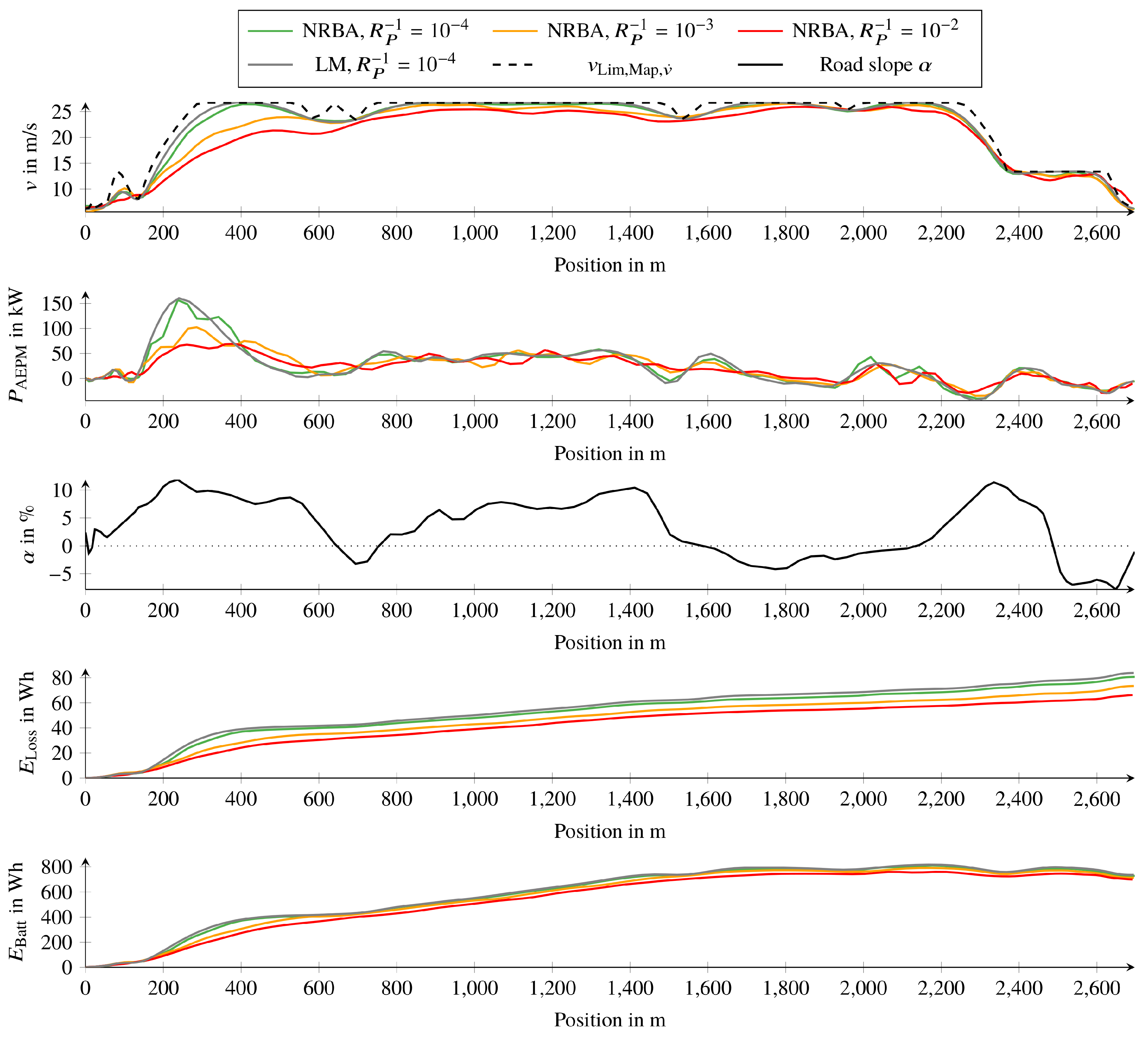
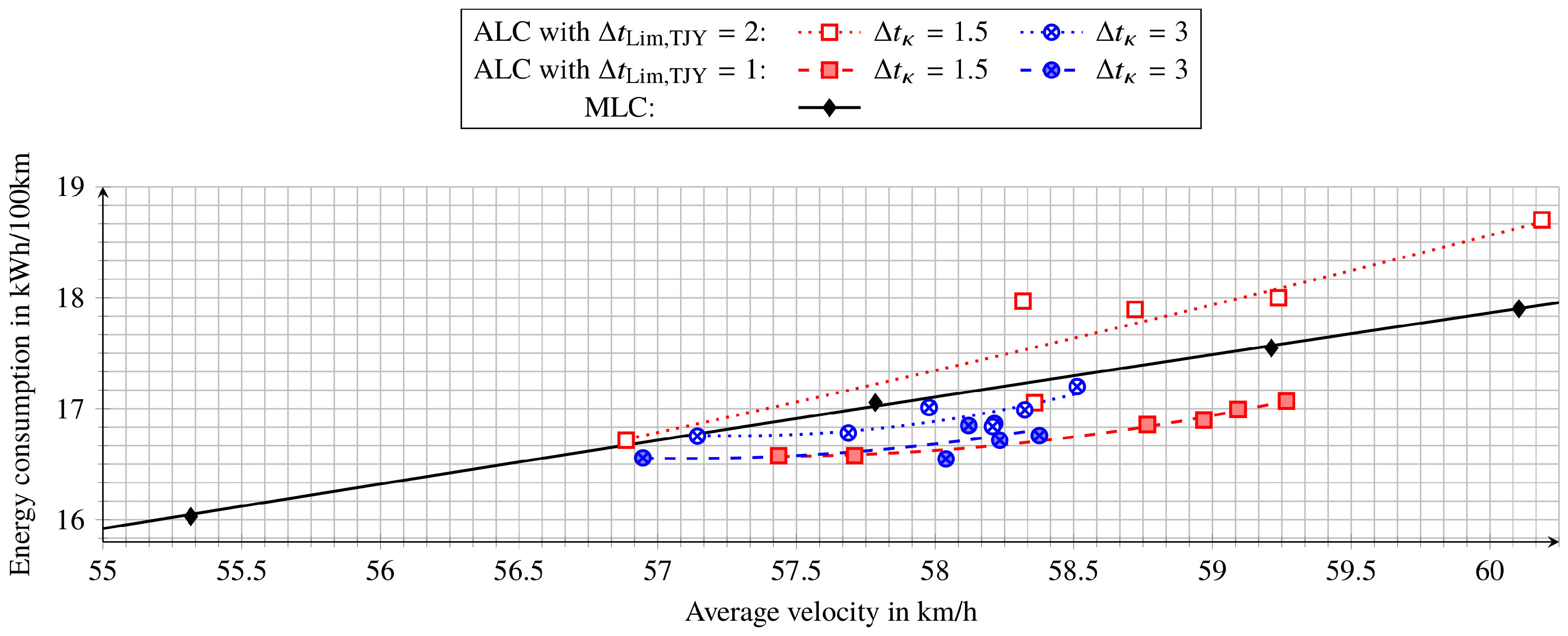
4.3. Energy-Saving Potential of Automated Longitudinal Control and Effects of Parameters

In simulations we investigate the energy-saving potential using the ALC with different parameter settings compared to drives with manual longitudinal control (MLC) on the WR.

The varied parameters are the temporal distance of neighboring knots $\Delta t_{\kappa }$, the temporal safety margin to upper speed limit $\Delta t_{\mathrm{Lim},\mathrm{TJY}}$ and the weight of power error square $R_P^{-1}$. Simulations of the ALC are conducted for all possible parameter combinations that result from $\Delta t_{\kappa }=\{1.5\mathrm{s},3\mathrm{s}\}$, $\Delta t_{\mathrm{Lim},\mathrm{TJY}}=\{1\mathrm{s},2\mathrm{s}\}$ and $R_P^{-1}=\{\frac{1}{10000},\frac{1}{5000},\frac{1}{1000},\frac{1}{500},\frac{1}{100},\frac{1}{50}\}$. The number of spline intervals I is set to one.

After each simulation, we convert the required trip time $t_{\mathrm{Trip}}$ for completing the WR into the average velocity by dividing $t_{\mathrm{Trip}}$ by the length of the WR and scale the energy consumption to the energy consumption per 100 km. This allows us to summarize each simulation result by a single data point in Figure 7.

Furthermore, we add a recorded real test drive on the WR with MLC to the comparison as a reference for the ALC results. In order to create multiple drives with MLC that differ in the average velocity, we multiply the recorded course of velocity with factors of about one. For a fair comparison between MLC and ALC, the course of velocity with MLC has to be adopted for the following reasons:

First, during the real test drive the driver had to stop the vehicle at junctions, react to other traffic participants and once during a short period the driver was restricted in the choice of vehicle velocity because of a preceding vehicle. Coming to a standstill and driving off again increases both the energy consumption and the required trip time. In order to not disadvantage MLC drives in the comparison, we adapt the recorded velocity with MLC to a typical ALC behavior in the mentioned situations.

Second, in curves the drives with MLC reach lateral acceleration absolute values larger than the maximum absolute value of lateral acceleration $a_{\mathrm{y},\max }$ allowed for the ALC. Increasing $a_{\mathrm{y},\max }$ leads to higher average velocity and less energy consumption. In order to compare ALC and MLC drives under the same conditions, we enforce the upper speed limit $v_{\mathrm{Lim},\mathrm{Map},\dot{v}}$ as an upper limit on the velocities of MLC drives. After these adaptions, we determine the energy consumption of drives with MLC using resimulation with a detailed vehicle model.

Figure 7 depicts the resulting data points for MLC and their quadratic approximation in black and by a solid line. This line serves as a benchmark for the ALC. The ALC data points should be below this line, meaning that the ALC achieves the same average velocity with less energy consumption or a higher average velocity for the same energy consumption.

Approximation lines for ALC data points indicate that average velocity and energy consumption increase when we reduce $\Delta t_{\kappa }$ from $3\mathrm{s}$ to $1.5\mathrm{s}$.

Lowering $\Delta t_{\mathrm{Lim},\mathrm{TJY}}$ increases the trajectory velocity at local minima of $v_{\mathrm{Lim},\mathrm{Map},\dot{v}}$. However, for $\Delta t_{\mathrm{Lim},\mathrm{TJY}}=1\mathrm{s}$ and $\Delta t_{\kappa }=3\mathrm{s}$ we did not yet observe that the trajectories exceed $v_{\mathrm{Lim},\mathrm{Map},\dot{v}}$ noticeably. See, for example, in Figure 5 the course of the trajectories that result for the same $\Delta t_{\mathrm{Lim},\mathrm{TJY}}$.

Furthermore, the approximation line for $\Delta t_{\mathrm{Lim},\mathrm{TJY}}=2\mathrm{s}$ and $\Delta t_{\kappa }=1.5\mathrm{s}$ comprises a larger range of average velocities and energy consumptions than the corresponding approximations for $\Delta t_{\kappa }=3\mathrm{s}$. The reason is that trajectories with larger $\Delta t_{\kappa }$ cannot follow the upper speed limit as closely because of the fewer degrees of freedom per time interval. Therefore the vehicle is generally slower and omits inefficient velocity peaks more frequently. As a result, there is less potential for an effect from varying weight $R_P^{-1}$.

With the parameter combination $\Delta t_{\mathrm{Lim},\mathrm{TJY}}=1\mathrm{s}$, $\Delta t_{\kappa }=1.5\mathrm{s}$ and $R_P^{-1}=\frac{1}{1000}$, the ALC achieves the largest energy savings with respect to MLC. At the same average velocity of $59.0\mathrm{km}/\mathrm{h}$, the ALC requires $3.4\%$ less energy than the MLC and with the same energy of $16.9\mathrm{kWh}/100\mathrm{km}$ the ALC achieves a $2.6\%$ higher average velocity. Increasing $R_P^{-1}$ from $\frac{1}{1000}$ to $\frac{1}{50}$ reduces the energy consumption by $2.9\%$ while the average velocity decreases by $3.1\%$.

For conventional vehicles the approach of [3,4] yields a reduction in energy consumption of 10% compared to MLC at the same average velocity. HEVs are investigated in [7]. A reduction of energy consumption by 11% only with optimization of energy management but without ALC is stated. For combined ALC and energy management optimization an 18 % reduction of energy consumption at the same average velocity is reported and an increase of average velocity by 21% for the same energy consumption.

In comparison, the savings achieved by the ALC in this work are much lower. However, they seem realistic because the power train of a BEV is more efficient in general and posseses less degrees of freedom for optimization. Furthermore, vehicles with conventional and hybrid power trains more frequently need to apply hydraulic brakes for deceleration. As hydraulic brakes dissipate kinetic energy, different driving styles are clearly reflected by the resulting energy consumption. In contrast, the hydraulic brakes of the research vehicle rarely need to be used because of the high recuperation capability of the vehicle. Therefore the effect of the driving style on the energy consumption is lower.

5. Conclusions

This publication presented a driver assistance system for energy-efficient automated longitudinal control (ALC) of a battery electric vehicle (BEV) and its evaluation in simulations and real test drives. The ALC for BEVs of the preceding research project [17,18] defines a spatial velocity trajectory using a cubic polynomial whereas the ALC proposed in this work uses a temporal trajectory defined by a B-spline function that allows for an arbitrary amount of degrees of freedom. Therefore the presented ALC enables planning of very long trajectories that define a much more dynamic vehicle behavior, especially at low velocities. Furthermore, the ALC of this work considers the required electrical traction power explicitly, and allows optimization of the trajectory, not only with respect to travel time and driving comfort, but also with respect to energy consumption.

The proposed ALC includes a novel trajectory optimization approach that falls into the category of direct methods (DM). In contrast to most other DM, of which the effort grows exponentially, its effort grows only linearly. We achieve this substantial saving by taking advantage of the simple BEV power train that allows to formulate constraints as soft constraints. The resulting unconstrained optimization problem can be solved using iterative filter-based data approximation algorithms.

Sometimes DM are also combined with dynamic programming for trajectory optimization because of their complementary properties ([2], p. 1430). In such cases the proposed optimization approach can also be applied to vehicles other than BEV and provide benefits concerning computational effort.

The energy-saving potential of the ALC for a BEV was investigated in simulations. On a chosen reference route, the BEV needs up to $3.4\%$ less energy with ALC than with manual longitudinal control at the same average velocity and achieves a $2.6\%$ higher average velocity at the same energy consumption. The proposed ALC can be used on its own or in combination with other driver assistance systems such as an automated lateral control and thereby contribute to automated driving of BEVs.

References

1. Dia, H.; Javanshour, F. Autonomous Shared Mobility-On-Demand: Melbourne Pilot Simulation Study. Transp. Res. Procedia 2017, 22, 285–296. [Google Scholar] [CrossRef]
2. Winner, H.; Hakuli, S.; Lotz, F.; Singer, C. Handbook of Driver Assistance Systems-Basic Information, Components and Systems for Active Safety and Comfort; Springer: Cham, Switzerland, 2016. [Google Scholar] [CrossRef]
3. Radke, T. Energieoptimale Längsführung von Kraftfahrzeugen durch Einsatz vorausschauender Fahrstrategien. Ph.D. Thesis, Karlsruhe Institute of Technology, Karlsruhe, Germany, 2013. [Google Scholar] [CrossRef]
4. Markschläger, P.; Wahl, H.G.; Weberbauer, F.; Lederer, M. Assistenzsystem für mehr Kraftstoffeffizienz. In Vernetztes Automobil: Sicherheit–Car-IT–Konzepte; Springer Fachmedien Wiesbaden: Wiesbaden, Germany, 2014; pp. 146–153. [Google Scholar] [CrossRef]
5. Jauch, J.; Bleimund, F.; Frey, M.; Gauterin, F. An Iterative Method Based on the Marginalized Particle Filter for Nonlinear B-Spline Data Approximation and Trajectory Optimization. Mathematics 2019, 7, 355. [Google Scholar] [CrossRef]
6. Passenberg, B. Theory and Algorithms for Indirect Methods in Optimal Control of Hybrid Systems. Ph.D. Thesis, Technische Universität München, München, Germany, 2012. [Google Scholar]
7. Wahl, H.G. Optimale Regelung eines prädiktiven Energiemanagements von Hybridfahrzeugen. Ph.D. Thesis, Karlsruhe Institute of Technology, Karlsruhe, Germany, 2015. [Google Scholar] [CrossRef]
8. Zhang, S.; Xiong, R. Adaptive energy management of a plug-in hybrid electric vehicle based on driving pattern recognition and dynamic programming. Appl. Energy 2015, 155, 68–78. [Google Scholar] [CrossRef]
9. Wu, D.; Li, Y.; Du, C.; Ding, H.; Li, Y.; Yang, X.; Lu, X. Fast velocity trajectory planning and control algorithm of intelligent 4WD electric vehicle for energy saving using time-based MPC. IET Intell. Transp. Syst. 2019, 13, 153–159. [Google Scholar] [CrossRef]
10. Van Keulen, T.; Naus, G.; de Jager, B.; van de Molengraft, R.; Steinbuch, M.; Aneke, E. Predictive Cruise Control in Hybrid Electric Vehicles. World Electr. Veh. J. 2009, 3, 494–504. [Google Scholar] [CrossRef] [Green Version]
11. Zhang, S.; Luo, Y.; Li, K.; Li, V. Real-Time Energy-Efficient Control for Fully Electric Vehicles Based on an Explicit Model Predictive Control Method. IEEE Trans. Veh. Technol. 2018, 67, 4693–4701. [Google Scholar] [CrossRef]
12. Han, J.; Kum, D.; Park, Y. Sensitivity analysis for assessing robustness of position-based predictive energy management strategy for fuel cell hybrid electric vehicle. World Electr. Veh. J. 2015, 7, 330–341. [Google Scholar] [CrossRef] [Green Version]
13. Kim, B.; Kim, Y.G.; Kim, T.; Park, Y.I.; Cha, S.W. HEV Cruise Control Strategy on GPS (Navigation) Information. World Electr. Veh. J. 2009, 3, 589–596. [Google Scholar] [CrossRef] [Green Version]
14. Lu, C.; Gong, J.; Lv, C.; Chen, X.; Cao, D.; Chen, Y. A Personalized Behavior Learning System for Human-Like Longitudinal Speed Control of Autonomous Vehicles. Sensors 2019, 19, 3672. [Google Scholar] [CrossRef] [PubMed]
15. Lv, C.; Hu, X.; Sangiovanni-Vincentelli, A.; Li, Y.; Martinez, C.M.; Cao, D. Driving-Style-Based Codesign Optimization of an Automated Electric Vehicle: A Cyber-Physical System Approach. IEEE Trans. Ind. Electr. 2019, 66, 2965–2975. [Google Scholar] [CrossRef]
16. González, D.; Pérez, J.; Milanés, V.; Nashashibi, F. A Review of Motion Planning Techniques for Automated Vehicles. IEEE Trans. Intell. Transp. Syst. 2016, 17, 1135–1145. [Google Scholar] [CrossRef]
17. Bleimund, F.; Dörr, D.; Fath, B.; Frey, M. Verbundprojekt “Schlüsseltechnologien für die nächste Generation der Elektrofahrzeuge (e-generation)”: Teilvorhaben KIT: “Assistenzsysteme für effizienten Energieeinsatz bei Elektrofahrzeugen”: Schlussbericht: Laufzeit des Vorhabens: 01.02.2012–31.12.2014; Technical Report; Karlsruher Institut für Technologie, Institut für Fahrzeugsystemtechnik, Lehrstuhl für Fahrzeugtechnik: Karlsruhe, Germany, 2015. [Google Scholar] [CrossRef]
18. Bleimund, F.; Rhode, S. Method, Computer Program Product, Device, and Vehicle for Calculating an Actuation Variable for the Operation of a Vehicle. German Patent EP2886409 (A1), 2015. [Google Scholar]
19. Jauch, J.; Bleimund, F.; Rhode, S.; Gauterin, F. Recursive B-spline approximation using the Kalman filter. Eng. Sci. Technol. Int. J. 2017, 20, 28–34. [Google Scholar] [CrossRef] [Green Version]
20. Bargende, M.; Reuss, H.; Wiedemann, J. In Proceedings of the 14 Internationales Stuttgarter Symposium: Automobil- und Motorentechnik; Springer Fachmedien Wiesbaden: Wiesbaden, Germany, 2014; pp. 19–29.
21. Bender, S.; Chodura, H.; Groß, M.; Kühn, T.; Watteroth, V. e-generation—Ein Forschungsprojekt mit positiver Bilanz. Porsche Eng. Magazin 2015, 2, 22–27, Accessed 04/28/2018, 18:24. [Google Scholar]
22. Zimmer, M. Durchgängiger Simulationsprozess zur Effizienzsteigerung und Reifegraderhöhung von Konzeptbewertungen in der Frühen Phase der Produktentstehung; Wissenschaftliche Reihe Fahrzeugtechnik Universität Stuttgart, Springer Fachmedien Wiesbaden: Wiesbaden, Germany, 2015; pp. 115–130. [Google Scholar]
23. Braess, H.; Seiffert, U. Vieweg Handbuch Kraftfahrzeugtechnik; ATZ/MTZ-Fachbuch, Springer Fachmedien Wiesbaden: Wiesbaden, Germany, 2013. [Google Scholar]
24. Schramm, D.; Hiller, M.; Bardini, R. Vehicle Dynamics—Modeling and Simulation; Springer: Berlin/Heidelberg, Germany, 2018. [Google Scholar] [CrossRef]
25. Guzzella, L.; Sciarretta, A. Vehicle Propulsion Systems: Introduction to Modeling and Optimization, 3rd ed.; Springer: Berlin, Germany, 2013. [Google Scholar]
26. Vaillant, M. Design Space Exploration zur multikriteriellen Optimierung elektrischer Sportwagenantriebsstränge. Ph.D. Thesis, Karlsruhe Institute of Technology, Karlsruhe, Germany, 2016. [Google Scholar] [CrossRef]
27. Qi, Z. Advances on air conditioning and heat pump system in electric vehicles—A review. Renew. Sustain. Energy Rev. 2014, 38, 754–764. [Google Scholar] [CrossRef]
28. Rhode, S.; Bleimund, F.; Gauterin, F. Recursive Generalized Total Least Squares with Noise Covariance Estimation. IFAC Proc. Volumes 2014, 47, 4637–4643. [Google Scholar] [CrossRef] [Green Version]
29. Ricciardi, V.; Acosta, M.; Augsburg, K.; Kanarachos, S.; Ivanov, V. Robust Brake Linings Friction Coefficient Estimation For Enhancement of EHB Control. In Proceedings of the 2017 XXVI International Conference on Information, Communication and Automation Technologies (ICAT), Sarajevo, Bosnia and Herzegovina, 26–28 October 2017; pp. 1–7. [Google Scholar] [CrossRef]
30. Zhou, M.; Jin, H.; Wang, W. A review of vehicle fuel consumption models to evaluate eco-driving and eco-routing. Transp. Res. Part D 2016, 49, 203–218. [Google Scholar] [CrossRef]
31. Rhode, S.; Hong, S.; Hedrick, J.K.; Gauterin, F. Vehicle tractive force prediction with robust and windup-stable Kalman filters. Control Eng. Pract. 2016, 46, 37–50. [Google Scholar] [CrossRef]
32. Stenlund, B.; Gustafsson, F. Avoiding windup in recursive parameter estimation. Prepr. Reglermöte 2002, 148–153. Available online: http://users.isy.liu.se/en/rt/fredrik/reports/02reglermoteakf.pdf (accessed on 10 July 2018).
33. Van Vaerenbergh, S.; Santamaria, I.; Liu, W.; Principe, J.C. Fixed-Budget Kernel Recursive Least-Squares. In Proceedings of the IEEE International Conference on Acoustics, Speech, and Signal Processing (ICASSP 2010), Dallas, TX, USA, 15–19 March 2010. [Google Scholar]
34. Van Vaerenbergh, S.; Santamaría, I. A Comparative Study of Kernel Adaptive Filtering Algorithms. In Proceedings of the 2013 IEEE Digital Signal Processing (DSP) Workshop and IEEE Signal Processing Education (SPE), Napa, CA, USA, 11–14 August 2013. [Google Scholar] [CrossRef]
35. Schimmelpfennig, K.-H.; Hebing, N. Geschwindigkeiten bei kreisförmiger Kurvenfahrt/Stabilitäts- und Sicherheitsgrenze. Der Verkehrsunfall 1982, 20, 97–99. [Google Scholar]
36. Sherar, P.A. Variational Based Analysis and Modelling Using B-splines. Ph.D. Thesis, Cranfield University, Cranfield, UK, 2003. [Google Scholar]
37. Carvalho, A.; Gao, Y.; Gray, A.; Tseng, E.; Borrelli, F. Predictive control of an autonomous ground vehicle using an iterative linearization approach. In Proceedings of the IEEE Conference on Intelligent Transportation Systems, ITSC, Hague, The Netherlands, 6–9 October 2013; pp. 2335–2340. [Google Scholar]
38. Falcone, P.; Tufo, M.; Borrelli, F.; Asgari, J.; Tseng, H.E. A linear time varying model predictive control approach to the integrated vehicle dynamics control problem in autonomous systems. In Proceedings of the 2007 46th IEEE Conference on Decision and Control, New Orleans, LA, USA, 12–14 December 2007; pp. 2980–2985. [Google Scholar] [CrossRef]
39. Jauch, J. ALC Matlab Files. 2019. Available online: http://github.com/JensJauch/ALC/releases (accessed on 14 July 2019). [CrossRef]
40. Simon, D. Kalman filtering with state constraints: A survey of linear and nonlinear algorithms. Control Theory Appl. IET 2010, 4, 1303–1318. [Google Scholar] [CrossRef]
41. Treiber, M.; Hennecke, A.; Helbing, D. Congested traffic states in empirical observations and microscopic simulations. Phys. Rev. E 2000, 62, 1805–1824. [Google Scholar] [CrossRef] [PubMed] [Green Version]
Figure 1. Power loss between HV battery and wheels P Loss versus electrical traction power P trac , elec for various combinations of vehicle velocity v vhcl and vehicle longitudinal acceleration v ˙ vhcl , x .
Wevj 10 00052 g001
Figure 2. System architecture of the automated longitudinal control.
Wevj 10 00052 g002
Figure 3. Electrical traction power P AEPM according to the adaptive electrical power model (AEPM) depending on longitudinal specific acceleration a x for various vehicle velocities v vhcl . The gray shaded area is the operating area of the ALC, max P trac , elec the maximum traction power and min P trac , elec the maximum recuperation power.
Wevj 10 00052 g003
Figure 4. Influence of temporal safety margin to upper speed limit Δ t Lim , TJY on speed limit for trajectory optimization v Lim , TJY and trajectory velocity v TJY . Only a subset of v Lim , TJY is shown. Upper diagram: The speed limit from map data with desired acceleration v Lim , Map , v ˙ is identical for both trajectories. Lower diagram: v Lim , Map , v ˙ differs with the trajectories.
Wevj 10 00052 g004
Figure 5. Velocity v, electrical traction power P AEPM according to adaptive electrical power model (AEPM), road slope α , energy loss between HV battery and wheels E Loss and HV battery energy E Batt for trajectories determined by nonlinear recursive B-spline approximation (NRBA) and Levenberg-Marquardt (LM) algorithm that differ in the weight of power error square R P 1 .
Wevj 10 00052 g005
Figure 6. Architecture of controller module and control loop. The trajectory velocity v TJY and trajectory acceleration a TJY are derived from the trajectory function. The pilot control based on the adaptive traction force model (ATFM) generates an open-loop motor torque demand T des , PC using v TJY , a TJY and the road slope angle α . The model predictive control (MPC) computes a closed-loop torque demand T des , MPC in order to minimize the remaining deviation of vehicle velocity v vhcl and vehicle longitudinal acceleration v ˙ vhcl , x from the desired values.
Wevj 10 00052 g006
Figure 7. Energy consumption versus average velocity on the reference route Weissach round with automated longitudinal control (ALC) under different parameter settings in comparison to adapted and resimulated real drives with manual longitudinal control (MLC).
Wevj 10 00052 g007