Robust Synthetic Data Generation for Sequential Financial Models Using Hybrid Variational Autoencoder–Markov Chain Monte Carlo Architectures

Abstract

Generating high-quality synthetic data is essential for advancing machine learning applications in financial time series, where data scarcity and privacy concerns often pose significant challenges. This study proposes a novel hybrid architecture that combines variational autoencoders (VAEs) with Markov Chain Monte Carlo (MCMC) sampling to enhance the generation of robust synthetic sequential data. The model leverages Gated Recurrent Unit (GRU) layers for capturing long-term temporal dependencies and MCMC sampling for effective latent space exploration, ensuring high variability and accuracy. Experimental evaluations on datasets of Google, Tesla, and Nestlé stock prices demonstrate the model’s superior performance in preserving statistical and temporal patterns, as validated by quantitative metrics (discriminative and predictive scores), statistical tests (Kolmogorov–Smirnov), and t-Distributed Stochastic Neighbour Embedding (t-SNE) visualisations. The experiments reveal the model’s scalability, maintaining high fidelity even under augmented dataset sizes and missing data scenarios. These findings position the proposed framework as a computationally efficient and structurally simple alternative to Generative Adversarial Network (GAN)-based methods, suitable for real-world applications in data-driven financial modelling.

1. Introduction

In 2006, Clive Humby coined the slogan ‘Data are the new Oil’ (https://futurescot.com/why-data-is-the-new-oil/ accessed on 4 July 2024), emphasizing data’s growing importance. Over time, data have become a critical resource, shaping industries and society. Advances in the digital world have transformed how data are generated, managed, and analysed, fostering new business practices and professional roles in data science and mining [1,2]; however, as noted by Floridi, the ethical governance and equitable application of data remain essential [3].

The evolution of data management began with relational databases in the 1980s, progressing to data warehouses (DWHs) in the 1990s, which aggregate and analyse large volumes of data, supporting strategic business decisions through Business Intelligence (BI). Schemas like star (denormalised for speed) and snowflake (normalised for reduced redundancy) optimise these analyses [4].

The emergence of Big Data, characterised by volume, velocity, variety, veracity, and variability, has further revolutionised data management; similarly, technologies such as the Hadoop, Apache Spark, and NoSQL databases are essential for handling Big Data, addressing challenges such as data quality, scarcity, privacy concerns, and ethical implications [5].

One promising solution to these challenges is synthetic data, which are generated using algorithms to simulate real datasets and mitigate scarcity, privacy, and class imbalance issues, with applications spanning finance, healthcare, artificial intelligence (AI), natural language processing, and education. It enables broader analyses and facilitates AI, computer vision, and speech synthesis advancements without compromising data security [6].

Despite these advancements, the generation of high-quality synthetic data remains an open challenge, particularly in maintaining fidelity to real-world data while ensuring diversity and robustness. This work addresses these challenges by proposing novel methodologies that enhance synthetic data generation through advanced modelling techniques. Specifically, the key contributions of this work are as follows:

• Enhanced Temporal Modelling: The Gated Recurrent Unit (GRU)-based architecture effectively captures long-term dependencies, enabling more accurate synthetic data generation compared to convolutional approaches.
• Improved Latent Space Sampling: Markov Chain Monte Carlo (MCMC) sampling enriches latent space exploration, ensuring variability and reducing divergence between real and synthetic data.
• Robustness and Scalability: The model demonstrates resilience to missing data and scalability in data augmentation tasks, maintaining performance across diverse conditions.

These contributions advance the understanding of synthetic data generation, addressing critical gaps in scalability, robustness, and representational fidelity.

The remainder of this article is structured as follows. Section 2 reviews the state of the art, while Section 3 provides the theoretical background. Section 4 discusses the model, while the experiments are presented in Section 5 and Section 6, respectively. A general discussion reviews the strengths and the limitations of this article in Section 7. Finally, Section 8 concludes the work, outlining directions for future research.

2. Related Work

The field of synthetic data generation has experienced significant growth, driven by advancements in algorithms and increasing demands across various domains. While early research focused heavily on natural language processing (NLP) with tools like ChatGPT and BARD [7], financial markets have emerged as a critical application area. Within this sector, machine learning models, particularly those dealing with sequential data, often require large, high-quality datasets to mitigate issues like imbalance and low signal-to-noise ratios. Synthetic data generation has proven essential in addressing these challenges, enabling improved predictive accuracy for tasks such as fraud detection and credit risk assessment [8]. This section explores state-of-the-art methods for synthetic data generation, focusing on financial applications and their capacity to manage the complexities of sequential data.

A Quantum Wasserstein Generative Adversarial Network with Gradient Penalty (QWGAN-GP) [9] is used to enhance financial time series prediction by generating synthetic data that replicate the statistical characteristics of the S&P 500 index. Leveraging a quantum generator and a classical discriminator, the approach effectively addresses limitations in financial datasets, such as insufficient representation of rare market events. The synthetic data generated were evaluated using metrics like Wasserstein distance and Dynamic Time Warping, showcasing high fidelity to the original data. Integrating these synthetic datasets into long short-term memory (LSTM) prediction models significantly improved the forecasting of general trends and extreme market events.

Monte Carlo methods have long been valued for their flexibility in simulating stochastic processes. Among recent advancements is the fintech-kMC model, which employs continuous-time Monte Carlo techniques to simulate customer behaviour on financial platforms [10]. This model excels in detecting potential bugs in machine learning processes while maintaining simplicity in implementation. Unlike traditional generative models that depend on high-quality data pipelines, kMC dynamically adjusts time steps based on event probabilities, ensuring realistic simulations.

Both static and dynamic rates are incorporated in kMC, allowing for diverse agent behaviours. Additionally, the introduction of agent archetypes ensures the simulation reflects varied customer actions. Despite its strengths, fintech-kMC has limitations, including its reliance on user-defined probability distributions and its reduced scalability for large-scale systems. Nevertheless, the approach effectively bridges the gap between realism and control in synthetic data generation for financial applications.

TimeGAN represents a significant advancement in the generation of sequential data by integrating temporal dynamics into Generative Adversarial Network (GAN) architectures. Unlike traditional GANs, which struggle with multivariate time series, TimeGAN combines autoregressive components, embedding networks, and adversarial training to learn both feature representations and temporal correlations [11]. This dual learning process enables the model to generate high-quality synthetic data that closely mimic the original sequences.

Evaluations of TimeGAN using metrics like diversity, fidelity, and predictive performance have shown its superiority over earlier methods such as the Recurrent Conditional GAN (RCGAN) and Continuous Recurrent Neural Network GAN (C-RNN-GAN). For example, TimeGAN demonstrates nearly perfect alignment between real and synthetic distributions, as evidenced by t-Distributed Stochastic Neighbour Embedding (t-SNE) and Principal Component Analysis (PCA) visualisations. Additionally, its predictive scores, tested on datasets like stock prices and energy consumption, are comparable to those achieved using real data, solidifying its effectiveness for real-world applications.

A real-world time series GAN (RTSGAN) extends the capabilities of GANs by addressing challenges like variable-length sequences and missing data [12]. It leverages an autoencoder to map sequences into a fixed-dimensional latent space, simplifying the generation process while preserving temporal dependencies. The framework employs a Wasserstein GAN (WGAN) for robust synthetic data generation and introduces RTSGAN-M for datasets with significant missing values.

Evaluations of RTSGAN on datasets such as energy usage and stock prices show its ability to outperform benchmarks like TimeGAN and Causal Optimal Transport GAN (COTGAN) in both discriminative and predictive tasks. The method’s flexibility makes it particularly suited for complex real-world scenarios, where incomplete data often pose significant challenges.

TimeVAE introduces a variational autoencoder (VAE) framework specifically designed for time-series data, emphasizing interpretability and reduced training complexity compared to GAN-based methods [13]. By combining convolutional and dense layers with a probabilistic latent space, TimeVAE generates synthetic data that closely align with real distributions.

The model’s evaluation demonstrates its strength in capturing temporal patterns, particularly for datasets with sinusoidal and structured sequences. TimeVAE’s simplicity and efficiency make it an attractive option for applications requiring fast, high-quality data generation, although its performance may decline with highly volatile data.

The VAE-GAN architecture merges the strengths of VAEs and GANs to address limitations like mode collapse and data diversity [14]. The VAE component encodes input data into a latent space, while the GAN generator uses this representation to create synthetic samples. This approach allows VAE-GAN to generate more representative data distributions without extensive preprocessing or domain knowledge.

VAE-GAN has been successfully applied to datasets related to energy and solar production, demonstrating superior performance in metrics like Kullback–Leibler divergence and Wasserstein distance compared to standalone GANs. Its ability to synthesize diverse and realistic data highlights its potential for applications in fields requiring robust and flexible data generation.

The models discussed offer varied strengths and limitations depending on the application. Monte Carlo methods like fintech-kMC excel in simplicity and control but may lack scalability for large datasets. TimeGAN and RTSGAN address the complexities of temporal data with advanced architectures, while TimeVAE provides a more interpretable and efficient alternative. VAE-GAN offers a hybrid approach, balancing diversity and representational accuracy.

Table 1. Summary of the discussed models.

Algorithm Name	Model Basis	Strenghts	Limitations
Fintech-kMC	Monte Carlo	Tailored for financial context; simple to implement	Limited scalability; less faithful to original data
TimeGAN	GAN	Captures temporal dynamics; robust across data types	High training complexity; requires extensive data
RTSGAN	GAN	Handles missing data; simplifies latent space	Computationally intensive; requires hyperparameter tuning
TimeVAE	VAE	Fast training; high interpretability	Limited handling of volatile data
VAE-GAN	GAN and VAE	Balances diversity and accuracy; flexible	High computational cost; potential mode collapse

summarises the comparative advantages and drawbacks of these models.

3. Background

The growing demand for synthetic data across industries has spurred the emergence of companies providing tailored solutions. Notable organisations like ‘Gretel.ai’, ‘Hazy’, and ‘MOSTLY AI’ focus on structured and unstructured synthetic data generation. These companies employ a variety of methods, including advanced statistical models and deep learning architectures, to address specific applications such as NLP and computer vision (https://mostly.ai/blog/synthetic-data-companies accessed on 4 January 2025). For instance, ‘Gretel.ai’ offers models like DoppelGANger (DGAN) and LSTM, while ‘Hazy’ uses DGAN, Synthetic Data Vault (SDV), and Bayesian models (https://hazy.com/docs/models accessed on 4 January 2025). Similarly, ‘Datacebo’ provides tools like DeepEcho and SDV, specifically designed for time-series data (https://sdv.dev/ accessed on 4 January 2025).

These diverse approaches allow organisations to tackle challenges in various domains, balancing accuracy, scalability, and complexity.

Naive Bayesian models are foundational statistical techniques that belong to the family of generative classifiers. They operate by applying Bayes’ theorem to compute posterior probabilities, assuming conditional independence among features. Despite their simplicity and restrictive assumptions, Naive Bayes models are effective, particularly in scenarios with small sample sizes or when rapid probabilistic predictions are required [15]. The model’s formula is expressed as per the equation:

$$P\left(C_k\right|\mathbf{x})={\displaystyle \frac{P\left(C_k\right){\prod }_{i=1}^{n}P\left(x_i\right|C_k)}{P\left(\mathbf{x}\right)}}$$

(1)

Here, $P\left(C_k\right)$ is the prior probability, $P\left(x_i\right|C_k)$ is the likelihood of a feature given a class, and $P\left(\mathbf{x}\right)$ is the evidence. Naive Bayes classifiers are widely used for tasks like spam detection and text classification due to their efficiency and straightforward implementation.

Bayesian networks extend Bayesian principles by modelling relationships between variables using directed acyclic graphs (DAGs). Nodes represent variables, while directed edges capture conditional dependencies. Each node is associated with a conditional probability table (CPT) that quantifies these dependencies [16]. Bayesian networks excel in situations where understanding interdependencies and managing uncertainty are critical, such as risk analysis and decision support systems. Their ability to handle missing data and integrate external knowledge further enhances their utility, although challenges such as variable discretisation and the need for expert input persist.

Hidden Markov Models (HMMs) are powerful tools for modelling sequential data. They combine an underlying Markov chain of hidden states with observed data, characterised by transition probabilities ($P\left(Z_t\right|Z_{t-1})$) and emission probabilities ($P\left(X_t\right|Z_t)$) [17]. The model’s joint probability distribution is expressed as per the equation:

$$P(\mathbf{X},\mathbf{Z})=P\left(Z_1\right)\prod _{t=2}^{T}P\left(Z_t\right|Z_{t-1})\prod _{t=1}^{T}P\left(X_t\right|Z_t)$$

(2)

HMMs are particularly valuable in applications like speech recognition, handwriting analysis, and time-series labelling, where hidden states provide insights into underlying patterns.

LSTM networks are a specialised type of recurrent neural network (RNN) designed to overcome challenges like the vanishing gradient problem. LSTMs use gated units—forget, input, and output gates—to selectively retain or discard information, enabling them to capture both short-term and long-term dependencies [18]. The forget gate’s function is defined as per the equation:

$$f_t=\sigma (W_f·[h_{t-1},x_t]+b_f)$$

(3)

LSTM networks are widely applied in tasks such as time-series prediction, machine translation, and natural language processing.

The GRU is a simplified alternative to LSTM. It uses fewer parameters by combining the forget and input gates into a single update gate, reducing computational complexity while maintaining comparable performance [19]. The update gate is represented as per the equation:

$$z_t=\sigma (U_z^{\left(h\right)}·h_{t-1}+W_z^{\left(x\right)}·x_t)$$

(4)

GRUs are preferred in resource-constrained environments due to their efficiency.

GANs consist of a generator and a discriminator that compete to produce realistic synthetic data [20]. The generator creates samples, while the discriminator evaluates their authenticity. The min-max optimisation objective is defined as per the equation:

$$\underset{G}{min}\underset{D}{max}\mathbb{E}[logD\left(x\right)]+\mathbb{E}[log(1-D\left(G\left(z\right)\right))]$$

(5)

GANs are used in various fields, including image generation, data augmentation, and sequence modelling. The DGAN is a GAN-based model tailored for generating sequential data, supporting time-varying features and categorical variables [21].

Reinforcement learning (RL) is a machine learning paradigm where an agent interacts with an environment to maximize cumulative rewards. It emphasises balancing exploration (discovering new strategies) and exploitation (leveraging known strategies) [22]. The RL framework is often formalised using Markov Decision Processes (MDPs), defined by a tuple $(S,A,P,R,\gamma )$, where S is the state space, A is the action space, P represents transition probabilities, R is the reward function, and $\gamma$ is the discount factor. RL is widely used in decision-making and dynamic system modelling, offering a robust framework for optimising strategies through iterative learning.

4. The Model

This section delineates developing and evaluating a novel generative methodology for producing synthetic financial time series data. The primary emphasis is on evaluating the proposed model’s robustness to prevalent challenges in financial datasets, including missing values and data imbalances. The section is structured as follows: an overview of the dataset, an exposition of the theoretical framework and salient features of the proposed model, and a detailed description of the experimental setup conducted on real-world datasets.

The methodology integrates a VAE framework with an MCMC sampling process, enabling stochastic exploration of the latent space to improve the quality and diversity of the generated synthetic data.

The key objectives of the experiments are as follows:

• To evaluate the model’s capability in generating synthetic data that accurately preserve the statistical and temporal characteristics of the original data;
• To assess the robustness of the model under challenging conditions, such as incomplete datasets.

4.1. The Dataset

The experiments utilize a dataset comprising historical stock price data for Google, retrieved from the Yahoo Finance platform from August 2004 to August 2019. This dataset spans approximately 15 years of daily financial data and consists of 3779 observations. Due to its widespread use in academic research on synthetic time series generation, the dataset provides an excellent benchmark for comparative analysis with existing models.

The dataset encompasses six key variables, which are fundamental indicators in financial time series analysis:

• Open: Opening price;
• High: Maximum price;
• Low: Minimum price;
• Close: Closing price;
• Volume: Number of shares traded;
• Adjusted Close: Closing price adjusted for dividends and stock splits.

Furthermore, these variables offer a complete and detailed picture of a company’s share price fluctuations, facilitating the examination of both historical trends and volatility in the financial markets.

The dataset exhibits no evidence of missing values or outliers in its original form. To guarantee the quality of the experiment and the optimal functioning of the model, the data underwent a multi-stage preprocessing procedure. The initial step involved the division of the dataset into a training and a test set. The former comprised 90% of the data, which was then used for model training. This split threshold was chosen to maximise the availability of training data, ensuring effective learning despite the small dataset. Subsequently, the data were normalised using a min-max scale on all variables, moving them into a range between 0 and 1. This step was crucial to ensure stable model training, especially in circumstances where some of the variables have a significantly different order of magnitude (e.g., volume). Finally, the dataset was converted into a sequential format suitable for the model. The time sequences were created by segmenting the data into 14-length windows. Each sequence contains consecutive values of all six variables, thus allowing the model to capture the main temporal patterns in the financial series.

Specific data manipulation techniques were implemented to simulate realistic scenarios and evaluate the model’s performance under non-ideal conditions, including the introduction of missing values. In particular, data were randomly removed according to a uniform distribution on both the temporal and feature axes. This step, designed to reproduce real-world conditions, is intended to evaluate the model’s performance in the context of imputation tasks. This scenario reflects the characteristics of markets that display extreme behaviour, as observed during periods of high volatility. Therefore, the selection of the dataset is based on its ability to represent the intricate financial dynamics, its widespread use in the literature enabling direct comparisons with other models, and its public accessibility, which supports the reproducibility of experiments.

4.2. Proposed Model

The principal objective of this study is to propose an innovative method for generating synthetic sequential data, which synergistically combines two well-established approaches: the VAE and MCMC simulation. This integration seeks to address the limitations of traditional methods, offering an advanced alternative for modelling complex phenomena and reproducing the dynamics of real data. The VAE is a generative model comprising two principal neural networks, the encoder and the decoder. Their optimisation is achieved through the minimisation of a reconstruction loss function, which measures the discrepancy between the real and synthetic data generated.

On the other hand, the MCMC simulation method employs probability sampling techniques to obtain samples from complex probabilistic distributions, such as those characterising time series. This approach is distinguished by its capacity to generate samples from sequences of dependent observations, in contrast to the traditional Monte Carlo sampling approach, where observations are treated as independent. MCMC is based on the concept of Markov chains, which represent a fundamental framework for modelling stochastic processes with temporal dependencies. A Markov chain is defined as a sequence of random variables that evolve per the Markov property. This property asserts that the probability distribution of future values in the chain is exclusively contingent on the current value $X_t$, regardless of the chain’s past history.

The distinctive aspect of this model is the utilisation of the latent space distribution, which is learned from the VAE encoder and employed as a posteriori distribution from which the MCMC generates samples, subsequently provided as input to the VAE decoder. This approach aims to allow a more flexible modelling of the underlying phenomena, enabling the model to more accurately represent the latent structure of the data and to generate synthetic observations that preserve statistical properties and time series dependencies.

The model architecture was developed in three principal phases, with a progressive increase in complexity and to enhance the capacity to model the complex characteristics associated with financial time series. However, particular attention was given to maintaining a balance between model complexity and practicality, to ensure an architecture that is efficient to train and that does not require significant costs in terms of computational resources and time.

VAE with Convolutional Layers

The initial configuration of the model is based on a VAE, in which the encoder and decoder consist of 1D convolutional layers:

• Encoder: The encoder consists of a series of convolutional layers that compress time sequences from the feature dimension into a low-dimensional latent representation. In this case, the convolutional layers apply filters of increasing size with a Rectified Linear Unit (ReLU) activation function. The result is then flattened using a Flatten() layer, which converts the output to a one-dimensional vector (the latent representation) from which the mean and logarithmic variance are extracted. In addition to these two, the encoder also provides a sample from the latent vector, generated using the reparameterization method, which adds random variability to the latent representation by combining the mean and the variance with a noise component.
• Decoder: The decoder reconstructs the original time sequences from the latent vector produced by the encoder. It begins with a dense layer that reshapes the latent vector to match the dimensionality of the encoder’s final dense layer. This is followed by a reshape layer, which restores the sequence to a three-dimensional structure. Subsequently, a series of Conv1DTranspose layers are employed, implementing deconvolution operations to restore the original temporal dimension of the data. The filters are applied in reverse order to those of the encoder, thereby establishing a decoder structure that is symmetrical to the encoder.

This architectural approach offers a robust starting point, particularly effective in identifying local patterns and short-term temporal relationships in time data.

Subsequently, the baseline model underwent modification through the replacement of the convolutional layers with GRUs, which are capable of capturing long-term temporal dependencies. The structure of this modified model is defined as follows:

• Encoder: The encoder is constituted by a series of GRU layers, which process time sequences and generate a latent representation that encompasses both short- and long-term information. The dimensions of the GRU layers are specific and increase in value; the initial layers return the entirety of the sequence, while the final layer provides a single vector representing the entire sequence. Furthermore, a dropout is applied to regularise the model and prevent overfitting. Two dense layers are employed to calculate the mean and logarithmic variance of the latent vector. This is followed by a sampling layer that generates a sample from the latent space, utilising the same approach as that employed in the previous model.
• Decoder: The decoder receives the latent vector as an input and utilises a RepeatVector to replicate it along the length of the sequence, thereby enabling the reconstruction of a sequence of a similar size to that of the original input. Subsequently, a series of GRU layers with inverse dimensions to those of the encoder is employed to decode the latent vector. Finally, a TimeDistributed dense layer is employed to reinstate the original feature size for each time step, enabling the reconstruction of the data sequence.

This configuration introduces greater flexibility and learning capacity, enabling the model to more effectively adapt to the intricacies of financial time series. The optimisation of the model was sought through the exploration of several parameters, including the following:

• The size of the latent vector, to achieve an appropriate balance between representational capacity and generalisation;
• The number and size of GRU layers;
• The learning rate;
• The dropout rate level, to prevent overfitting.

Moreover, in this instance, the learning rate was configured using an exponential decay function, thereby enabling a dynamic adjustment of its value during the training process.

In the final stage, the VAE architecture was further enhanced by the integration of a MCMC sampling process.

The model retains the same structure as the VAE-GRU model, but implements a sampling process in latent space that differs from the common random extraction of a single sample. In this latter process, the following equation is used:

$$z=z_{\mathrm{mean}}+ϵ·exp\left(0.5·z_{\log \text{\_}\mathrm{var}}\right)$$

(6)

where the $z_{\mathrm{mean}}$ is the mean of the latent space; the $z_{\log \text{\_}\mathrm{var}}$ is the logarithmic variance of the latent space, and the term $ϵ$ represents random noise.

This approach to single extraction may prove inadequate for representing the full range of variability and uncertainty present within the latent distribution.

In this instance, a MCMC sampling approach is employed, whereby several samples are generated, thus enabling Monte Carlo estimation. In contrast to the previous method, each sample is now considered to be correlated with the others, through the introduction of a Markov dependency. This is achieved by utilising a Gated Recurrent Unit cell (GRUCell) to represent the transition dynamics. In this manner, each subsequent latent state is sampled following the preceding state, which is represented by a hidden state, $h_t$. This approach enables the modelling of temporal correlation between successive samples across the latent space, which can be particularly convenient in the context of sequential data.

In all models, the VAE loss function is defined by the combination of two components: the reconstruction loss and the KL loss. The reconstruction loss is employed to quantify the discrepancy between the original input and the reconstruction generated by the decoder, utilising the mean square difference, with a particular emphasis on temporal dependencies. In contrast, the KL loss is employed to quantify the divergence between the latent distribution inferred by the model and a standard normal distribution. The total loss is a weighted combination of these two components and is employed to optimise the weights of the model. This approach enables the learning of a meaningful latent representation while ensuring that the reconstructed data are faithful to the original one.

As previously stated, the robustness of the model has been evaluated by incorporating missing values into the dataset at varying percentage levels and examining the impact on the model’s performance. To effectively address the presence of NaN values in the data, a model configuration has been implemented, capable of handling such data. Specifically, an additional layer is applied to the inputs entering the encoder, whereby NaN values are replaced with zeros to circumvent calculation errors, and a mask is generated that identifies the values that were originally NaN. This ensures a more robust training of the model without the distortions that would otherwise result from the presence of missing values. Indeed, the loss function of the VAE model was modified to incorporate the use of a mask, which identifies valid values, thus excluding the calculation of the reconstruction loss of any missing data. Alternative strategies for handling missing values will be considered in future work. For example, statistical imputation methods, such as mean and median imputation as well as k-nearest neighbour (KNN) imputation, provide an effective way to estimate missing values based on observed data trends. Additionally, time-series-specific smoothing techniques, such as Kalman filtering and spline interpolation, help maintain temporal consistency in the imputed data by leveraging the sequential nature of financial time series. Furthermore, ML-based approaches, including recurrent neural networks (RNNs) and Gaussian processes, will be investigated to estimate missing values based on historical trends.

5. Experiments

The primary emphasis of this section is on evaluating the proposed model’s robustness to prevalent challenges in financial datasets, including missing values and data imbalances. To provide insights into the distributional similarity between synthetic and real data, we utilize t-SNE as a visualisation tool. However, it should be emphasised that t-SNE serves as a supplementary method rather than a primary validation technique. While it offers an intuitive representation of data structure and relationships, it does not provide a quantitative measure of model performance. To ensure a rigorous evaluation, we complement t-SNE analysis with statistical measures such as the Kolmogorov–Smirnov (KS) test, discriminative scores, and predictive scores. These quantitative assessments allow for a more objective validation of the fidelity and utility of the generated synthetic data.

5.1. Quantitative and Qualitative Evaluation

The results obtained were also subjected to comparative analysis with those of the intermediate models developed during the design phases. This comparison aims to clarify the contribution of each architectural development, from the transition of the convolutional layers to the GRUs to the integration of MCMC sampling. The analysis was further enriched by a direct comparison of the final model with the results reported in the scientific literature, in particular regarding the TimeGAN model. This was achieved using the same evaluation metrics (discriminative score, predictive score), ensuring rigorous and transparent comparability. This approach is advantageous in assessing the competitiveness of the final model against established state-of-the-art methods, and in assessing its position concerning existing solutions.

Quantitative metrics are essential tools for objectively assessing the performance of a generative model. Moreover, these facilitate the rigorous assessment of the quality of synthetic data produced by comparing them with real data on several relevant criteria, including their statistical consistency, their capacity to preserve temporal relationships, and their utility in practical applications.

Two types of quantitative metrics are used:

• The discriminative score: This metric quantifies the capacity of a discriminative classifier, trained on a mixed dataset comprising synthetic and real samples, to differentiate between the two classes. The score is defined as $(accuracy-0.5)$, and its value is set within a range between 0 and 1, wherein a value closer to 0 signifies that it is difficult to distinguish the generated data from the original data and so is a better model.
• The predictive score: This metric assesses the ability of the synthetic data to maintain the predictive relationships present in the real data. The calculation is based on a predictive model trained on the synthetic dataset and then tested on the real one. The sequence model, which aims to predict next-time vectors, is an N-layer GRU evaluated using the mean absolute error on the original dataset. Again, the range of values is defined between 0 and 1, with a lower value indicating a higher quality of synthetic data.

These comparison metrics were all considered in [11], and the authors’ available code for these metrics has been used (https://github.com/jsyoon0823/TimeGAN accessed on 4 January 2025).

The results presented in

Table 2. Discriminative and predictive scores for different VAE models.

Model	Discriminative Score	Predictive Score
VAE—Conv Layers	$0.29025\pm 0.24001$	$0.07156\pm 0.00043$
VAE—GRU Layers	$0.26462\pm 0.24126$	$0.07459\pm 0.00110$
VAE—GRU Layers with MCMC	$0.19778\pm 0.23572$	$0.06932\pm 0.00031$

demonstrate that integrating a GRU and MCMC into VAE models enhances the quality of the synthetic data generated, as evidenced by both the discriminative score and predictive score. In particular, incorporating a GRU layer into the VAE architecture has been observed to improve the model’s capacity to generate samples that are more closely aligned with the characteristics of real data, as reflected by a reduction in the discriminator score. Nevertheless, the VAE with MCMC sampling exhibits the most notable performance, demonstrating the capacity to represent intricate temporal dynamics and generate synthetic data of superior quality and consistency with real data.

5.2. Comparison with Baselines

As described in Section 2, ref. [13] illustrate the results of four models representing the state of the art in synthetic sequential data generation. The models used to calculate these metrics are identical to those used in this study; however, the data refer to Google’s actions observed over a different time interval, a 10-year period. In addition, the models were evaluated using 100% of the data for training, in contrast to the VAE-GRU model with MCMC sampling, which used 90%. Despite these minor differences, it is possible to make a meaningful comparison with the model developed in this work, which shows a very good placement in both the discriminative and predictive scores, being competitive and distant only from the TimeVAE and TimeGAN models, which represent two particularly sophisticated approaches in the field.

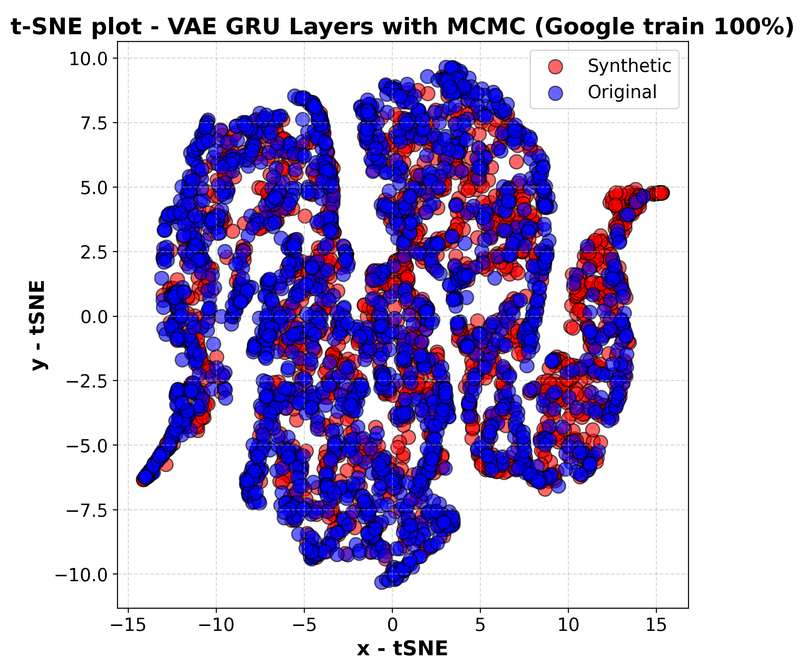
The analysis of the results shows that the use of 90% of the data for training, compared to 100% as in TimeGAN, did not significantly affect the performance of the model. As per

Table 3. Quantitative metrics.

Dataset	Discriminative Score	Predictive Score
Google Model (90% Train)	0.1985 ± 0.2159	0.0673 ± 0.0002
Google Model (100% Train)	0.1974 ± 0.2111	0.0683 ± 0.0001

and

Table 4. KS statistics.

Dataset	KS Test Statistic Value
Google Model (90% Train)	0.1319
Google Model (100% Train)	0.1048

’s metrics, including discriminative score, predictive score, and the KS test, they remained almost unchanged. The visual representation using t-SNE as per Figure 1 also shows a similar overlap between synthetic and original data, regardless of the portion of data used for training. This emphasises that the model retains its robustness even with a reduction in the training set, thus confirming the quality of the synthetic data generated.

Statistical tests provide a formal approach to assessing the quality of synthetic data, allowing a direct comparison of the statistical and temporal properties of the generated samples with those of real data. This enables the verification of whether the generative model has succeeded in preserving the essential characteristics of the time series.

Two fundamental statistical tests were considered:

• The KS test is a non-parametric statistical technique used to determine the maximum distance between the cumulative distribution functions (CDFs) of two datasets. In this case, the datasets are the real and synthetic data. The objective is to determine whether the synthetic data follow the same statistical distribution as the real one.
• The autocorrelation function is a statistical measure that assesses the degree of dependence of a time series on its past values. The test allows the comparison of temporal patterns between real and synthetic data by analysing the consistency of sequential dependencies. The aim is therefore to determine whether the synthetic data preserve the inherent temporal relationships present in the real data.

Table 5. KS test statistic values for different VAE models.

Model	KS Test
VAE—Conv Layers	0.33567
VAE—GRU Layers	0.31643
VAE—GRU Layers with MCMC	0.12772

presents the results of the KS test, which is used to ascertain the maximum distance between the cumulative distributions of the synthetic and real data for the three models under consideration. A lower value of the KS test indicates a greater similarity between the two distributions. The results for the models with convolutional and GRU layers demonstrate a notable divergence between the two distributions, suggesting a limitation in accurately capturing the underlying data distribution. In contrast, the model with MCMC sampling integration exhibits a significantly lower KS test value than the first two models, indicating a smaller discrepancy between the synthetic and real data distributions and a greater capacity to accurately represent the underlying characteristics.

Figure 2 illustrates the difference of the autocorrelation function (ACF) between real and synthetic data for the three models across a range of lag values. The model with convolutional layers has been demonstrated to be effective for low lags but shows difficulties in capturing long-term correlations, highlighting a limited ability to model the extended temporal relationships present in the real data. In contrast, the VAE model with GRU exhibits difficulties in the short term but the results are more effective in representing long-term correlations. Finally, the VAE model with GRU and MCMC sampling shows a more stable curve, exhibiting minimal variation across lag levels. This suggests that the model is more consistent in its representation of both short- and long-term temporal dependencies of the real data than the other two models, thus representing an appropriate compromise between the two models.

Visual evaluations constitute a supplementary instrument to quantitative metrics and statistical tests, offering an intuitive comprehension of the quality of synthetic data generated. By employing dimensionality reduction techniques, it is feasible to examine the distribution of synthetic and real data in a two-dimensional space, thereby facilitating the discernment of their overlap or any notable discrepancies.

In this case, t-SNE was used: it is a non-linear technique that reduces the dimensionality of datasets by emphasising local relationships between data points.

The t-SNE plots of the synthetic data generated by the different models developed in this study are shown.

In the case of the VAE model with convolutional layers, Figure 3, the image shows a good overlap between the synthetic and real data, with the former correctly following the general trend of the latter. However, there are discrepancies in the representation of internal clusters, suggesting that the model has difficulties in capturing the more sensitive details of the real data.

With the VAE model with the GRU layer, Figure 4, the overlap between synthetic and real data appears to be better defined, indicating a greater ability to represent sequential structure. In addition, the model produces data with greater breadth, allowing more information to be captured compared to the model with convolutional layers.

The VAE model with GRU layers and MCMC sampling, Figure 5, shows the most accurate overlap between synthetic and real data, which correctly follows the original trend and also ensures a more uniform and balanced distribution of the synthetic data across the space in which the real data are distributed. This approach therefore allows the model to better capture even the most specific features of the real data.

In summary, the integration of MCMC sampling appears to have significantly improved the flexibility and accuracy of the model in representing the distribution of the real data.

5.3. Robustness Analysis

A further analysis was conducted to evaluate the robustness of the final model in the presence of missing data, which is a common condition in real datasets. This evaluation was conducted by simulating the introduction of increasing proportions of missing values into the dataset, with a uniform random distribution both over time and between variables.

The objective of this test was to assess the impact of increasing missing data on the quality of the synthetic data generated, using the same evaluation metrics employed in the previous analyses. Therefore, the goal is to identify the operational limits of the model, establishing the threshold beyond which the considered architecture is no longer capable of generating data with an acceptable quality.

Figure 6 and Figure 7 show the performance of two main metrics, the KS statistic and the discriminative score, as a function of the variation in the percentage of missing values, from 0% to 60%. These are considered for the final model and the model with the GRU layers but employing traditional latent sampling. The results show a progressive deterioration in the performance of the final model as the percentage of missing values increases, highlighting the difficulty of preserving patterns and temporal relationships under conditions of incomplete data.

However, the final model shows greater robustness than approaches based solely on traditional sampling techniques. In particular, the discriminative score of the model with MCMC sampling exhibits less deterioration, remaining up to 30% missing values at levels similar to those of the model with no missing values, and then converging to the scores observed in the basic GRU model. Regarding the KS test, the increase in the value of the statistic is less pronounced in the final model with MCMC sampling than in the GRU model with traditional sampling.

In addition to the robustness of the synthetic data generated, assessing the model’s ability to handle the presence of missing data, it is also important to evaluate the capacity to augment the dimensionality of the original dataset. Data augmentation is a fundamental technique, especially when employing analysis and prediction models in scenarios with a limited availability of data for training. In this context, generative models can support the creation of significantly larger datasets than the original ones, thereby enabling more robust training of machine learning models.

In detail, the final model developed, a VAE with GRU layers and MCMC sampling, has been used to progressively generate an increasing volume of synthetic data. This strategy has been supported by the examination of the advancement in predictive performance, quantified by the predictive score, which assesses the model’s capacity to accurately predict real data when trained on synthetic data.

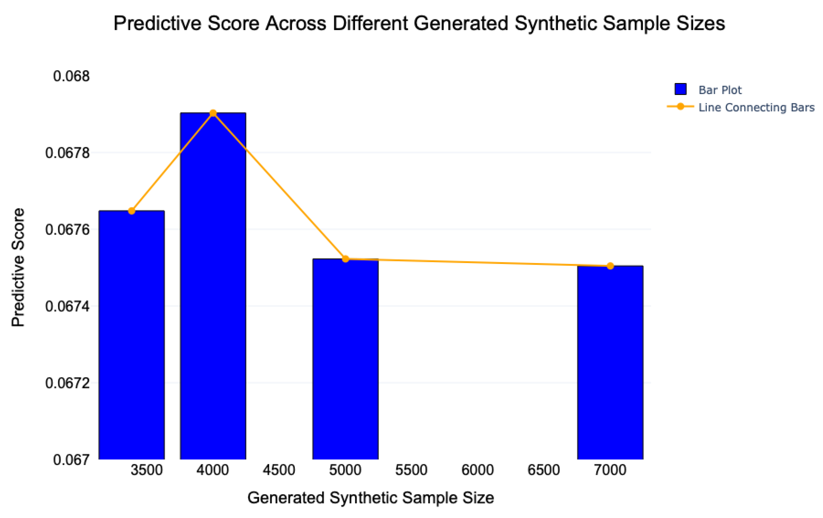
In addition to the scenarios previously analysed, in which the number of synthetic samples was equal to that of the real data, further experiments have been conducted with the generation of synthetic datasets comprising 4000, 5000, and finally, 7000 observations, which is almost equal to twice the original dimensionality.

Figure 8 illustrates the scenario mentioned above, showing the trend of the predictive score concerning the generation of synthetic data with progressively increasing dimensionality. From this, it can be observed that the predictive score remains relatively consistent in comparison to that obtained with a dimensionality equal to that of the original dataset. However, a reduction in the score is evident in the samples comprising 5000 and 7000 units. This outcome demonstrates the model’s capacity to generate a considerable number of units in comparison to the source data, thereby maintaining statistical properties across the entirety of the dataset.

This characteristic is essential for the effective implementation of data augmentation, which enables the training of more robust and accurate predictive models. The capacity of the model to maintain a balance between the generation of synthetic data and the retention of the fundamental characteristics of the original dataset represents a pivotal aspect in reinforcing the performance of machine learning models in data-poor contexts.

5.4. Model Parametrization

Table 6. Model VAE-GRU without MCMC.

Hyperparameter	Value
Sequence length	14
Feature dimension	6
Latent space dimension	8
Hidden layer sizes	[50, 100, 200]
initial_learning_rate	0.001
decay_steps	3000
decay_rate	0.9
Activation function	relu
Dropout rate	0.01
Reconstruction weight	3
Batch size	16
Max epochs	100
Verbose	30

,

Table 7. Model VAE-GRU with MCMC.

Hyperparameter	Value
Sequence length	14
Feature dimension	6
Latent space dimension	8
Hidden layer sizes	[64, 128, 256]
initial_learning_rate	0.001
decay_steps	3000
decay_rate	0.9
Activation function	relu
Dropout rate	0.01
Reconstruction weight	3
Batch size	16
Max epochs	150
Verbose	30

and

Table 8. MCMC sampling parameters.

Hyperparameter	Value
Number of samples	50
Hidden dimension (GRU)	32
Latent dimension	8

show the model parameters and the execution time of VAE-GRU without and with MCMC.

During the training, the RAM Memory was 277.21 MB, while the time was 613.25 s (10.22 min).

Training time was 1296.35 s (21.60 min); RAM Memory used was 397.73 MB.

To improve the selection of hyperparameters and the robustness of the results, two main strategies were implemented, an intensive tuning of the model’s hyperparameters and the adoption of cross-validation. Through the use of a hyperparameter optimisation framework, it was possible to explore a wider range of model configurations. The research involved the exploration of the following values for each hyperparameter:

• Size of latent space: values explored between 4, 8, 16 and 32.
• Size of hidden levels: for each of the three hidden levels, values between 32 and 256 were tested in steps of 32.
• Learning rate: values of 0.01, 0.001, 0.0005, and 0.0001 were tested.
• Dropout rate: dropout rates of 0.01, 0.1, 0.2, and 0.3 were evaluated to improve generalisation ability.
• Reconstruction weight: values explored include 1, 3, 5, and 10.
• Batch size: batch sizes 8, 16, 32, and 64 were tested.

The approach allowed the various configurations to be evaluated with up to 150 epochs and a reduction factor of 3. The metric used to optimise the model was the validation loss. At the end of the process, val_loss was 71.47171020507812. The best hyperparameters are characterised by

Table 9. Hyperparameter tuning results.

Hyperparameter	Best Value So Far
latent_dim	32
hidden_size_0	160
hidden_size_1	160
hidden_size_2	128
learning_rate	0.001
dropout_rate	0.03
reconstruction_wt	1
tuner/epochs	150
tuner/initial_epoch	50
tuner/bracket	2
tuner/round	2
tuner/trial_id	196

:

To further improve the robustness and generalisability of the results, cross-validation with five folds using the KFold library was adopted. This approach allowed the dataset to be divided into five subgroups, alternating the roles of training and validation. Each model was trained for a maximum of 150 epochs in each fold. Quantitative metrics and KS statistics are shown in

Table 10. Quantitative metrics.

Dataset	Discriminative Score	Predictive Score
Google Model (100% Train)
Optimal Hyperparameter	0.2014 ± 0.2199	0.0662 ± 0.0004
Google Model (100% Train)	0.1975 ± 0.2112	0.0684 ± 0.0002

and

Table 11. KS statistics.

Dataset	KS Test Statistic Value
Google Model (100% Train)
Optimal Hyperparameter	0.1655
Google Model (100% Train)	0.1049

.

Figure 9 presents a t-SNE plot illustrating the synthetic data generated by the VAE-GRU-MCMC model for Google stock prices using the best-selected hyperparameters. The purpose of this visualisation is to assess the degree to which the synthetic data distribution aligns with the real data distribution, serving as a qualitative validation of the model’s generative capabilities.

The plot demonstrates a strong overlap between the real and synthetic data, indicating that the model successfully captures the statistical and temporal structure of Google’s stock price movements. Compared to previous t-SNE plots in the study, this representation suggests that the refined hyperparameter tuning has further improved the quality of the generated sequences, leading to a more faithful reproduction of the original dataset. The synthetic points appear well integrated within the real data clusters, reinforcing the idea that the model does not merely replicate general trends but also retains the finer details and variations inherent in the stock price dynamics.

By comparing Figure 9 with earlier versions of the model’s outputs, one can observe a clear enhancement in performance due to hyperparameter optimisation. The improved latent space representation, facilitated by the combination of GRU layers and MCMC sampling, enables a more effective learning process, ensuring that the generated data maintain structural coherence with the real dataset. The lack of significant outliers or unnatural clustering patterns suggests that the model effectively mitigates issues such as mode collapse, which is a common challenge in generative models.

The obtained results demonstrate, as per Figure 1 and Figure 9 that the optimised model, with intensive tuning and cross-validation, attains a performance that is highly analogous to that of the previous shared model, despite the increased methodological rigour. Quantitative metrics and the KS test exhibits minimal disparities, thereby confirming comparable quality in data generation and prediction, and a statistically similar distribution. The t-SNE representations further highlight a similar overlap between synthetic and original data. This finding suggests that the initial model was effectively set up.

6. Generalisation to Different Datasets

The incorporation of MCMC sampling into the VAE-GRU network has been shown to significantly improve the performance and quality of the generated synthetic data. However, this enhancement comes at the expense of increased computational cost. Specifically, the training time increased from approximately 10.22 min (613 s) to 21.61 min (1296 s), accompanied by a rise in RAM usage from 277 MB to 398 MB. This trade-off highlights that the improved accuracy and robustness achieved through MCMC sampling necessitate a more resource-intensive training process. Nonetheless, these additional computational requirements yield substantial improvements in model performance, particularly in terms of the realism and precision of the generated synthetic data. In applications where the fidelity of synthetic outputs or the robustness of the model is paramount—such as in research or industrial scenarios—this increase in computational demand is justified.

To comprehensively evaluate the model’s generalisation capabilities and adaptability across varying levels of volatility, demand cycles, and sector-specific dynamics, additional analyses were conducted beyond the initial focus on Google’s stock. Specifically, the model was assessed using data from Tesla and Nestlé stocks, representing distinct industries and geographical contexts. A common time window was selected to ensure consistency and comparability across these evaluations.

The findings derived from the analysis of three distinct evaluation approaches, quantitative metrics (as per

Table 12. Discriminative and predictive scores for different datasets.

Dataset	Discriminative Score	Predictive Score
Google	$0.1985\pm 0.2159$	$0.0673\pm 0.00026$
Tesla	$0.1963\pm 0.2128$	$0.0913\pm 0.0002$
Nestlè	$0.2023\pm 0.22819$	$0.0611\pm 0.0002$

), statistical tests (as per

Table 13. Kolmogorov–Smirnov test (KS test) statistic values for different datasets.

Dataset	KS Test Statistic Value
Google	$0.1318$
Tesla	$0.1256$
Nestlè	$0.1130$

), and t-SNE plot analysis (as per Figure 5, Figure 10, Figure 11 and Figure 12), demonstrate that the final VAE-GRU model with MCMC sampling, previously assessed using Google stock data, achieves superior performance when applied to other categories of stock data. The discriminative and predictive scores highlight the model’s ability to generate synthetic data that closely mirror the corresponding original data.

In Figure 5, which depicts the t-SNE representation for Google stock data, there is a strong overlap between the real and synthetic points. This suggests that the model successfully learns and replicates the patterns present in Google’s historical prices. The synthetic distribution follows the real one closely, indicating that key statistical and temporal characteristics are well preserved. The presence of well-defined clusters further confirms that the model is capturing the local structures of the data rather than producing overly smoothed or distorted distributions.

Figure 10, which presents the t-SNE plot for Tesla stock data, shows a similar trend, though with slightly more variance in the synthetic data. Tesla’s stock is known for its high volatility and rapid fluctuations, making it a more challenging dataset to model accurately. While the generated data largely align with the real distribution, some discrepancies appear, particularly in the finer details of certain clusters. This suggests that while the model can reproduce general trends and patterns in Tesla’s price movements, it may struggle to fully capture the extreme fluctuations characteristic of this stock.

In contrast, Figure 11, which illustrates the t-SNE plot for Nestlé stock data, exhibits an almost perfect alignment between the synthetic and real distributions. Since Nestlé’s stock is generally less volatile than Tesla’s, the model is able to generate synthetic data that closely mirror the real time series without significant deviations. The clusters in this plot are tightly packed, and the overall dispersion of synthetic points closely matches that of the real data, indicating that the model has successfully learned the underlying structure of Nestlé’s price movements with a high degree of accuracy.

Figure 12 provides a different perspective by analyzing the ACF differences between real and synthetic data across different lag values for the three stock datasets. The ACF measures how past values influence future values in a time series, making it a critical test for evaluating whether a generative model has successfully captured the temporal dependencies of the original data. The results show that the synthetic Google stock data exhibit the smallest ACF differences, meaning that its temporal structure is closely aligned with the real dataset. The Tesla stock data, on the other hand, presents slightly higher ACF differences, which confirms the observation from the t-SNE analysis that extreme market movements are harder for the model to replicate. The Nestlé dataset falls in between, demonstrating that the model performs well with moderate volatility but may struggle with extreme fluctuations.

To calculate the predictive score, a recurrent neural network model based on the GRU was developed. The architecture of the model is defined as follows:

• Masking: the first layer applies a mask to the input data to handle variable length sequences and ignore padding values.
• GRU cell: the core of the model is a GRU cell with tanh activation and hidden layer size equal to half the size of the original feature space (hidden_dim = dim/2).
• Dense layer: the output of the GRU is passed through a dense layer with sigmoid activation to generate the final prediction.

Training takes place following these steps:

• The generated synthetic data are split into mini-batches of size 128.
• The model is trained for 5000 iterations using the Adam optimiser, minimising the absolute difference loss function between predicted and actual values.
• After training, the model is tested using real data to measure its predictive ability on the original sequences.

The predictive score is calculated as the mean absolute error (MAE) between model predictions and actual values. This value aims to reflect how well the synthetic data can maintain temporal and structural consistency with the original time series.

Specifically, t-SNE visual inspection reveals the model’s capacity to effectively capture the structure of the original data and preserve their nuanced characteristics, regardless of the specific stock context under consideration.

The tuning process of the hyperparameters (see

Table 14. VAE hyperparameters.

Parameter	Value
Sequence length	14
Feature dimension	6
Latent space dimension	8
Hidden layer sizes	[64, 128, 256]
initial_learning_rate	0.001
decay_steps	3000
decay_rate	0.9
Activation function	relu
Dropout rate	0.01
Reconstruction weight	3
Batch size	16
Max epochs	150
Verbose	30

and

Table 15. MCMC sampling parameters.

Parameter	Value
Number of samples	50
Hidden dimension (GRU cell for transition dynamics)	32
Latent dimension	8

) involved a continuous increase in the complexity of the VAE architecture to capture the more specific characteristics of the original data.

The training process, performed without a GPU, required 1296.3557 s (approximately 21.61 min) and consumed a peak of 397.73 MB of RAM.

Energy and Air Quality Datasets

To further evaluate the capabilities of the proposed model, it was decided to extend the experimental analysis by including two new datasets from the UCI Machine Learning Repository:

• Energy: a dataset predicting the energy consumption of household appliances, consisting of 19,735 samples with 28 continuous variables [23].
• Air: a dataset containing air quality measurements, with 9357 samples and 15 data characteristics averaged hourly [24].

This extension of the analysis allows the model to be tested on more diverse data than previous financial datasets (Google, Tesla, Nestlé). The objective is to assess its generalisation capacity considering key metrics such as the KS test and the quantitative scores. The results obtained on these new datasets are presented in

Table 16. Quantitative metrics.

Metric	Value	Unit	Description
Accuracy	95.4%	Percentage	Correct classifications
Precision	92.1%	Percentage	Positive predictive value
Recall	90.3%	Percentage	Sensitivity
F1-score	91.2%	Percentage	Harmonic mean of precision and recall
AUC-ROC	0.96	-	Area under the ROC curve

and

Table 17. KS statistics.

Dataset	KS Test Statistic Value
Google	0.1319793205317578
Energy	0.23539117850329408
Air	0.2550334166844218

.

The model shows similar performances on the two new datasets. Analysing the quantitative metrics, the discriminative score is almost unchanged, while the predictive score shows significantly better performance on the air quality data. Overall, the results are good and in line with those obtained on the stock datasets. The t-SNE analysis, as per Figure 13 and Figure 14, confirms a good overlap between synthetic and real data for both new datasets, although a slight higher bias emerges compared to the stock datasets. This is also supported by the KS test, which shows a higher value, indicating a more pronounced difference between the synthetic and real data distributions.

Specifically, in Figure 13, which corresponds to the energy consumption dataset, there is a noticeable degree of overlap between the real and synthetic data distributions. This indicates that the model successfully captures key patterns in the dataset, generating synthetic sequences that align well with the real data. However, compared to the t-SNE plots of the stock price datasets, the separation between clusters appears slightly more pronounced, suggesting that while the model maintains the overall structure of the data, it may introduce minor deviations in certain localised regions. This could be attributed to the complex, multi-variable nature of energy consumption data, where external factors such as weather, household behaviour, and regional characteristics contribute to variations that may be harder to replicate perfectly.

Similarly, Figure 14, which represents the Air Quality dataset, shows a reasonable alignment between real and synthetic data, though with slightly greater dispersion compared to the Energy dataset. This suggests that while the synthetic data follow the general structure of the original dataset, some finer details in the local patterns are not perfectly captured. The Air Quality dataset, which consists of various environmental indicators such as pollutant levels and meteorological conditions, exhibits a high degree of variability influenced by external and often stochastic factors. The wider spread in the t-SNE representation indicates that the model encounters more difficulty in fully capturing these complex interactions compared to financial or energy-related data.

Finally, Figure 15 indicates a general decline in ACF differences as the lag increases, suggesting that short-term dependencies are more challenging to replicate accurately than long-term correlations. The Google dataset exhibits the smallest ACF differences, indicating that the synthetic data closely follow the real data’s temporal structure. In contrast, the Air Quality and Energy datasets display higher ACF differences, particularly at lower lags, suggesting that the synthetic model struggles to replicate short-term dependencies in these datasets. Despite these differences, the ACF trends stabilize at higher lags, indicating that the model effectively captures long-term dependencies across datasets. These findings reinforce the robustness of our method while also highlighting potential areas for improvement, particularly in refining short-term dependency modelling for certain dataset types.

7. Discussion

The results presented in the experiments demonstrate that the proposed VAE-GRU-MCMC model is highly effective in generating synthetic financial time series that closely resemble real stock price movements. The quantitative evaluations, including the discriminative and predictive scores, confirm that the model successfully preserves statistical and temporal properties, making it a competitive alternative to existing generative approaches such as TimeGAN. However, beyond these numerical results, a deeper analysis is necessary to interpret the implications of these findings, compare them with existing models, and understand the limitations and areas for future improvements.

One of the most significant contributions of this study is the hybridisation of VAE with MCMC sampling, which introduces a more structured latent space exploration. The comparison with baseline models, such as the convolutional VAE and GRU-based VAE, highlights the importance of capturing long-term dependencies in financial time series. While convolutional layers are effective in learning local patterns, they struggle with sequential dependencies, leading to less accurate synthetic data. The transition to GRU layers allowed the model to learn temporal structures more effectively, as reflected in improved discriminative and predictive scores. Furthermore, the integration of MCMC sampling refined the latent space representation, reducing divergence between real and synthetic distributions. This approach provided more stable and robust synthetic data, as confirmed by the lower KS test values.

Compared to TimeGAN, which has been considered a state-of-the-art generative model for sequential data, the VAE-GRU-MCMC model demonstrates competitive performance while maintaining a simpler and more interpretable architecture. TimeGAN integrates an adversarial training mechanism, which, while effective, can suffer from issues such as mode collapse and training instability. In contrast, the proposed model avoids these problems by leveraging variational inference and structured sampling techniques. The results indicate that although TimeGAN marginally outperforms the VAE-GRU-MCMC model in some metrics, the latter offers advantages in computational efficiency and ease of implementation, making it a viable alternative for synthetic financial data generation.

The ability to generate high-quality synthetic stock price data has several practical applications. In finance, synthetic data can be used to augment training datasets for predictive modelling, reducing dependency on historical data that may be subject to confidentiality constraints. This is particularly useful for stress testing trading algorithms, where diverse market conditions must be simulated. The model’s demonstrated robustness to missing data also makes it suitable for financial environments where datasets are often incomplete due to reporting delays or data corruption. Additionally, the ability to generalise to non-financial datasets, such as energy consumption and air quality data, suggests that the methodology can be extended to other domains where sequential data are prevalent.

Despite its strong performance, the proposed model has certain limitations. The analysis of synthetic stock price data for Google, Tesla, and Nestlé revealed that while the model performs well for stable and moderately volatile stocks, it struggles slightly with highly volatile assets such as Tesla. This suggests that the model may not fully capture extreme fluctuations in stock prices, which could be addressed by incorporating additional mechanisms, such as attention layers, to better model volatility.

Another limitation concerns computational efficiency. While the VAE-GRU-MCMC model is more stable than GAN-based methods, the integration of MCMC sampling increases training time compared to traditional VAE approaches. Future work could explore more efficient sampling techniques or hybrid methods that balance stability and computational cost.

Moreover, the current study primarily focuses on one-dimensional financial time series. Expanding the approach to handle multi-modal data, such as the joint modelling of stock prices, trading volume, and macroeconomic indicators, could provide a more comprehensive framework for synthetic financial data generation. Additionally, the inclusion of reinforcement learning techniques for adaptive latent space exploration could further enhance the model’s ability to generate diverse and high-quality synthetic sequences.

8. Conclusions and Future Work

This study presents an innovative methodology for generating robust synthetic sequential data, addressing key challenges in financial time series modelling. By integrating GRU-enhanced VAE with MCMC sampling, the proposed model achieves superior fidelity in representing the intricate dynamics of financial data. Experimental results highlight its resilience across diverse datasets, including Google, Tesla, and Nestlé stock prices, and its robustness under varying proportions of missing data. Quantitative metrics and statistical tests confirm the model’s ability to produce synthetic data that closely align with real-world distributions, while t-SNE visualisations illustrate its capacity to preserve nuanced temporal characteristics.

Furthermore, experiments underscore the model’s scalability in data augmentation, demonstrating consistent predictive performance even when generating datasets nearly double the size of the original. These capabilities make the model an attractive alternative to GAN-based approaches, avoiding issues like mode collapse while offering computational efficiency and ease of implementation. Future work will focus on extending the model’s applicability to multi-modal and highly volatile datasets, as well as incorporating reinforcement learning techniques to further refine latent space representations.