Joint Offloading and Energy Harvesting Design in Multiple Time Blocks for FDMA Based Wireless Powered MEC

Abstract

The combination of mobile edge computing (MEC) and wireless power transfer (WPT) is recognized as a promising technology to solve the problem of limited battery capacities and insufficient computation capabilities of mobile devices. This technology can transfer energy to users by radio frequency (RF) in wireless powered mobile edge computing. The user converts the harvested energy, stores it in the battery, and utilizes the harvested energy to execute corresponding local computing and offloading tasks. This paper adopts the Frequency Division Multiple Access (FDMA) technique to achieve task offloading from multiple mobile devices to the MEC server simultaneously. Our objective is to study multiuser dynamic joint optimization of computation and wireless resource allocation under multiple time blocks to solve the problem of maximizing residual energy. To this end, we formalize it as a nonconvex problem that jointly optimizes the number of offloaded bits, energy harvesting time, and transmission bandwidth. We adopt convex optimization technology, combine with Karush–Kuhn–Tucker (KKT) conditions, and finally transform the problem into a univariate constrained convex optimization problem. Furthermore, to solve the problem, we propose a combined method of Bisection method and sequential unconstrained minimization based on Reformulation-Linearization Technique (RLT). Numerical results demonstrate that the performance of our joint optimization method outperforms other benchmark schemes for the residual energy maximization problem. Besides, the algorithm can maximize the residual energy, reduce the computation complexity, and improve computation efficiency.

1. Introduction

With the rapid advancement of 5G network and Internet of Things (IoT), countless emerging mobile application scenarios have appeared in our lives, such as artificial intelligence, internet of vehicles, augmented reality, and virtual reality. This has led to the explosive growth of IoT devices such as smartphones, intelligent wireless sensors and wearable devices [1], and the amount of data processed by IoT devices has increased dramatically. All of these have put forward higher requirements for the real-time communication and computation capabilities of mobile devices. Some researchers have combined cloud computing with mobile computing to solve the problem of limited mobile device resources. Mobile cloud computing reduces the task burden of devices by migrating some or all of the computation tasks from resource-limited mobile devices to remote clouds [2,3]. However, the disadvantages of this architecture are high overhead and long backhaul delay [4], and it is limited by network bandwidth. To solve this problem, a computing model called mobile edge computing (MEC) has received widespread attention from both industry and academia. The MEC server provides computation and storage resources for mobile devices at the edge of the network, and computation tasks can be offloaded to the edge of the network for execution, which can significantly reduce latency and reduce battery energy consumption [5].

Although MEC provides powerful computation resources for mobile devices, it still faces the challenge of limited battery energy supply. Obviously, frequent battery replacement and charging of wireless devices have brought huge costs. The emergence of wireless power transfer (WPT) technology has effectively solved the problem of insufficient energy supply of equipment. This technology broadcasts energy through radio frequency (RF) signals provided by energy transmitters to provide sustainable and permanent energy supply for mobile devices [6]. Recently, Wireless Powered Communication Network (WPCN) and Simultaneous Wireless Information and Power Transfer (SWIPT) have been proposed as important paradigms for providing real sustainability for mobile communications [7,8].

The benefits of combining WPT and MEC have been fully demonstrated in recent years. This new technology is called wireless powered MEC (WP-MEC) [9]. This paper studies the residual energy maximization problem in an environment of MEC system integrating MEC server, Access Point (AP) and multiuser. AP can deliver energy to users through radio frequency (RF). The user converts the harvested energy, stores it in the battery, and uses the harvested energy to execute corresponding computation-intensive tasks. We achieve data and energy transmission in the same frequency band through Time Division Duplex (TDD) protocol. In addition, mobile devices transmit data in FDMA manner. In this paper, we focus on jointly optimizing the wireless and computation resources for the partial computation offloading system. The main contributions of this paper are detailed as follows:

(1)

To effectively reduce the energy consumption of mobile devices, we study the multi-user dynamic joint optimization under multiple time blocks in the residual energy maximization problem. We jointly optimize the number of offloaded bits, energy harvesting time, and transmission bandwidth. To the best of our knowledge, in multiuser systems, most of the literature only studies the problem of active multiple users offloading and wireless energy transmission during one time block, and there are few works on dynamic joint optimization problems under multiple time blocks.

(2)

To solve the residual energy maximization problem of joint optimization, we propose a combined method of Bisection method and sequential unconstrained minimization based on reformulation linearization technique (RLT). We firstly derive the dual problem of the primary problem in a semi-closed form. Next, we seek for the relationship among variables by combining with the Lagrange method and KKT conditions and finally transform the problem into a univariate constrained convex optimization problem. The proposed method converts the primary problem from a nonconvex problem to a convex problem, reduces optimization variables from 3*K*N to K*N, obtains a lower computation complexity, and improves computation efficiency.

(3)

The simulation results verify the theoretical performance analysis of the proposed scheme. The results show that our scheme not only outperforms other baseline schemes but also demonstrates that our algorithm significantly improves the performance, reduces computation complexity, obtains a better solution, and can get the optimal solution.

The reminder of this paper is organized as follows. The second part discusses related work. The third part introduces the system model and problem formalization. The fourth part proposes an effective algorithm to solve the problem. The fifth part provides simulation results. The sixth part gives the conclusion.

2. Related Work

Mobile Cloud Computing (MCC) [10] can solve the problem of limited resources when mobile devices execute tasks. The studies include architecture (such as MAUI [11]) and offloading strategies (ThinkAir [12]). However, the disadvantages of this earlier scheme are high overhead and long backhaul delay. Therefore, mobile edge computing (MEC) technology has been widely studied as a network architecture that can overcome the above problems. However, the practical implementation of MEC technology still faces many challenges.

The problem of resource allocation [13,14] has always been the research focus of MEC, and one of the most critical technologies is computation offloading strategy. The mobile devices design task offloading models according to the partitionability of computation tasks, including binary offloading and partial offloading [15]. Furthermore, reference [16] proposed a wireless-powered MEC system in the unmanned aerial vehicle (UAV) scenario, studied the computation rate maximization problem under binary offloading and partial offloading modes respectively, and solved the proposed nonconvex problem by designing two-stage and three-stage algorithms. In [17], the researchers developed a reverse auction framework. They designed an offloading method based on position auction. In [18], they designed a distributed method based on game theory to manage the computation offloading tasks of wireless devices.

Only adopting the computation offloading strategy still faces the problem of insufficient computing resources and high overhead. To solve this challenge, the studies on joint optimization of energy-saving control strategies for computation and communication resources are essential. In [19], the author designed single and multiple cloud server schemes to minimize energy consumption and latency time by jointly optimizing the computing rate, transmission power and offloading rate of smart mobile devices. Literature [20] proposed a scalable approximate dynamic programming algorithm to reduce average energy consumption. In addition, ref. [21] proposed three cases including Time Division Multiple Access (TDMA) scenario, Frequency Division Multiple Access (FDMA) amplify-and-forward (AF) mode, and scenario in decode-and-forward (DF) mode to minimize the total energy consumption in the system. In [22], orthogonal frequency division multiple access (OFDMA) and time division multiple access (TDMA) systems with infinite or limited cloud computing capabilities formulate the optimal resource allocation problem as a convex optimization problem to solve the minimization problem of the weighted sum mobile consumed energy under computation delay constraints. Furthermore, ref. [23] proposed joint resource allocation and user selection algorithm in MEC to maximize the energy efficiency of the mobile device. In addition, ref. [24] proposed an energy-saving routing scheme that combines the mobile sink and the static sink to decrease the corresponding transmission latency and significantly increase network lifetime. In [25], they proposed an algorithm of jointly allocating bandwidth and computational resources to mobile devices to minimize the energy consumption.

As the basic strategy of the MEC system, in recent years, computation offloading methods for Time Division Multiple Access (TDMA) [26], Orthogonal Frequency Division Multiple Access (OFDMA) [27], and Code Division Multiple Access (CDMA) [28] are widely studied. In [29], work is done to minimize the weighted sum energy at the edge server and the users by FDMA technique with the constraints of the limits of computation, communication and caching capacities, as well as the computation latency. In [30], the energy minimization problem of the offloading system based on the OFDMA scheme in 5G heterogeneous networks is studied. This scheme jointly optimizes wireless and offloading resource allocation. In [31], based on the TDMA technique, the total energy consumption of the AP is minimized by jointly optimizing the CPU frequency, the energy transmit beamforming from the AP transmitter, and the number of offloading bits at the users. An offloading algorithm is proposed in [32] to minimize latency by jointly optimizing the computation and radio resources in a multiuser system.

The research mentioned above basically focuses on saving energy. However, it still faces the problem of insufficient battery energy supply. Wireless power supply technology can avoid frequent battery replacement to improve the sustainability of mobile devices effectively. In [33,34,35,36,37], WPT technology can provide mobile users with continuous wireless energy supply through energy transmitters, and the user can execute task computing and offloading by utilizing the acquired energy. Energy harvesting and resource allocation can significantly improve the performance of the overall system. In [38], they jointly optimizing remote task execution, the energy beamforming at the AP, the task offloading and local computing to solve the problem of the system energy consumption minimization. In [39], they proposed a low-complexity online algorithm based on Lyapunov optimization to minimize the execution cost. In [40], the energy transmission variance, transmission power, and transmission time were jointly optimized to maximize the energy efficiency of the multiantenna WPCN system. In [41], two schemes were proposed for WPCN, which integrates the “harvest-then-transmit” (HTT) mode and the backscatter mode. The research improved the throughput of the total system by applying the user’s working mode.

The practical implementation of the WPT-MEC system still faces many challenges, such as channel fluctuations, dynamic task arrivals, caching mechanisms, unmanned aerial vehicle (UAV), and device status changes. To solve the challenges, in the recent literature [42], the energy consumption of dynamic task arrivals over time and channel fluctuations was studied. They developed heuristic online designs for the joint WPT energy and computation resources to minimize energy. In [38], they considered the dynamic changes of channel state information (CSI) and task state information (TSI), the paper significantly improved the energy efficiency of the system by integrating with the sequential optimization method. In [43], the anti-interference UAV powered cooperative MEC scheme was proposed to minimize the transmit energy of the UAV. Considering that there are few studies on the dynamic joint optimization of the device state, this thus motivates our study in this work.

Different from the previous work, this paper mainly studies the maximum residual energy of the multiuser dynamic joint optimization of the number of offloaded bits, the energy harvesting time, and the transmission bandwidth under multiple time blocks. As far as we know, in the work aimed at maximizing the residual energy of mobile devices, most of the work focuses on the joint optimization of active single user under single time block. There are few studies on this challenge of our work. In our research, all device states change randomly (active or silent). In real scenario, mobile devices cannot always be in working state. Therefore, our work not only achieves joint optimization of resource allocation and improves algorithm efficiency but also increases the possibility of practical implementation of the WPT-MEC system.

3. System Model and Problem Formulation

3.1. System Model

As shown in Figure 1, the residual energy maximization problem is studied in an environment of MEC system. The system includes an Access Point (AP) integrated with the MEC server and K mobile devices. The mobile devices are denoted by $M{D}_i$, $i\in {\rm K}=\left\{1,2\dots \dots K\right\}$. The AP adopts RF signal-based radio to charge K mobile devices, then receives offloaded tasks from users and transmits them to MEC for computing. AP provides energy to mobile devices by transferring RF power. The mobile devices receive and convert RF power into energy in their batteries and utilize the stored energy to execute task computation. Assume that the downlink energy transmission from AP to users and the uplink computation offloading from users to AP are implemented in the same frequency band, a block system based on FDMA is applied. Besides, the channel state remains constant in one time block and varies between different time blocks. t denotes the time block index, and $t\in \mathcal{T}=\left\{0,1,2,\dots ,N\right\}$. T denotes one time block length. Each wireless device includes two states: active or invalid. It is assumed that the device state of each wireless device $M{D}_i$ at each time block $t\in \mathcal{T}$ is denoted by $s_i\left(t\right)\in \left\{0,1\right\}$, (0 means invalid, 1 means active). Define the device status of all mobile devices $M{D}_i$ during the t-th time block as $S\left(t\right)=\left\{s_1\left(t\right),s_2\left(t\right),\dots ,s_K\left(t\right)\right\}$. Furthermore, we assume that the channel state information (CSI) from/to K mobile devices can be perfectly known by the AP [44]. Denote the uplink channel power gain vector in the t-th time block as $H\left(t\right)=\left\{h_{1,u}\left(t\right),h_{2,u}\left(t\right),\dots ,h_{K,u}\left(t\right)\right\}$. Similarly, the downlink channel power gain vector is denoted by $G\left(t\right)=\left\{g_{1,d}\left(t\right),g_{2,d}\left(t\right),\dots ,g_{K,d}\left(t\right)\right\}$. Where $h_{i,u}^{max}<\infty$, $g_{i,d}^{max}<\infty$, $i\in {\rm K}$.

Figure 1. System architecture.

Figure 2 shows the harvesting and offloading model. The mobile devices offload data in the FDMA manner. Assume that the time block length is T. In the t-th time block, the first $T_{i,h}\left(t\right)$ denotes the time for each mobile device to harvest energy from the AP, and the second $T_{i,o}\left(t\right)$ denotes the time to offload tasks from mobile devices to the AP, the execution of the offloading tasks and the download of the computing results are accomplished within the remaining time of the time block. Assume that downlink RF signals transfer and local computing are executed simultaneously.

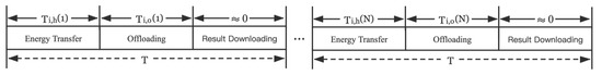
Figure 2. The time allocation.

3.2. Computing Model

In each time block t, the computation task for each user $i\in {\rm K}$ is partitioned into two parts. Assume that the total computation task is $Z_i\left(t\right)\ge 0$, local and offloading computing are represented by $l_i\left(t\right)\ge 0$ and $q_i\left(t\right)\ge 0$ (bit).

3.2.1. Local Computing Model at Active Users

First, consider the local computing for executing $l_i\left(t\right)$ input bits. Assume that it can be known through off-line measurement that it takes $C_i$ CPU cycles to process one bit at $M{D}_i$. The wireless device can adjust the CPU clock rate by the Dynamic Voltage and Frequency Scaling (DVFS) technology. In the t-th time block, let $f_{i,m}\left(t\right)$ denote the adjustable CPU cycle frequency, $m\in \left\{1,2,\dots ,C_i{l}_i\left(t\right)\right\}$. This frequency cannot exceed the limit of the maximum CPU frequency; it is denoted by $f_i^{max}$, which depends on the chip architecture. This constraint is as follows:

$$0<f_{i,m}\left(t\right)\le f_i^{max},\forall i\in K,\forall t\in \mathcal{T}$$

(1)

As local computing should be accomplished within the block, we have the computation latency constraints as follows:

$${{\displaystyle \sum }}_{m=1}^{C_{\mathrm{i}}{l}_i\left(t\right)}\frac{1}{f_{i,m}\left(t\right)}\le T,\forall i\in K,\forall t\in \mathcal{T}$$

(2)

Thus, the consumed energy for the above discussions at a mobile device can be expressed as:

$$E_{i,\mathrm{loc}}={{\displaystyle \sum }}_{m=1}^{C_{\mathrm{i}}{l}_i\left(t\right)}{\zeta }_i{f}_{i,m}^2\left(t\right),\forall i\in K,\forall t\in \mathcal{T}$$

(3)

where ${\zeta }_i>0$ represents the effective capacitance coefficient and the microscale relies on the chip architecture at user i [45], we ${\zeta }_i={10}^{-28}$ according to the actual measurement. To minimize the consumed energy as much as possible while satisfying the delay constraints, it is optimal for each mobile device to set the CPU frequency to be identical. By satisfying strict equality of the constraints in (2), we obtain the following equation:

$$f_{i,1}\left(t\right)=\cdots =f_{i,C_{\mathrm{i}}{l}_i\left(t\right)}\left(t\right)=C_{\mathrm{i}}{l}_i\left(t\right)/T,\forall i\in K,\forall t\in \mathcal{T}$$

(4)

The maximum CPU cycle frequency is $f_i^{max}$ for each user, so the number of computation bits by local computing is constrained by:

$$0\le l_i\left(t\right)\le \frac{T{f}_i^{max}}{C_{\mathrm{i}}},\forall i\in K,\forall t\in \mathcal{T}$$

(5)

As the total computation task is composed of local and offloading computing, we have $Z_i\left(t\right)=l_i\left(t\right)+q_i\left(t\right)$, the following constraints can be obtained:

$$Z_{\mathrm{i}}\left(t\right)-\frac{T{f}_i^{max}}{C_{\mathrm{i}}}\le q_i\left(t\right)\le Z_{\mathrm{i}}\left(t\right),\forall i\in K,\forall t\in \mathcal{T}$$

(6)

Accordingly, the energy consumption of $E_{i,\mathrm{loc}}\left(t\right)$ can be expressed as follows:

$$E_{i,loc}\left(t\right)=\frac{{\zeta }_i{C}_i^3{\left(Z_{\mathrm{i}}\left(t\right)-q_i\left(t\right)\right)}^3}{T^2},\forall i\in K,\forall t\in \mathcal{T}$$

(7)

3.2.2. Offloading Model from Active Users to the AP

Consider the offloading computing for executing $q_i\left(t\right)$ offloaded bits in any time slot. The mobile device offloads its task to the AP by the FDMA offloading strategy. Then, the offloading computing will be performed by the edge server integrated with the AP. The data transmission rate for user i in the t-th time block is expressed as:

$$v_{i,o}(t)={\beta }_{i,o}(t){\log }_2(1+\frac{p_{i,o}\left(t\right)h_{i,u}\left(t\right)}{{\sigma }^2}),\forall i\in K,\forall t\in \mathcal{T}$$

(8)

where $p_{i,o}\left(t\right)$ is the uplink data transmission power from the user i to the MEC. ${\sigma }^2$ denotes the noise power at the AP receiver, ${\beta }_{i,o}\left(t\right)$ denotes the bandwidth allocation vector for the mobile device i in each time block t. As the shared bandwidth of K users cannot exceed the total bandwidth, the following constraints can be obtained:

$${{\displaystyle \sum }}_{i=1}^K{\beta }_{i,o}\left(t\right)\le B,\forall i\in K,\forall t\in \mathcal{T}$$

(9)

where B denotes the total bandwidth of the channel. Then, the offloading time from the $M{D}_i$ to the AP can be expressed as:

$$T_{i,o}\left(t\right)=\frac{q_i\left(t\right)}{v_{i,o}\left(t\right)},\forall i\in K,\forall t\in \mathcal{T}$$

(10)

As harvesting and offloading time cannot exceed the time slot length T, there are the following constraints:

$$T_{i,h}\left(t\right)+\frac{q_i\left(t\right)}{v_{i,o}\left(t\right)}\le T,\forall i\in K,\forall t\in \mathcal{T}$$

(11)

Computation offloading incurs energy consumption. In addition to the transmission power $p_{i,o}\left(t\right)$ the constant circuit power $p_{c,i}>0$ is consumed. It is obtained that the energy consumption (J) of task offloading for user i can be expressed as:

$$E_{i,off}\left(t\right)=p_{i,o}\left(t\right)T_{i,o}\left(t\right)+p_{c,i}{T}_{i,o}(t),\forall i\in K,\forall t\in \mathcal{T}$$

(12)

Consider the limit of the computation capability of the MEC server. $Q_{\max }$ denotes the maximum number of computation cycles executed at the edge server during t-th time block. Then, we have:

$${{\displaystyle \sum }}_{i=1}^K{q}_i\left(t\right)C_{\mathrm{i}}\le Q_{\max },\forall i\in K,\forall t\in \mathcal{T}$$

(13)

This constraint can guarantee that the MEC computation latency is negligible.

3.3. Energy Harvesting Model

In each time block t, the AP can transfer the RF signals at an energy transmit power $P_d\left(t\right)$ to charge the mobile device [6]. The mobile device harvests the energy and stores it in the battery after conversion. Therefore, the energy harvested by the i-th mobile device is:

$$E_{i,h}\left(t\right)={\eta }_i{T}_{i,h}\left(t\right)P_d\left(t\right)g_{i,d}\left(t\right),\forall i\in K,\forall t\in \mathcal{T}$$

(14)

where $0<{\eta }_i<1$ represents the energy conversion efficiency.

We combine the offloading computing energy and the local computing energy, the overall energy consumption at user i in the t-th time block is given by:

$$E_{i,c}\left(t\right)=E_{i,loc}\left(t\right)+E_{i,off}\left(t\right),\forall i\in K,\forall t\in \mathcal{T}$$

(15)

As each user can utilize the harvested energy for local and offloading computing to achieve self-sustainability, the energy consumed cannot exceed the harvested energy in each time block. Hence we have the following constraints:

$$E_{i,c}\left(t\right)\le E_{i,h}\left(t\right),\forall i\in K,\forall t\in \mathcal{T}$$

(16)

3.4. Silent User Model

When the user is in the nonworking state, such as shutting down or out of system coverage, mobile devices cannot harvest and consume energy. Thus, the equation can be given by: $E_{i,loc}\left(t\right)=E_{i,off}\left(t\right)=E_{i,h}\left(t\right)=0,\forall i\in K,\forall t\in \mathcal{T}$.

Based on the above discussion, we can set a variable to control the device state, i.e., $s_i\left(t\right)\in \left\{0,1\right\}$. When the user is in the working state, this variable is set to 1; when the user is in the nonworking state, we set this variable to 0. Through the above settings, we can achieve dynamic changes in the state of mobile devices.

3.5. Problem Formulation

Under the above settings, our goal is maximizing the sum of the residual energy of N time blocks and K devices. The residual energy of user i in the t-th time block is obtained by the following function:

$$\begin{array}{cc}{H}_i\left(t\right)\left(q_i\left(t\right),T_{i,h}\left(t\right),{\beta }_{i,o}\left(t\right)\right)& =({\eta }_i{T}_{i,h}\left(t\right)P_d\left(t\right)g_{i,d}\left(t\right)-\frac{{\zeta }_i{C}_i^3{\left(Z_i\left(t\right)-q_i\left(t\right)\right)}^3}{T^2}\hfill \\ & -(p_{i,o}\left(t\right)+p_{c,i})(\frac{q_i\left(t\right)}{{\beta }_{i,o}\left(t\right){\log }_2\left(1+\frac{p_{i,o}\left(t\right)h_{i,u}\left(t\right)}{{\sigma }^2}\right)}))s_i\left(t\right)\hfill \end{array}$$

(17)

Therefore, the residual energy maximization problem can be expressed as:

$$\begin{array}{c}\mathrm{P}1:\underset{q,T,\beta }{\max }{\displaystyle {\displaystyle \sum }_{t=1}^N}{\displaystyle {\displaystyle \sum }_{i=1}^K}{H}_i\left(t\right)\left(q_i\left(t\right),T_{i,h}\left(t\right),{\beta }_{i,o}\left(t\right)\right)\hfill \\ s.t.C1:Z_{\mathrm{i}}\left(t\right)-\frac{T{f}_i^{max}}{C_{\mathrm{i}}}\le q_i\left(t\right)\le Z_{\mathrm{i}}\left(t\right),\forall i\in K,\forall t\in \mathcal{T}\hfill \\ \hspace{1em} C2:\frac{{\zeta }_i{C}_i^3{\left(Z_{\mathrm{i}}\left(t\right)-q_i\left(t\right)\right)}^3}{T^2}+\left(p_{i,o}\left(t\right)+p_{c,i}\right)(\frac{q_i\left(t\right)}{{\beta }_{i,o}\left(t\right){\log }_2\left(1+\frac{p_{i,o}\left(t\right)h_{i,u}\left(t\right)}{{\sigma }^2}\right)})\le {\eta }_i{T}_{i,h}\left(t\right)P_d\left(t\right)g_{i,d}\left(t\right)\hfill \\ \hfill ,\forall i\in K,\forall t\in \mathcal{T}\\ \hspace{1em} C3:T_{i,h}\left(t\right)+\frac{q_i\left(t\right)}{{\beta }_{i,o}\left(t\right){\log }_2\left(1+\frac{p_{i,o}\left(t\right)h_{i,u}\left(t\right)}{{\sigma }^2}\right)}\le T,\forall i\in K,\forall t\in \mathcal{T}\hfill \\ \hspace{1em} C4:{\displaystyle {\displaystyle \sum }_{i=1}^K}{q}_i\left(t\right)C_i\le Q_{max},\forall t\in \mathcal{T}\hfill \\ \hspace{1em} C5:{\displaystyle {\displaystyle \sum }_{i=1}^K}{\beta }_{i,o}\left(t\right)\le B,\forall t\in \mathcal{T}\hfill \\ \hspace{1em} C6:0\le T_{i,h}\left(t\right)\le T,\forall i\in K,\forall t\in \mathcal{T}\hfill \\ \hspace{1em} C7:0\le q_i\left(t\right)\le Z_{\mathrm{i}}\left(t\right),\forall i\in K,\forall t\in \mathcal{T}\hfill \end{array}$$

(18)

where $q\left(t\right)\triangleq \left[q_1\left(t\right),q_2\left(t\right),\dots ,q_2\left(t\right)\right]$, $T\left(t\right)\triangleq \left[T_{1,h}\left(t\right),T_{2,h}\left(t\right),\dots ,T_{K,h}\left(t\right)\right]$ and $\beta \left(t\right)\triangleq \left[{\beta }_{1,o}\left(t\right),{\beta }_{2,o}\left(t\right),\dots ,{\beta }_{K,o}\left(t\right)\right]$ denote the number of offloaded bits, energy harvesting time and offloading bandwidth, respectively.

4. Problem Solution

4.1. Problem Conversion

To avoid divided-by-zero exception, we first introduce a microscale $\epsilon$ and then define an auxiliary variable ${\alpha }_i\left(t\right)={\left({\beta }_{i,o}\left(t\right)+\epsilon \right)}^{-1}$, Therefore, $H_i\left(t\right)\left(q_i\left(t\right),T_{i,h}\left(t\right),{\beta }_{i,o}\left(t\right)\right)$ can be converted to $H_i^{\prime }\left(t\right)\left(q_i\left(t\right),T_{i,h}\left(t\right),{\alpha }_i\left(t\right)\right)$ as given by:

$$\begin{array}{cc}\hfill H_i^{\prime }\left(t\right)\left(q_i\left(t\right),T_{i,h}\left(t\right),{\alpha }_i\left(t\right)\right)& =({\eta }_i{T}_{i,h}\left(t\right)P_d\left(t\right)g_{i,d}\left(t\right)-\frac{{\zeta }_i{C}_i^3{\left(Z_i\left(t\right)-q_i\left(t\right)\right)}^3}{T^2}\hfill \\ & -(p_{i,o}\left(t\right)+p_{c,i})(\frac{q_i\left(t\right){\alpha }_i\left(t\right)}{{\log }_2\left(1+\frac{p_{i,o}\left(t\right)h_{i,u}\left(t\right)}{{\sigma }^2}\right)}))s_i\left(t\right)\hfill \end{array}$$

(19)

Besides, by substituting ${\alpha }_i\left(t\right)$ into the constraints in P1, we get the converted problem P2:

$$\begin{array}{c}\hspace{1em}\mathsf{P}2:\underset{q,T,\alpha }{\max }{\displaystyle {\displaystyle \sum }_{t=1}^N}{\displaystyle {\displaystyle \sum }_{i=1}^K}{H}_i^{\prime }\left(t\right)\left(q_i\left(t\right),T_{i,h}\left(t\right),{\alpha }_i\left(t\right)\right)\hfill \\ s.t.C8:\frac{{\zeta }_i{C}_i^3{\left(Z_i\left(t\right)-q_i\left(t\right)\right)}^3}{T^2}+\left(p_{i,o}\left(t\right)+p_{c,i}\right)(\frac{q_i\left(t\right){\alpha }_i\left(t\right)}{{\log }_2\left(1+\frac{p_{i,o}\left(t\right)h_{i,u}\left(t\right)}{{\sigma }^2}\right)})\le {\eta }_i{T}_{i,h}\left(t\right)P_d\left(t\right)g_{i,d}\left(t\right)\hfill \\ \hfill ,\forall i\in K,\forall t\in \mathcal{T}\\ \hspace{1em} C9:T_{i,h}\left(t\right)+\frac{q_i\left(t\right){\alpha }_i\left(t\right)}{{\log }_2(1+\frac{p_{i,o}\left(t\right)h_{i,u}\left(t\right)}{{\sigma }^2})}\le T,\forall i\in K,\forall t\in \mathcal{T}\hfill \\ \hspace{1em} C10:{\displaystyle {\displaystyle \sum }_{i=1}^K}(\frac{1}{{\alpha }_i\left(t\right)}-\mathsf{\epsilon })\le B,\forall t\in \mathcal{T}\hfill \\ \hspace{1em} C1,C4,C6,C7\hfill \end{array}$$

(20)

P2 is obviously nonconvex because of the second order term in the form of $q_i\left(t\right){\alpha }_i\left(t\right)$. We can linearize the second order term of the problem by the Reformulation Linearization Technique (RLT). Therefore, we adopt RLT to linearize the second order term contained in the objective function and corresponding constraints. Specifically, to eliminate the second order term $q_i\left(t\right){\alpha }_i\left(t\right)$, we define an auxiliary variable $Q_i\left(t\right)=q_i\left(t\right){\alpha }_i\left(t\right)$, $q_i\left(t\right)$ is bounded as $0\le q_i\left(t\right)\le Z_{\mathrm{i}}\left(t\right)$ and ${\alpha }_i\left(t\right)$ is bounded as $\frac{1}{B+\mathsf{\epsilon }}\le {\alpha }_i\left(t\right)\le \frac{1}{\mathsf{\epsilon }}$. We can obtain the RLT bound-factor product constraints for $Q_i\left(t\right)$ is:

$$\{\begin{array}{c}{\{[q_i\left(t\right)-0]·[{\alpha }_i\left(t\right)-\frac{1}{B+\mathsf{\epsilon }}]\}}_{LS},\hfill \\ {\{[Z_i\left(t\right)-q_i\left(t\right)]·[{\alpha }_i\left(t\right)-\frac{1}{B+\mathsf{\epsilon }}]\}}_{LS},\hfill \\ {\{[q_i\left(t\right)-0]·[\frac{1}{\mathsf{\epsilon }}-{\alpha }_i\left(t\right)]\}}_{LS},\hfill \\ {\{[Z_i\left(t\right)-q_i\left(t\right)]·[\frac{1}{\mathsf{\epsilon }}-{\alpha }_i\left(t\right)]\}}_{LS}\hfill \end{array}$$

(21)

where {.} LS represents a linearization step under $Q_i\left(t\right)=q_i\left(t\right){\alpha }_i\left(t\right)$. By substituting $Q_i\left(t\right)$ into (21), we can get:

$$\{\begin{array}{c}{Q}_i\left(t\right)-\frac{1}{B+\mathsf{\epsilon }}{q}_i\left(t\right)\ge 0\hfill \\ Z_i\left(t\right){\alpha }_i\left(t\right)-\frac{1}{B+\mathsf{\epsilon }}{Z}_i\left(t\right)-Q_i\left(t\right)+\frac{1}{B+\mathsf{\epsilon }}{q}_i\left(t\right)\ge 0\hfill \\ \frac{1}{\mathsf{\epsilon }}{q}_i\left(t\right)-Q_i\left(t\right)\ge 0\hfill \\ \frac{1}{\mathsf{\epsilon }}{Z}_i\left(t\right)-Z_i\left(t\right){\alpha }_i\left(t\right)-\frac{1}{\mathsf{\epsilon }}{q}_i\left(t\right)+Q_i\left(t\right)\ge 0\hfill \end{array}$$

(22)

Substituting $Q_i\left(t\right)$ into the $H_i^{\prime }\left(t\right)\left(q_i\left(t\right),T_{i,h}\left(t\right),{\alpha }_i\left(t\right)\right)$, we can get:

$$\begin{array}{cc}\hfill H_i^{″}\left(t\right)\left(q_i\left(t\right),T_{i,h}\left(t\right),a_i\left(t\right),Q_i\left(t\right)\right)& =({\eta }_i{T}_{i,h}\left(t\right)P_d\left(t\right)g_{i,d}\left(t\right)-\frac{{\zeta }_i{C}_i^3{\left(Z_i\left(t\right)-q_i\left(t\right)\right)}^3}{T^2}\hfill \\ & -(p_{i,o}\left(t\right)+p_{c,i})(\frac{Q_i\left(t\right)}{{\log }_2\left(1+\frac{p_{i,o}\left(t\right)h_{i,u}\left(t\right)}{{\sigma }^2}\right)}))s_i\left(t\right)\hfill \end{array}$$

(23)

Besides, by substituting $Q_i\left(t\right)$ into the constraints in P2, the problem P3 can be obtained as follows:

$$\begin{array}{c}\mathsf{{\rm P}}3:\underset{q,T,a,Q}{\max }{\displaystyle {\displaystyle \sum }_{t=1}^N}{\displaystyle {\displaystyle \sum }_{i=1}^K}{H}_i^{″}\left(t\right)\left(q_i\left(t\right),T_{i,h}\left(t\right),a_i\left(t\right),Q_i\left(t\right)\right)\hfill \\ s.t. C11:\frac{{\zeta }_i{C}_i^3{\left(Z_i\left(t\right)-q_i\left(t\right)\right)}^3}{T^2}+\left(p_{i,o}\left(t\right)+p_{c,i}\right)(\frac{Q_i\left(t\right)}{{\log }_2(1+\frac{p_{i,o}\left(t\right)h_{i,u}\left(t\right)}{{\sigma }^2})})\le {\eta }_i{T}_{i,h}\left(t\right)P_d\left(t\right)g_{i,d}\left(t\right)\hfill \\ \hfill ,\forall i\in K,\forall t\in \mathcal{T}\\ \hspace{1em} C12:T_{i,h}\left(t\right)+\frac{Q_i\left(t\right)}{{\log }_2\left(1+\frac{p_{i,o}\left(t\right)h_{i,u}\left(t\right)}{{\sigma }^2}\right)}\le T,\forall i\in K,\forall t\in \mathcal{T}\hfill \\ \hspace{1em} C1,C4,C6,C7,C10\hfill \\ \hspace{1em} C13:\left(22\right)\hfill \end{array}$$

(24)

In order to maximize the residual energy, we should maximize the harvested energy and simultaneously minimize the energy consumption. From the constraint C12, we can see that to maximize the harvested energy, the energy harvesting time must be maximized. Similarly, we should minimize task offloading time to minimize energy consumption. By satisfying strict equality of the constraints in (24), we obtain the following equation:

$$T_{i,h}\left(t\right)=T-\frac{Q_i\left(t\right)}{{\log }_2(1+\frac{p_{i,o}\left(t\right)h_{i,u}\left(t\right)}{{\sigma }^2})}$$

(25)

Substituting $T_{i,h}\left(t\right)$ into the $H_i^{″}\left(t\right)\left(q_i\left(t\right),T_{i,h}\left(t\right),a_i\left(t\right),Q_i\left(t\right)\right)$, we can get:

$$\begin{array}{c}{H}_i^{‴}\left(t\right)\left(q_i\left(t\right),a_i\left(t\right),Q_i\left(t\right)\right)=({\eta }_{i}T{P}_d\left(t\right)g_{i,d}\left(t\right)-\frac{{\zeta }_i{C}_i^3{\left(Z_i\left(t\right)-q_i\left(t\right)\right)}^3}{T^2}\\ -({\eta }_i{P}_d\left(t\right)g_{i,d}\left(t\right)+p_{i,o}\left(t\right)+p_{c,i})(\frac{Q_i\left(t\right)}{{\log }_2(1+\frac{p_{i,o}\left(t\right)h_{i,u}\left(t\right)}{{\sigma }^2})}))s_i\left(t\right)\end{array}$$

(26)

Thus, the residual energy maximization problem can be transformed into the following minimization problem:

$$H_i^{rem}\left(t\right)\left(q_i\left(t\right),a_i\left(t\right),Q_i\left(t\right)\right)=\frac{{\zeta }_i{C}_i^3{\left(Z_i\left(t\right)-q_i\left(t\right)\right)}^3}{T^2}+({\eta }_i{P}_d\left(t\right)g_{i,d}\left(t\right)+p_{i,o}\left(t\right)+p_{c,i})(\frac{Q_i\left(t\right)}{{\log }_2(1+\frac{p_{i,o}\left(t\right)h_{i,u}\left(t\right)}{{\sigma }^2})})$$

(27)

Then, the following minimization problem P4 can be obtained:

$$\begin{array}{c}\mathsf{P}4:\underset{q,a,Q}{\min }{\displaystyle {\displaystyle \sum }_{t=1}^N}{\displaystyle {\displaystyle \sum }_{i=1}^K}{H}_i^{rem}\left(t\right)\left(q_i\left(t\right),a_i\left(t\right),Q_i\left(t\right)\right)\hfill \\ s.t.C14:0<\frac{Q_i\left(t\right)}{{\log }_2(1+\frac{p_{i,o}\left(t\right)h_{i,u}\left(t\right)}{{\sigma }^2})}<T,\forall i\in K,\forall t\in \mathcal{T}\hfill \\ \hspace{1em} C15:\frac{{\zeta }_i{C}_i^3{\left(Z_i\left(t\right)-q_i\left(t\right)\right)}^3}{T^2}+\left(p_{i,o}\left(t\right)+p_{c,i}+{\eta }_i{P}_d\left(t\right)g_{i,d}\left(t\right)\right)(\frac{Q_i\left(t\right)}{{\log }_2(1+\frac{p_{i,o}\left(t\right)h_{i,u}\left(t\right)}{{\sigma }^2})})\le {\eta }_{i}T{P}_d\left(t\right)g_{i,d}\left(t\right)\hfill \\ \hfill \forall i\in K,\forall t\in \mathcal{T}\\ \hspace{1em} C4,C7,C10,C13\hfill \end{array}$$

(28)

As the objective function P4 is a convex function and the other six constraints are also convex, problem P4 is convex. Hence, we can solve it by applying standard convex optimization techniques (such as Lagrangian method and interior point method). Nevertheless, in order to reveal more design insights, the optimal solution of the problem P4 can be derived in a semi-closed form according to the Lagrangian duality method.

4.2. Problem Solution

First, we find the property of optimal solution by Lagrange duality method and KKT condition. Let $\mu \left(t\right)\ge 0$, $\theta \left(t\right)\ge 0$, ${\delta }_i\left(t\right)\ge 0$, ${\lambda }_i\left(t\right)\ge 0$, ${\gamma }_i\left(t\right)\ge 0$, ${\kappa }_i\left(t\right)\ge 0$ and ${\rho }_i\left(t\right)\ge 0$ denote the corresponding Lagrange multipliers associated with the constraints in C4, C10, C13 and C15 respectively. Part of the Lagrangian of Problem P4 can be given as:

$$\begin{array}{cc}\hfill ℒ\left(q,a,Q,\mu ,\theta ,\lambda ,\gamma ,\kappa ,\delta ,\rho \right)& ={\displaystyle {\displaystyle \sum }_{t=1}^N}{\displaystyle {\displaystyle \sum }_{i=1}^K}(\left(1+{\rho }_i\left(t\right)\right)H_i^{rem}\left(t\right)\left(q_i\left(t\right),a_i\left(t\right),Q_i\left(t\right)\right)–{\eta }_{i}T{P}_d\left(t\right)g_{i,d}\left(t\right)\hfill \\ & +{\displaystyle {\displaystyle \sum }_{t=1}^N}\mu \left(t\right)(({\displaystyle {\displaystyle \sum }_{i=1}^K}{q}_i\left(t\right)C_i-Q_{max})+\theta \left(t\right)({\displaystyle {\displaystyle \sum }_{i=1}^K}(\frac{1}{{\alpha }_i\left(\mathrm{t}\right)}-\mathsf{\epsilon })-\mathrm{B}))\hfill \\ & +{\displaystyle {\displaystyle \sum }_{t=1}^N}{\displaystyle {\displaystyle \sum }_{i=1}^K}(({\lambda }_i\left(t\right)-{\gamma }_i\left(t\right))(\frac{1}{B+\mathsf{\epsilon }}{q}_i\left(t\right))+({\delta }_i\left(t\right)-{\kappa }_i\left(t\right))\frac{1}{\mathsf{\epsilon }}{q}_i\left(t\right))\hfill \\ & +{\displaystyle {\displaystyle \sum }_{t=1}^N}{\displaystyle {\displaystyle \sum }_{i=1}^K}({\delta }_i\left(t\right)-{\gamma }_i\left(t\right))\left(Z_i\left(t\right){\alpha }_i\left(\mathrm{t}\right)\right)+{\displaystyle {\displaystyle \sum }_{t=1}^N}{\displaystyle {\displaystyle \sum }_{i=1}^K}({\gamma }_i\left(t\right)\frac{1}{B+\mathsf{\epsilon }}-{\delta }_i\left(t\right)\frac{1}{\mathsf{\epsilon }})Z_i\left(t\right)\hfill \\ & +{\displaystyle {\displaystyle \sum }_{t=1}^N}{\displaystyle {\displaystyle \sum }_{i=1}^K}\left({\kappa }_i\left(t\right)-{\lambda }_i\left(t\right)+{\gamma }_i\left(t\right)-{\delta }_i\left(t\right)\right)Q_i\left(t\right)\hfill \end{array}$$

(29)

The dual function of problem P4 is:

$$\begin{array}{cc}\mathsf{\psi }\left(\mu ,\theta ,\lambda ,\gamma ,\kappa ,\delta ,\rho \right)=& \underset{q,a,Q}{\min }{ℒ}_1\left(q,a,Q,\mu ,\theta ,\lambda ,\gamma ,\kappa ,\delta ,\rho \right)\hfill \\ & \hspace{1em}\hspace{1em}s.t.C7,C14\hfill \end{array}$$

(30)

Hence, the dual problem of P4 is given by:

$$\begin{array}{c}\mathrm{D}1:\underset{q,a,Q}{\max }\mathsf{\psi }\left(\mu ,\theta ,\lambda ,\gamma ,\kappa ,\delta ,\rho \right)\\ s.t.\mu \left(t\right)\ge 0,\theta \left(t\right)\ge 0,{\delta }_i\left(t\right)\ge 0,{\lambda }_i\left(t\right)\ge 0,{\gamma }_i\left(t\right)\ge 0,{\kappa }_i\left(t\right)\ge 0,{\rho }_i\left(t\right)\ge 0\end{array}$$

(31)

Since the problem P4 is a strictly convex function and is met with the Slater condition, so there is a strong duality between P4 and D1. Therefore, we solve the minimization problem P4 by equivalently solving the maximization problem D1 which is dual problem of P4. Based on the above discussion, we denote ($q^{*}$, $a^{*}$, $Q^{*}$) as the optimal solution to the problem (31) under the given $\left(\mu ,\theta ,\lambda ,\gamma ,\kappa ,\delta ,\rho \right)$. As a result, we can obtain N*K subproblems of jointly optimizing $q_i\left(t\right)$, ${\alpha }_i\left(\mathrm{t}\right)$ and $Q_i\left(t\right)$ as follows:

$$\begin{array}{c}\underset{q,a,Q}{\min }\left(1+{\rho }_i\left(t\right)\right)H_i^{rem}\left(t\right)\left(q_i\left(t\right),a_i\left(t\right),Q_i\left(t\right)\right)+\mu \left(t\right)q_i\left(t\right)C_i+\theta \left(t\right)\frac{1}{{\alpha }_i\left(t\right)}+({\lambda }_i\left(t\right)-{\gamma }_i\left(t\right))\frac{1}{B+\mathsf{\epsilon }}{q}_i\left(t\right)\\ +({\delta }_i\left(t\right)-{\kappa }_i\left(t\right))\frac{1}{\mathsf{\epsilon }}{q}_i\left(t\right)+({\delta }_i\left(t\right)-{\gamma }_i\left(t\right))Z_i\left(t\right){\alpha }_i\left(t\right)+\left({\kappa }_i\left(t\right)-{\lambda }_i\left(t\right)+{\gamma }_i\left(t\right)-{\delta }_i\left(t\right)\right)Q_i\left(t\right)\\ \hspace{1em} s.t.0\le q_i\left(t\right)\le Z_i\left(t\right),0<Q_i\left(t\right)< T{\log }_2(1+\frac{p_{i,o}\left(t\right)h_{i,u}\left(t\right)}{{\sigma }^2})\end{array}$$

(32)

As the i(t)-th (i(t) denotes user $\forall i\in K$ in each time block $\forall t\in \mathcal{T}$) subproblem is convex and satisfies the Slater condition, we can derive the optimal solution according to the lemma as follows.

Lemma 1.

For the optimal Lagrange multiplier${\theta }^{*}\left(t\right)$and the optimal solution ($q_i^{*}\left(t\right)$, ${\alpha }_i^{*}\left(t\right)$), it follows that:

$${\alpha }_i^{*}\left(t\right)=\sqrt{\frac{{\log }_2\left(1+\frac{p_{i,o}\left(t\right)h_{i,u}\left(t\right)}{{\sigma }^2}\right){\theta }^{*}\left(t\right)}{({\eta }_i{P}_d\left(t\right)g_{i,d}\left(t\right)+p_{i,o}\left(t\right)+p_{c,i})Z_i\left(t\right)}}$$

(33)

$$q_i^{*}\left(t\right)=Z_i\left(t\right)-\sqrt{\frac{T^2({\eta }_i{P}_d\left(t\right)g_{i,d}\left(t\right)+p_{i,o}\left(t\right)+p_{c,i}+\mathsf{\epsilon }{C}_i\mu \left(t\right)+\mathsf{\epsilon }{{\omega }^{\prime }}_i\left(t\right))}{3{\zeta }_i{C}_i^3\mathsf{\epsilon }{\log }_2\left(1+\frac{p_{i,o}\left(t\right)h_{i,u}\left(t\right)}{{\sigma }^2}\right)}}$$

(34)

Proof of Lemma 1.

See Appendix A. □

We define $F\left({\theta }^{*}\left(t\right)\right)={\alpha }_i^{*}\left(t\right)$, where

$$F\left({\theta }^{*}\left(t\right)\right)=\sqrt{\frac{{\log }_2\left(1+\frac{p_{i,o}\left(t\right)h_{i,u}\left(t\right)}{{\sigma }^2}\right){\theta }^{*}\left(t\right)}{({\eta }_i{P}_d\left(t\right)g_{i,d}\left(t\right)+p_{i,o}\left(t\right)+p_{c,i})Z_i\left(t\right)}}$$

(35)

At the optimal primal-dual solution, we get the following equation ${\displaystyle {{\displaystyle \sum }}_{i=1}^K}(\frac{1}{{\alpha }_i\left(t\right)}-\epsilon )-B=0$. Then, we can define $h\left({\theta }^{*}\left(t\right)\right)$ as follows:

$$h\left({\theta }^{*}\left(t\right)\right)={\displaystyle {\displaystyle \sum }_{i=1}^K}(\frac{1}{F\left({\theta }^{*}\left(t\right)\right)}-\mathsf{\epsilon })-B=0$$

(36)

To obtain the root of the function, we can use some existing numerical computing methods, such as Bisection and Secant techniques, are used. Nevertheless, the secant-method needs to first find an initial solution that is close enough to the unique root of the function. Since our function $h\left({\theta }^{*}\left(t\right)\right)$ is monotonically decreasing, we thus adopt the Bisection technique to obtain the only solution of the equation $h\left({\theta }^{*}\left(t\right)\right)=0$ in the open interval (0, R(t)), where h(R(t)) < 0. The number of iterations to implement a fixed accuracy in Bisection technique is ${\log }_2\left(\frac{R\left(t\right)}{\xi }\right)$. The time cost of evaluating $h\left({\theta }^{*}\left(t\right)\right)$ in each iteration is O(K). Therefore, the time complexity of Algorithm 1 is O(K). Then, ${\alpha }_i^{*}\left(t\right)$ is obtained by (33). The pseudo code of Algorithm 1 is as follows.

According to the obtained optimal value ${\alpha }_i^{*}\left(t\right)$, based on ${\alpha }_i\left(t\right)=\frac{1}{{\beta }_{i,o}\left(t\right)}$, $Q_i\left(t\right)=q_i\left(t\right){\alpha }_i\left(t\right)$, $T_{i,h}\left(t\right)+\frac{q_i\left(t\right)}{{\beta }_{i,o}\left(t\right){\log }_2\left(1+\frac{p_{i,o}\left(t\right)h_{i,u}\left(t\right)}{{\sigma }^2}\right)}=T$, the residual energy for user i in each time block can be expressed as:

$$\begin{array}{c}{E}_i^{rem}\left(t\right)\left(q_i\left(t\right)\right)={\eta }_{i}T{P}_d\left(t\right)g_{i,d}\left(t\right))–\frac{{\zeta }_i{C}_i^3{\left(Z_i\left(t\right)–q_i\left(t\right)\right)}^3}{T^2}\\ -({\eta }_i{P}_d\left(t\right)g_{i,d}\left(t\right)+p_{i,o}\left(t\right)+p_{c,i})(\frac{q_i\left(t\right)}{{\beta }_{i,o}^{*}\left(t\right){\log }_2\left(1+\frac{p_{i,o}\left(t\right)h_{i,u}\left(t\right)}{{\sigma }^2}\right)})\end{array}$$

(37)

Substituting ${\alpha }_i^{*}\left(t\right)$ into the primary problem P1, a constrained convex optimization problem P5 with only variable $q_i\left(t\right)$ can be obtained, it follows that

$$\begin{array}{c}\hspace{1em}\mathrm{P}5:\underset{q}{\max }{\displaystyle {\displaystyle \sum }_{t=1}^N}{\displaystyle {\displaystyle \sum }_{i=1}^K}{E}_i^{rem}\left(t\right)\left(q_i\left(t\right)\right)s_i\left(t\right)\hfill \\ s.t.C16:\frac{{\zeta }_i{C}_i^3{\left(Z_i\left(t\right)-q_i\left(t\right)\right)}^3}{T^2}+\left(({\eta }_i{P}_d\left(t\right)g_{i,d}\left(t\right)+p_{i,o}\left(t\right)+p_{c,i}\right)(\frac{q_i\left(t\right)}{{\beta }_{i,o}^{*}\left(t\right){\log }_2\left(1+\frac{p_{i,o}\left(t\right)h_{i,u}\left(t\right)}{{\sigma }^2}\right)})\hfill \\ \hfill \le {\eta }_{i}T{P}_d\left(t\right)g_{i,d}\left(t\right),\forall i\in K,\forall t\in \mathcal{T}\\ \hspace{1em}\hspace{1em}C4,C7\hfill \end{array}$$

(38)

P5 is convex and can be optimally solved by the existing optimization algorithms such as SQP, Newton method, and gradient descent method. In problem P5, the objective function is polynomial form, C16 is a polynomial constraint, and C4 and C7 are both simple linear forms. Therefore, we can solve P5 with the following algorithm.

Solving the simplified problem by SUMT and BFGS, we adopt sequential unconstrained minimization technology (SUMT) to reformulate the constraint problem into an unconstrained problem. We can solve the unconstrained optimization problem through some previous algorithms. Barrier method, one of the methods based on SUMT, is used to solve P5. To apply this method, we consider the constraints in P5 to define the penalty function as follows:

$$M\left(q\right)=\frac{1}{-{{\displaystyle \sum }}_{t=1}^N{{\displaystyle \sum }}_{i=1}^K{E}_i^{rem}\left(t\right)\left(q_i\left(t\right)\right)+{{\displaystyle \sum }}_{t=1}^N{{\displaystyle \sum }}_{i=1}^K\left(q_i\left(t\right)-Z_{\mathrm{i}}\left(t\right)\right)-{{\displaystyle \sum }}_{t=1}^N{{\displaystyle \sum }}_{i=1}^K\left(q_i\left(t\right)\right)+{{\displaystyle \sum }}_{t=1}^N{{\displaystyle \sum }}_{i=1}^K(q_i\left(t\right)-Q_{max})}$$

(39)

In addition, the initial candidate point $q^{\left(0\right)}$, the termination limit $\epsilon 1$, the initial penalty factor ${\mu }_0$, the reduction coefficient of penalty factor $\omega$, and the iteration counter k are given. We can get an unconstrained problem as follows:

$$\underset{q}{\min }\mathrm{Y}\left(q\right)+{\mu }_{k}M\left(q\right)$$

(40)

where, $\mathrm{Y}\left(q\right)$ is defined as:

$$\mathrm{Y}\left(q\right)=-{\displaystyle {\displaystyle \sum }_{t=1}^N}{\displaystyle {\displaystyle \sum }_{i=1}^K}{E}_i^{rem}\left(t\right)\left(q_i\left(t\right)\right)s_i\left(t\right)$$

(41)

In each iteration, we choose the BFGS method to solve the unconstrained problem and the optimal solution is defined as $q^{\left(k^{*}\right)}$.

The penalty factor will be updated by iteration until the iteration time k is larger than 50 or the termination condition ${\mu }_{k}M\left(q\right)<\epsilon 1$ is satisfied, and the current $q^{\left(k^{*}\right)}$ is the optimal solution. The details of the method are as follows:

Based on the optimal number of offloaded bits, we can get the optimal harvesting time by (25). As a result, the primary problem P1 is solved.

The proposed method converts the primary problem from a nonconvex problem to a convex problem, reduces optimization variables from 3*K*N to K*N, brings down computation complexity, and improves computation efficiency.

5. Simulation Results

In this section, we present simulations to test the proposed optimization scheme and test the performance of our algorithm in this paper. This scheme jointly optimizes the number of offloaded bits, energy harvesting time, and transmission bandwidth. To test the performance of the scheme from various aspects, we consider the following influencing factors in the experiment: the AP transmission power, the task size, and the time block length. All the following simulation programs are coded with Python programming language and use the PyOpt [46] tool package for simulation.

5.1. System Parameter Setting

Without loss of generality, we use the following parameter settings in the experiments. Assume that the distance between the mobile device and the AP follows the uniform distribution with $d_{\mathrm{i}}\left(t\right)\ge 2\mathrm{m}$. The number of CPU cycles required for $M{D}_i$ to process one bit is set as $C_{\mathrm{i}}\in \left[1000,1200\right]$ cycles/bit, $\forall i\in K$. For $\forall i\in K$, the maximum CPU cycle frequency of $M{D}_i$ is $f_i^{max}=1\mathrm{GHz}$. The maximum computing capacity of the MEC server is set as $Q_{max}=2\times {10}^{10}$ cycles. The energy efficiency coefficient at $M{D}_i$ is set as ${\zeta }_i={10}^{-28}$, $\forall \mathrm{i}\in K$. The total system bandwidth B = 3 MHz, and the receiver noise power at the AP is set as ${\sigma }^2={10}^{-9}$. The uplink and downlink channel power gains are modeled as $h_{i,u}\left(t\right)=g_{i,d}\left(t\right)={10}^{-3}{d}_i^{-a}{\varphi }_i^2\left(t\right)$, $\forall i\in K$, $\forall t\in \mathcal{T}$. Where ${\varphi }_i^2\left(t\right)$ represents short-term fading which is an exponentially distributed random variable, and a = 2 represents the path-loss exponent. The length T of each time block is set to 3 s, and the maximum transmit power of the AP is set as $P_d\left(t\right)=200\mathrm{W}$, $\forall t\in \mathcal{T}$. The transmission power $p_{i,o}\left(t\right)$ is the random value in the range of [0.4, 0.6] W, $\forall i\in K$, $\forall t\in \mathcal{T}$. The energy conversion efficiency for $M{D}_i$ is set as ${\eta }_i\in \left[0.8,0.9\right]$, $\forall i\in K$ The constant variable ε is set to ${10}^{-8}$, and the equipment state is $s_i\left(t\right)\in \left\{0,1\right\}$, $\forall i\in K$, $\forall t\in \mathcal{T}$.

In the simulation, the system parameters are set as follows. The simulation experiment has been repeated 500 times and then the average value of the simulation results is calculated but we change the above settings according to the experimental situation and randomly select other unfixed parameters to guarantee the authenticity of the experiment.

5.2. Joint Optimization Scheme

In this section, numerical results have been provided to validate the advantages of the proposed joint optimization scheme. This scheme jointly optimizes the number of offloaded bits, energy harvesting time, and transmission bandwidth, called RSB. For comparison, we consider the following four benchmark schemes.

Local computing only (LCO): The mobile device accomplishes its computation tasks by only local computing instead of offloading tasks to the MEC server. This scheme solves (18) by setting the offloading bits $q_i\left(t\right)=0$, $\forall i\in K$, $\forall t\in \mathcal{T}$.

Half offloading (HOF): Half of the computing tasks are executed locally, and the other half are executed at the edge server. This scheme solves (18) by setting the offloading bits $q_i\left(t\right)=\frac{Z_i\left(t\right)}{2}$, $\forall i\in K$, $\forall t\in \mathcal{T}$.

Joint optimization with equal bandwidth allocation (EBW): The mobile device executes part of the computing tasks locally and offloads the remaining computing tasks to the edge server for execution. All devices divide the total downlink bandwidth equally. This scheme solves (18) in a joint optimization manner by setting the bandwidth B equal division.

Computation offloading only (FOF): The mobile device accomplishes its computation tasks by only offloading tasks to the MEC server instead of local computing. This scheme solves (18) by setting offloading bits $q_i\left(t\right)=Z_i\left(t\right)$,$\forall i\in K$, $\forall t\in \mathcal{T}$.

Figure 3 shows the residual energy of the WP-MEC system versus AP transmission power. In the figure, T = 3 s, the number of the task input bits follows the uniform in the range of 80 to 100 KB, and the AP transmission power varies from 200 to 290 W. The simulation result shows that compared with the LOC, HOF, EBW, and FOF schemes, the residual energy of our proposed joint optimization scheme is increased by 2%, 6.8%, 1.8%, and 33%, respectively. The proposed joint optimization scheme provides the largest residual energy. This is because the proposed scheme has an optimal combination of the energy harvesting time, the number of offloaded bits, and the transmission bandwidth while the other four benchmark schemes fix the number of offloaded bits or the transmission bandwidth and can only optimize the other two variables. If the fixed value is set unreasonably, it will consume a lot of energy. Besides, the residual energy of all methods increases almost linearly as the increase of the transmission power. This is due to the fact that under the parameter settings, the optimal solution of the scheme is not affected by the change of AP transmission power, and the energy consumption remains almost unchanged, while the AP’s transmission power only affects the harvested energy. Therefore, the higher the AP transmission power is, the higher the residual energy of the WP-MEC system will be. It is also noticed that the residual energy of the FOF scheme is far lower than that of the LOC scheme, which indicates that the energy consumption by the computation offloading is larger than that of local computing. Under unconstrained conditions, we should try to choose local computing to execute tasks. It is also observed that the residual energy of EBW is close to RSB, indicating that the equal bandwidth allocation scheme is closer to the optimal solution.

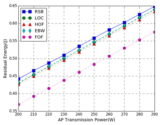
Figure 3. Residual Energy vs. Access Point (AP) Transmission Power.

Figure 4 shows the residual energy of the WP-MEC system versus the number of task-input bits. In the figure, T = 3 s, the AP transmission power is 200 W, and the number of task-input bits varies from 80 KB to 170 KB. The simulation result shows that the proposed joint optimization algorithm provides higher energy efficiency than LOC, HOF, EBW, and FOF benchmark schemes. Furthermore, the residual energy of all schemes decreases as the number of task-input bits increases. This is because the more the system tasks are executed, the higher the energy consumption will be. Accordingly, the residual energy of the system shows a downward trend as the number of task input bits increase. It is worth noting that when the number of task input bits is small, the energy efficiency of our optimization scheme is similar to LOC and EBW. As the number of task-input bits increases, the benefits of the RSB method gradually become apparent, which means our algorithm can adapt to larger computation tasks than other algorithms. It is also noticed that when the number of task-input bits is 80 KB–100 KB, the residual energy of the RSB scheme is close to EBW, indicating that in this case, the bandwidth setting of the joint optimization scheme is close to equal division. It can also be observed that the HOF curve declines slowly, indicating that the half offloading scheme is also more suitable for larger computation tasks.

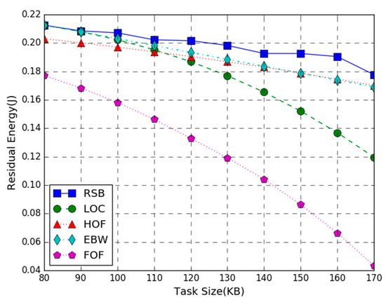
Figure 4. Residual Energy vs. Task Size.

Figure 5 shows the residual energy of the WP-MEC system versus time block length T. In the figure, the AP transmission power is 200 W, the number of the task input bits follows the uniform in the range of 80 to 100 KB, and the time block length T varies from 1.6 to 3.2 s. The simulation result shows that the proposed joint optimization algorithm provides larger residual energy than the other four schemes. Besides, as the time block length T increases, the residual energy of all schemes increases. This is because the larger the time block length T, the more energy each mobile device harvests, and the energy consumption of task computing decreases. Hence, the residual energy shows an upward trend. It is worth noting that when the length of the time block T is smaller, the difference of maximum residual energy between the RSB scheme and the other four benchmark schemes is larger. As the length of the time block increases, this difference between them gradually decreases. This result indicates that our joint optimization scheme is more suitable for the settings with the smaller time block length. It is also noticed that when the time block T is smaller, the maximum residual energy difference between the proposed joint optimization scheme and the LOC method is larger. As the time block length increases, the energy efficiency difference between RSB and LOC gradually decreases. This is because the local computing CPU frequency is affected by the time block length T. The smaller the CPU frequency of each the mobile device cycle, the lower the local computing energy consumption will be. It can also be observed that when the time block length is larger, the residual energy of EBW is closer to RSB, indicating that the equal bandwidth allocation scheme is closer to the optimal solution.

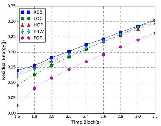
Figure 5. Residual Energy vs. Time Block.

5.3. Performance of Algorithm

The simulations in this section verify the efficiency of the proposed algorithm in solving the residual energy maximization problem in this paper. We use the PyOpt optimization tool package to solve the primary nonconvex problem. To this end, the following two benchmark schemes are used for comparing the proposed method.

Non Sorting Genetic Algorithm II (NSGA2): This algorithm can solve nonsmooth and nonconvex single and multiobjective optimization problems based on nondominating sorting genetic algorithm. When solving more complex combinatorial optimization problems, compared with some conventional optimization algorithms, this algorithm can usually obtain better optimization results faster. We adopt the NSAG2 method to solve the problem P1 directly.

Feasible Direction Method (CONMIN): The feasible direction method is a representative direct exploration method for solving constrained nonlinear optimization problems through gradients, and it is also one of the main methods for solving large-scale constrained optimization design problems. We adopt the CONMIN method to solve problem P3.

In the simulation, we test the performance of RSB, NSGA2, and CONMIN on solving the residual energy maximization problem in this paper. In order to test the performance of the algorithm from various aspects, we consider the following influencing factors in the experiment: the AP transmission power, the task size, and the time block length.

In Figure 6, the performance comparison of the residual energy maximization problem achieved by three methods in the AP transmit power varies from 200 to 290 W has been evaluated. From Figure 6a, we can see that as the AP transmit power increases, the residual energy of the three methods increases. This is because as the power of the AP increases, the energy harvesting by the mobile device increases, and the energy consumption remains unchanged. The results show that the three strategies have successfully solved the objective function, and the three algorithms are all feasible in solving the objective problem. The energy efficiency of the proposed RSB algorithm outperforms NSGA2 and CONMIN, and the residual energy is increased by 8% and 40%, respectively. This is because we get an approximate optimal solution by adopting NSGA2 to solve the primary nonconvex problem P1, while the proposed algorithm linearizes the problem P1 by RLT technology to obtain the convex problem P3 and adopts convex optimization theory to simplify the primary problem which is closer to the optimal solution of the primary problem. From the figure, the maximum residual energy difference between RSB and CONMIN is large. This is because our algorithm reduces variables, reduces computation complexity, and improves computation efficiency.

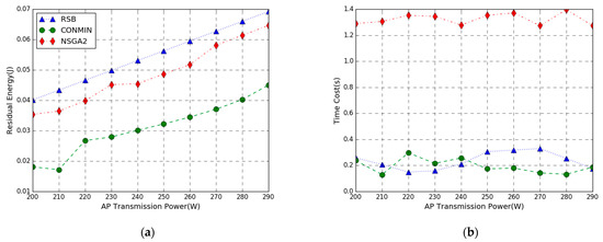
Figure 6. Performance vs. AP Transmission Power. (a) Residual Energy; (b) Time Cost.

In Figure 7, the performance comparison of the residual energy maximization problem achieved by three methods in the task input bits varies from 80 to 170 KB. The simulation result shows the residual energy of the three algorithms decrease as the number of task-input bits increases. This is because the more the number of local and offloading tasks are executed, the higher the energy consumption will be. Therefore, the residual energy of the system shows a downward trend as the number of task-input bits increases. Figure 7a shows that when the number of task input bits is smaller, the maximum residual energy difference among RSB, NSGA, and CONMIN to execute the computation task is smaller. As the number of task-input bits increases, the performance of our algorithm declines slowly, indicating that it is more suitable for larger computation tasks. It can also be observed that the residual energy curve of the NSGA2 algorithm also declines slowly. This is because the NSGA2 algorithm performs global optimization and it is easier to find a suboptimal solution close to the optimal solution.

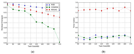
Figure 7. Performance vs. Task Size. (a) Residual Energy; (b) Time Cost.

In Figure 8, the performance comparison of the residual energy maximization problem achieved by three methods varies from 1.6 to 3.2 s. Figure 8a shows that the RSB algorithm provides a larger residual energy than the other two algorithms. As the time block length T increases, the residual energy of three algorithms increases. This is because the larger the time block length T, the more energy each mobile device harvests, and the energy consumption of local computing decreases. Accordingly, the residual energy shows an upward trend. When the time block length T is smaller, the energy efficiency of the proposed RSB algorithm outperforms NSGA2 and CONMIN. As the time block length T increases, the performance difference between the three algorithms tends to become small, indicating that our algorithm is more suitable for shorter time block length T. It can also be observed that the CONMIN algorithm consumes more energy to solve the objective function, indicating that efficiency of the algorithm is lower.

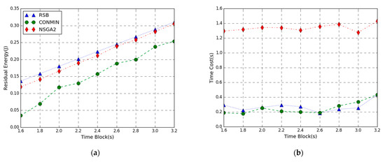
Figure 8. Performance vs. AP Time Block. (a) Residual Energy; (b) Time Cost.

From Figure 6b, Figure 7b and Figure 8b, we can see that the execution time of the RSB algorithm and CONMIN algorithm is significantly lower than the NSGA2 algorithm. This is because the nonconvex problem solved by the NSGA2 algorithm has high computation complexity and long latency. The convex problem solved by our RSB algorithm and CONMIN algorithm has higher execution efficiency. Furthermore, it can also be observed that the residual energy of our algorithm to solve the problem in this paper is much larger than the CONMIN algorithm. The above figures verify that the proposed RSB algorithm can achieve a better solution and can guarantee lower time overhead.

6. Conclusions

In this paper, we study the residual energy maximization problem at a WP-MEC system in FDMA offloading manner. By jointly optimizing the number of offloading bits, energy harvesting time, and the transmission bandwidth of mobile device, we aim to maximize residual energy by studying multiuser dynamic joint optimization of computation and wireless resource allocation under multiple time blocks. To solve this problem, we adopt convex optimization technology, combine with KKT conditions, and finally transform the problem into a univariate constrained convex optimization problem, aiming at obtaining lower time cost and higher accuracy. Furthermore, in order to improve the efficiency of solving the problem, we propose a combined method of Bisection method and sequential unconstrained minimization based on RLT. The simulation results show that our joint optimization scheme outperforms the other benchmark schemes. Moreover, the algorithm can maximize the residual energy, reduce the computation complexity, and improve computation efficiency. It is worth noting that compared with other work to maximize the residual energy, our work increases the possibility of the practical implementation of the WPT-MEC system. In the future, we will experiment in the real environment. We will simulate the wireless charging environment based on existing wireless charging devices, such as Xiaomi, Apple, and Samsung to verify the effectiveness of the proposed scheme in this paper. Besides, we will explore more efficient algorithms to build an energy efficient MEC system.

References

- Sun, X.; Ansari, N. EdgeIoT: Mobile Edge Computing for the Internet of Things. IEEE Commun. Mag. 2016, 54, 22–29. [Google Scholar] [CrossRef]
- Raj, K.; Sakshi, K.; Naveen, C. Energy conscious multi-site computation offloading for mobile cloud computing. Soft Comput. 2018, 22, 6751–6764. [Google Scholar]
- Zheng, J.; Cai, Y.; Wu, Y.; Shen, X. Dynamic Computation Offloading for Mobile Cloud Computing: A Stochastic Game-Theoretic Approach. IEEE Trans. Mob. Comput. 2019, 18, 771–786. [Google Scholar] [CrossRef]
- De, D.; Mukherjee, A.; Roy, D.G. Power and Delay Efficient Multilevel Offloading Strategies for Mobile Cloud Computing. Wirel. Pers. Commun. 2020, 112, 2159–2186. [Google Scholar] [CrossRef]
- Baktir, A.C.; Ozgovde, A.; Ersoy, C. How Can Edge Computing Benefit from Software-Defined Networking: A Survey, Use Cases & Future Directions. IEEE Commun. Surv. Tutor. 2017, 19, 2359–2391. [Google Scholar]
- Wu, H.; Tian, H.; Nie, G.; Zhao, P. Wireless Powered Mobile Edge Computing for Industrial Internet of Things Systems. IEEE Access 2020, 8, 101539–101549. [Google Scholar] [CrossRef]
- Janatian, N.; Stupia, I.; Vandendorpe, L. Optimal Offloading Strategy and Resource Allocation in SWIPT-based Mobile-Edge Computing Networks. In Proceedings of the 2018 15th International Symposium on Wireless Communication Systems (ISWCS), Lisbon, Portugal, 28–31 August 2018. [Google Scholar]
- Asiedu, D.K.P.; Mahama, S.; Song, C.; Kim, D.; Lee, K.J. Beamforming and Resource Allocation for Multi-User Full-Duplex Wireless Powered Communications in IoT Networks. IEEE Internet Things J. 2020, 7, 11355–11370. [Google Scholar] [CrossRef]
- Hu, X.; Wong, K.K.; Yang, K. Wireless Powered Cooperation-Assisted Mobile Edge Computing. IEEE Trans. Wirel. Commun. 2018, 17, 2375–2388. [Google Scholar] [CrossRef]
- Kumar, K.; Lu, Y.H. Cloud Computing for Mobile Users: Can Offloading Computation Save Energy? Computer 2010, 43, 51–56. [Google Scholar] [CrossRef]
- Cuervo, E.; Balasubramanian, A.; Cho, D.K.; Wolman, A.; Bahl, P. MAUI: Making smartphones last longer with code offload. In Proceedings of the 8th International Conference on Mobile Systems, Applications, and Services, San Francisco, CA, USA, 14–18 June 2010. [Google Scholar]
- Kosta, S.; Aucinas, A.; Hui, P.; Mortier, R.; Zhang, X. ThinkAir: Dynamic resource allocation and parallel execution in the cloud for mobile code offloading. In Proceedings of the IEEE INFOCOM 2012, Orlando, FL, USA, 25–30 March 2012; pp. 945–953. [Google Scholar]
- Yang, L.; Xu, G.; Ge, J.; Liu, P.; Fu, X. Energy-Efficient Resource Allocation for Application Including Dependent Tasks in Mobile Edge Computing. KSII Trans. Internet Inf. Syst. 2020, 14, 2422–2443. [Google Scholar]
- Li, Y.; Xu, G.; Yang, K.; Ge, J.; Jin, Z. Energy Efficient Relay Selection and Resource Allocation in D2D-Enabled Mobile Edge Computing. IEEE Trans. Veh. Technol. 2020, 69, 15800–15814. [Google Scholar] [CrossRef]
- Mao, Y.; You, C.; Zhang, J.; Huang, K.; Letaief, K.B. A Survey on Mobile Edge Computing: The Communication Perspective. IEEE Commun. Surv. Tutor. 2017, 19, 2322–2358. [Google Scholar] [CrossRef]
- Zhou, F.; Wu, Y.; Hu, R.Q.; Qian, Y. Computation Rate Maximization in UAV-Enabled Wireless-Powered Mobile-Edge Computing Systems. IEEE J. Sel. Areas Commun. 2018, 36, 1927–1941. [Google Scholar] [CrossRef]
- Habiba, U.; Maghsudi, S.; Hossain, E. A Reverse Auction Model for Efficient Resource Allocation in Mobile Edge Computation Offloading. In Proceedings of the 2019 IEEE Global Communications Conference (GLOBECOM), Waikoloa, HI, USA, 9–13 December 2019. [Google Scholar]
- Liu, M.; Liu, Y. Price-Based Distributed Offloading for Mobile-Edge Computing With Computation Capacity Constraints. IEEE Wirel. Commun. Lett. 2017, 7, 420–423. [Google Scholar] [CrossRef]
- Wang, Y.; Sheng, M.; Wang, X.; Wang, L.; Li, J. Mobile-Edge Computing: Partial Computation Offloading Using Dynamic Voltage Scaling. IEEE Trans. Commun. 2016, 64, 4268–4282. [Google Scholar] [CrossRef]
- Mao, Y.; Zhang, J.; Letaief, K.B. Dynamic Computation Offloading for Mobile-Edge Computing with Energy Harvesting Devices. IEEE J. Sel. Areas Commun. 2016, 34, 3590–3605. [Google Scholar] [CrossRef]
- Li, X.; Fan, R.; Hu, H.; Zhang, N.; Chen, X. Energy-efficient Resource Allocation for Mobile Edge Computing Aided by Multiple Relays. 2020. Available online: https://arxiv.org/pdf/2004.03821.pdf (accessed on 11 March 2021).
- You, C.; Huang, K.; Chae, H.; Kim, B.H. Energy-Efficient Resource Allocation for Mobile-Edge Computation Offloading. IEEE Trans. Wirel. Commun. 2017, 16, 1397–1411. [Google Scholar] [CrossRef]
- Feng, H.; Guo, S.; Zhu, A.; Wang, Q.; Liu, D. Energy-efficient User Selection and Resource Allocation in Mobile Edge Computing. Ad Hoc Netw. 2020, 107, 102202. [Google Scholar] [CrossRef]
- Li, X.; Guo, S.; Li, P. Energy-Efficient Data Collection Scheme Based on Mobile Edge Computing in WSNs. In Proceedings of the 2019 15th International Conference on Mobile Ad-Hoc and Sensor Networks (MSN), Shenzhen, China, 11–13 December 2019. [Google Scholar]
- Zhao, T.; Zhou, S.; Song, L.; Jiang, Z.; Guo, X.; Niu, Z. Energy-optimal and delay-bounded computation offloading in mobile edge computing with heterogeneous clouds. China Commun. 2020, 17, 191–210. [Google Scholar] [CrossRef]
- Wang, X.; Giannakis, G.B. Power-Efficient Resource Allocation for Time-Division Multiple Access Over Fading Channels. IEEE Trans. Inf. Theory 2008, 54, 1225–1240. [Google Scholar] [CrossRef]
- Wong, C.Y.; Cheng, R.S.; Lataief, K.B.; Murch, R.D. Multiuser OFDM with adaptive subcarrier, bit, and power allocation. IEEE J. Sel. Areas Commun 1999, 17, 1747–1758. [Google Scholar] [CrossRef]
- Oh, S.J.; Zhang, D.; Wasserman, K.M. Optimal resource allocation in multiservice CDMA networks. IEEE Trans. Wirel. Commun. 2003, 2, 811–821. [Google Scholar]
- Chen, J.; Xing, H.; Lin, X.; Bi, S. Joint Cache Placement and Bandwidth Allocation for FDMA-based Mobile Edge Computing Systems. In Proceedings of the ICC 2020—2020 IEEE International Conference on Communications (ICC), Dublin, Ireland, 7–11 June 2020. [Google Scholar]
- Zhang, K.; Mao, Y.; Leng, S.; Zhao, Q.; Li, L.; Peng, X.; Pan, L.; Maharjan, S.; Zhang, Y. Energy-Efficient Offloading for Mobile Edge Computing in 5G Heterogeneous Networks. IEEE Access 2016, 4, 5896–5907. [Google Scholar] [CrossRef]
- Wang, F.; Xu, J.; Wang, X.; Cui, S. Joint Offloading and Computing Optimization in Wireless Powered Mobile-Edge Computing Systems. In Proceedings of the 2017 IEEE International Conference on Communications (ICC), Paris, France, 21–25 May 2017. [Google Scholar]
- Le, H.Q.; Al-Shatri, H.; Klein, A. Efficient resource allocation in mobile-edge computation offloading: Completion time minimization. In Proceedings of the 2017 IEEE International Symposium on Information Theory (ISIT), Aachen, Germany, 25–30 June 2017. [Google Scholar]
- Liu, B.; Wang, J.; Ma, S.; Zhou, F.; Ma, Y.; Lu, G. Energy-Efficient Cooperation in Mobile Edge Computing-Enabled Cognitive Radio Networks. IEEE Access 2019, 7, 45382–45394. [Google Scholar] [CrossRef]
- Mahmood, A.; Ahmed, A.; Naeem, M.; Hong, Y. Partial Offloading in Energy Harvested Mobile Edge Computing: A Direct Search Approach. IEEE Access 2020, 8, 36757–36763. [Google Scholar] [CrossRef]
- Zhao, P.; Tao, J.; Rauf, A.; Jia, F.; Longting, X.U. Load Balancing for Energy-Harvesting Mobile Edge Computing. IEICE Trans. Fundam. Electron. Commun. Comput. Sci. 2020, E104.A, 336–342. [Google Scholar] [CrossRef]
- Liu, P.; Xu, G.; Yang, K.; Wang, K.; Li, Y. Joint Optimization for Residual Energy Maximization in Wireless Powered Mobile-Edge Computing Systems. KSII Trans. Internet Inf. Syst. 2018, 12, 5614–5633. [Google Scholar]
- Li, L.; Xu, G.; Liu, P.; Li, Y.; Ge, J. Jointly Optimize the Residual Energy of Multiple Mobile Devices in the MEC–WPT System. Future Internet 2020, 12, 233. [Google Scholar] [CrossRef]
- Wang, F.; Xing, H.; Xu, J. Real-Time Resource Allocation for Wireless Powered Multiuser Mobile Edge Computing With Energy and Task Causality. IEEE Trans. Commun. 2020, 68, 7140–7155. [Google Scholar] [CrossRef]
- Ding, J.; Jiang, L.; He, C. User-centric Energy-efficient Resource Management for Time Switching Wireless Powered Communications. IEEE Commun. Lett. 2017, 22, 165–168. [Google Scholar] [CrossRef]
- Kim, B.; Kang, J.M.; Kim, H.M.; Lee, J. Energy efficiency optimization in multi-antenna wireless powered communication network. In Proceedings of the 2016 International Conference on Information and Communication Technology Convergence (ICTC), Jeju Island, Korea, 19–21 October 2016. [Google Scholar]
- Lyu, B.; Yang, Z.; Gui, G.; Sari, H. Optimal Time Allocation in Backscatter Assisted Wireless Powered Communication Networks. Sensors 2017, 17, 1258. [Google Scholar]
- Wang, F.; Xu, J.; Cui, S. Optimal Energy Allocation and Task Offloading Policy for Wireless Powered Mobile Edge Computing Systems. IEEE Trans. Wirel. Commun. 2020, 19, 2443–2459. [Google Scholar] [CrossRef]
- Lu, W.; Xu, X.; Lu, F.; Peng, H.; Gong, Y. Resource optimization in anti-interference UAV powered cooperative mobile edge computing network. Phys. Commun. 2020, 42, 101128. [Google Scholar] [CrossRef]
- Wu, Q.; Tao, M.; Ng, D.W.K.; Chen, W.; Schober, R. Energy-Efficient Resource Allocation for Wireless Powered Communication Networks. IEEE Trans. Wirel. Commun. 2015, 15, 2312–2327. [Google Scholar] [CrossRef]
- Zhang, W.; Wen, Y.; Guan, K.; Kilper, D. Energy-Optimal Mobile Cloud Computing under Stochastic Wireless Channel. IEEE Trans. Wirel. Commun. 2013, 12, 4569–4581. [Google Scholar] [CrossRef]
- Perez, R.E.; Jansen, P.W.; Martins, J.R.R.A. pyOpt: A Python-based object-oriented framework for nonlinear constrained optimization. Struct. Multidiscip. Optim. 2012, 45, 101–118. [Google Scholar] [CrossRef]
Publisher’s Note: MDPI stays neutral with regard to jurisdictional claims in published maps and institutional affiliations. |
© 2021 by the authors. Licensee MDPI, Basel, Switzerland. This article is an open access article distributed under the terms and conditions of the Creative Commons Attribution (CC BY) license (http://creativecommons.org/licenses/by/4.0/).