Forest Parameter Prediction Using an Image-Based Point Cloud: A Comparison of Semi-ITC with ABA

Abstract

Image-based point clouds obtained using aerial photogrammetry share many characteristics with point clouds obtained by airborne laser scanning (ALS). Two approaches have been used to predict forest parameters from ALS: the area-based approach (ABA) and the individual tree crown (ITC) approach. In this article, we apply the semi-ITC approach, a variety of the ITC approach, on an image-based point cloud to predict forest parameters and compare the performance to the ABA. Norwegian National Forest Inventory sample plots on a site in southeastern Norway were used as the reference data. Tree crown objects were delineated using a watershed segmentation algorithm, and explanatory variables were calculated for each tree crown segment. A multivariate kNN model for timber volume, stem density, basal area and quadratic mean diameter with the semi-ITC approach produced RMSEs of 30%, 46%, 25%, 26%, respectively. The corresponding measures for the ABA were 30%, 51%, 26%, 35%, respectively. Univariate kNN models resulted in timber volume RMSEs of 25% for the semi-ITC approach and 22% for the ABA. A non-linear logistic regression model with the ABA produced an RMSE of 23%. Both approaches predicted timber volume with comparable precision and accuracy at the plot level. The multivariate kNN model was slightly more precise with the semi-ITC approach, while biases were larger.

1. Introduction

High resolution, three-dimensional (3D) point clouds from remote sensing are valuable for forest inventories, because vegetation height is correlated to key forest parameters. In combination with field inventories, such height information can be used to create resource maps or to estimate forest variables for small areas [1,2]. Currently, the most prominent method of acquiring point clouds is airborne laser scanning (ALS).

Remote sensing data, which increasingly attracts attention in forest inventory research, are image-based point clouds from digital aerial photogrammetry [3,4,5,6]. Advances in image quality, algorithms and computing power allow the creation of height information over large areas with high spatial resolution from images of aerial photographic surveys. Image-based point clouds and canopy height models (CHM) provide less structural information of the canopy than ALS, but can be equally accurate for predicting timber volume [7,8,9].

Two approaches have been used to estimate forest parameters from ALS. The area-based approach (ABA) uses ALS height distribution metrics of the entire plot as input to a statistical model for forest parameters, such as timber volume [10]. Individual tree crown (ITC) approaches, on the other hand, produce predictions for tree crown objects. Tree crowns are delineated from the remote sensing data by using segmentation algorithms, e.g., [11,12,13]. One approach, that corrects for biases due to segmentation errors, is the semi-individual tree crown (semi-ITC) approach [14]. The difference of semi-ITC from other ITC approaches is that crown segments can contain none, one or several trees. While often not resulting in higher accuracies than using the ABA [15], ITC approaches can be attractive for forest owners because of their higher spatial resolution.

Most studies using image-based point clouds for forest parameter prediction apply the ABA. Only one study applied the semi-ITC approach on an image-based CHM [16], but focused on tree height estimation and used a coarse resolution of 4 m × 4 m. The objective of this study was to apply the semi-ITC approach on a very high resolution (15.6 points·m${}^{-2}$) image-based point cloud to predict timber volume, stem density, basal area (G) and the quadratic mean diameter (QMD). The performance of the semi-ITC approach was compared to the ABA.

2. Material and Methods

2.1. Study Area

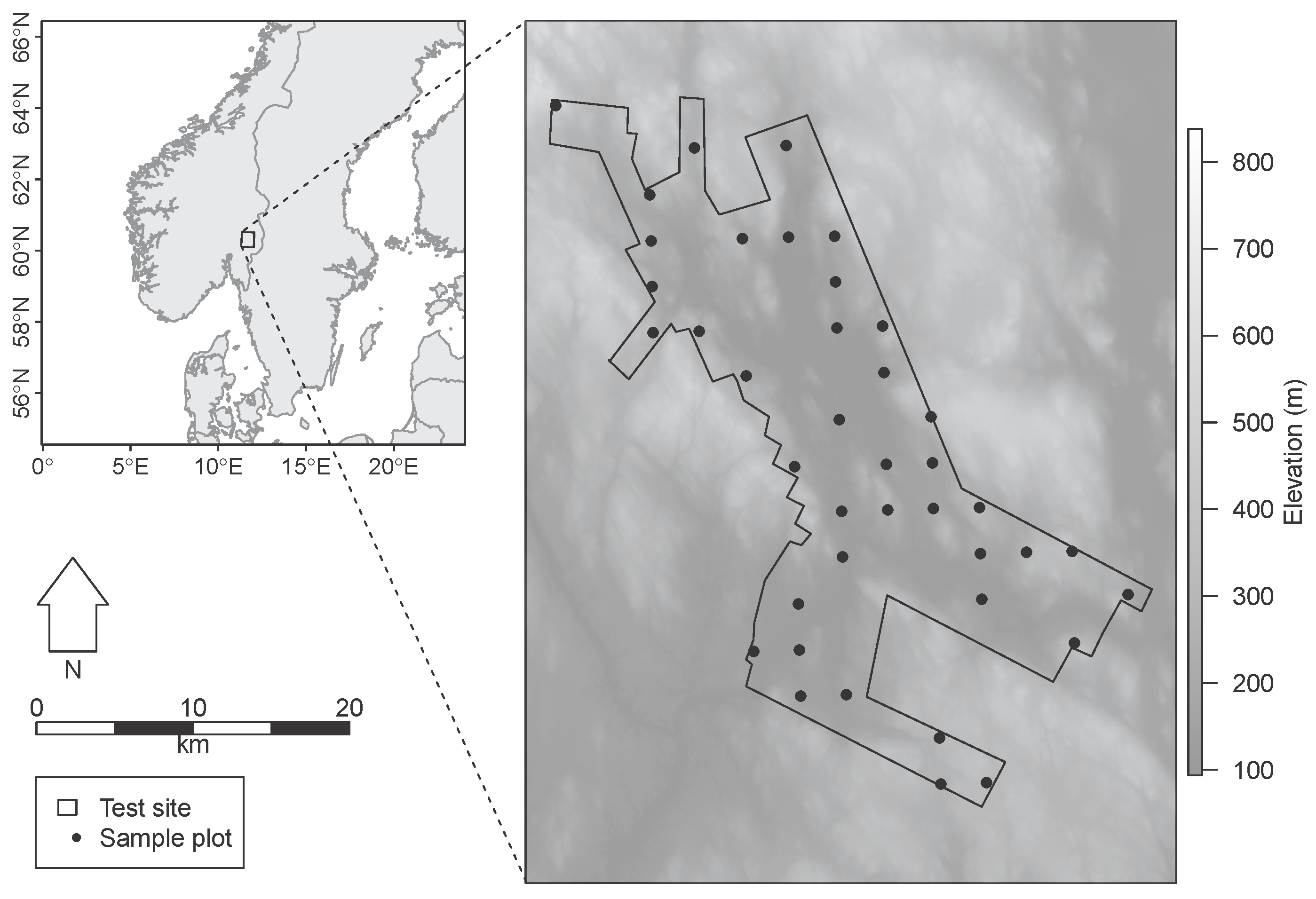
The study area is located in Hedmark county in southeastern Norway. It covers parts of the municipalities Nord-Odal, Sør-Odal and Kongsvinger. The boreal forest is dominated by Norway spruce (Picea abies (L.) Karst.) and includes Scots pine (Pinus sylvestris L.), birch (Betula spp.) and small portions of other tree species, such as aspen (Populus tremula L.) and rowan (Sorbus aucuparia L.). The terrain is hilly with altitudes ranging from 130 to 535 m a.s.l (Figure 1).

Figure 1. Overview of the study area with a standard Norwegian DTM in the background.

Figure 1. Overview of the study area with a standard Norwegian DTM in the background.

2.2. Field Data

The field data used in this study are sample plots of the Norwegian National Forest Inventory (NFI). The plots were located on a 3 km × 3 km grid. Within the sample plot radius of 8.92 m (250 m${}^2$), the recorded variables include species, tree positions, diameter at breast height (dbh) of all trees with dbh >5 cm and tree height measured with a Vertex hypsometer. On sample plots with 10 or less trees, the heights of all trees are measured. On plots with more than 10 trees, a sub-sample is selected using a relascope. The relascope factor for the selection is calculated on site for each sample plot to achieve a sub-sample size of approximately 10 trees. The height of trees without height measurement is estimated with dbh height models derived from trees having height measurements [17]. Timber volume for each tree is estimated with species-specific allometric models [18,19,20].

A total of 44 NFI sample plots were located within the study area. Four plots were discarded due to harvesting between the image acquisition and the field inventory. The NFI plots were measured between 2008 and 2012. An accurate positioning of the plots was achieved using differential GPS. Descriptive statistics of the forest inventory data can be found in Table 1.

Table 1. Descriptive statistics of the 40 National Forest Inventory (NFI) plots.

Variable	Min	Mean	Max	SD
Total volume (m${}^3$·ha${}^{-1}$)	3	199	459	142
Spruce volume (m${}^3$·ha${}^{-1}$)	0	121	445	135
Pine volume (m${}^3$·ha${}^{-1}$)	0	45	382	81
Deciduous species volume (m${}^3$·ha${}^{-1}$)	0	33	198	48
Basal area (m${}^2$·ha${}^{-1}$)	1	23	49	14
Quadratic mean diameter (cm)	7	16	39	6
Stem density (ha${}^{-1}$)	40	1332	4520	909

Table 1. Descriptive statistics of the 40 National Forest Inventory (NFI) plots.

Variable	Min	Mean	Max	SD
Total volume (m${}^3$·ha${}^{-1}$)	3	199	459	142
Spruce volume (m${}^3$·ha${}^{-1}$)	0	121	445	135
Pine volume (m${}^3$·ha${}^{-1}$)	0	45	382	81
Deciduous species volume (m${}^3$·ha${}^{-1}$)	0	33	198	48
Basal area (m${}^2$·ha${}^{-1}$)	1	23	49	14
Quadratic mean diameter (cm)	7	16	39	6
Stem density (ha${}^{-1}$)	40	1332	4520	909

2.3. Image-Based Point Cloud

A Vexcel Ultracam Eagle camera was used to acquire the images on 11 May 2010. The image ground sampling distance (resolution) was 10 cm. A total of 1024 images covered the study area.

The stereo matching of the aerial images was conducted by an external vendor, Blom AS, Norway. The software used for matching was Match-T Version 5.5.2. with the “mountainous” matching strategy. Corresponding heights of a digital terrain model (DTM) obtained from airborne laser scanning were subtracted from the point cloud z-coordinate to extract the vegetation heights. The point density was 15.6 points·m${}^{-2}$. The points were assigned RGB color values from the corresponding pixel of the aerial image with the closest center point.

2.4. ALS Data

We generated a digital terrain model (DTM) from ALS data acquired in 2009 and 2010. The mean pulse density was 1.2 m${}^{-2}$, and each echo was classified as ground and non-ground by the vendor. The DTM had a cell size of 0.5 m × 0.5 m, and the terrain elevation was derived as the mean height of the ground echoes within each cell. The elevation of cells containing no echoes was interpolated by inverse distance weighting the closest data cells in each of the eight directions of the raster (orthogonal and diagonal) [21].

2.5. Semi-ITC Approach

For the tree crown segmentation, we created a canopy height model (CHM) with a pixel size of 0.5 m × 0.5 m using the highest point within each cell. No-data cells caused by missing points in the point cloud were interpolated by inverse distance weighting the closest data cells in each of the eight directions of the raster (orthogonal and diagonal).

We used a watershed algorithm [22] to segment crown outlines based on the CHMs. A threshold of 2 m was applied to separate ground and low vegetation from areas covered by trees. These areas were segmented in two different ways. Above 2 m, we set the height tolerance of the algorithm to 10 cm. The height tolerance is the minimum height between the highest point of a segment and all of its border pixels. If a segment has a minimum height smaller than the tolerance, the segment is merged with the highest neighboring segment. In this way, small maxima, which occur often in the CHM, are ignored. Below 2 m, the tolerance was set to 5 cm to reduce the size of the segments. All segments smaller than 2 m${}^2$ were discarded, and each of their pixels was assigned to the closest neighboring segment.

In earlier studies applying the semi-ITC approach to ALS, e.g., [15], the segmentation resulted in segments covering only the parts of the plot where tree crowns were detected. Treeless areas were therefore ignored in the statistical modeling. In this study, the sample plot area was completely covered by segments. Such coverage was desired to avoid omission errors, since single tree crowns were occasionally invisible in the point cloud.

Based on the field inventory data, timber volume, G and the quadratic diameter of all trees within each segment were summed. The parameters of segments without trees were set to 0. For the statistical modeling, the segments were classified in reference and target segments. Reference segments were all segments lying completely within the sample plots and were used as training data to fit the statistical models. Target segments were segments partly intersecting with the sample plot, for which the response variables were only predicted with the fitted models.

For each segment, height-distribution metrics were calculated from the image-based point cloud using FUSION [21]. The height metrics were minimum ($H_{min}$), mean ($H_{mean}$), maximum ($H_{max}$) and the standard deviation ($H_{sd}$) of the point heights, as well as the 1%, 5%, 10%, 20%, 25%, 30%, 40%, 50%, 60%, 70%, 75%, 80%, 90%, 95% and 99% height percentiles ($H_{P01}$,…,$H_{P99}$). Density metrics were derived by dividing the vertical distance between the lowest and the highest point within each segment into ten equal sections and calculating the proportion of the number of points within each section to the total number of points in the segment ($D_1$,…,$D_{10}$) [23]. Color metrics, i.e., radiometric distribution metrics, which describe the distribution of the numeric color values, were derived similarly to the height metrics for each color band ($R_{min}$, $R_{mean}$, $R_{max}$, $R_{sd}$, $R_{P01}$,…,$R_{P99}$, $G_{min}$, $G_{mean}$, $G_{max}$, $G_{sd}$, $G_{P01}$,…,$G_{P99}$, $B_{min}$, $B_{mean}$, $B_{max}$, $B_{sd}$, $B_{P01}$,…,$B_{P99}$). Ratios ($R_{ratio}$, $G_{ratio}$, $B_{ratio}$) were calculated for each color by dividing the mean color value (e.g., $G_{mean}$) by the sum of all mean color values. Additionally, geometric properties of the segments were derived, i.e., area ($Ge{o}_A$), perimeter ($Ge{o}_P$) and compactness ($Ge{o}_C=Ge{o}_A/\sqrt{Ge{o}_P}$).

2.6. Area-Based Approach

As explanatory variables for the ABA, we derived the same height, density and color metrics as for the semi-ITC approach. The metrics were calculated from point heights and colors of the entire area of each plot. Geometry metrics were not calculated, because area and shape do not differ between sample plots.

2.7. Statistical Modeling

To compare the approaches thoroughly, we fitted kNN-models for both the semi-ITC approach and the ABA: a kNN-model with multiple response variables (multivariate kNN) and a kNN model with a single response variable (univariate kNN). Additionally, we fitted a non-linear logistic regression model for the ABA, because parametric models are commonly used for the ABA.

The response variables for the kNN-model with multiple response variables were timber volume, G, QMD and stem density. For the kNN model with the single response variable, we used timber volume as the response variable. The kNN-models are based on using Euclidean distance as the distance metric and k = 1. We selected explanatory variables with the help of a forward stepwise algorithm.

We fitted a non-linear logistic regression model to the response variable timber volume for the ABA. A logistic model was preferred over a linear model, because curvilinearity was found in the data. Additionally, the model incorporates two asymptotes, which restrict possible predictions to a range between zero and an adjustable maximum value and, thus, prevent extreme predictions [24]. The model is given by:

$$y_i=\frac{\alpha }{1+exp\left({\displaystyle {\beta }_0+\sum _{j=1}^J{\beta }_j{x}_{ji}}\right)}+{\epsilon }_j$$

(1)

where $y_i$ is the prediction for the i-th plot, $x_{ij}$ is the value of the j-th explanatory variable of the i-th plot, ${\beta }_0$ and ${\beta }_j$ are the parameters to be estimated, α is the maximum asymptote and ${\epsilon }_i$ is the residual error. The best value for asymptote α was determined by an optimization algorithm set to minimize the RMSE of the cross-validated predictions. Mean elevation was used as the explanatory variable in the optimization.

Cross-validation was applied to all models to avoid overfitting. For the semi-ITC approach, the model was fitted for each plot without using the reference segments of the plot. Subsequently, the response variables were predicted for all target and reference segments within the plot. For the ABA, a leave-one-out cross-validation at the plot level was applied.

For the semi-ITC approach, plot-level predictions were derived by aggregating the segment predictions: segment predictions were multiplied by the proportion of the segment area shared with the sample plot to correct overprediction caused by segments overlapping the sample plot boundary. This correction, however, introduces an error, because it assumes homogeneity within the segments. The segment predictions of timber volume, G and stem density were then totaled at the plot level. For the QMD, the quadratic diameter was first aggregated like the other parameters and then divided by the predicted number of stems. The QMD at the plot level was the square root of this number.

We used the root mean square error (RMSE) on the plot level as the goodness-of-fit criterion. The RMSE was used as a basis for the comparison and the stepwise variable selection. RMSE on the plot and segment level was calculated as:

$$RMSE=\sqrt{\frac{{\sum }_{i=1}^n{(y_i-{\widehat{y}}_i)}^2}{n}}$$

(2)

where n is the sample size, $y_i$ is the observed forest parameter of the i-th population unit (plots or segments) and ${\widehat{y}}_i$ is the predicted forest parameter of the i-th population unit.

The RMSE in percent was calculated as:

$$RMSE(\%)=\frac{RMSE}{\overline{y}}\times 100$$

(3)

where $\overline{y}$ is the mean observed forest parameter on the plot or segment level.

To assess the systematic error of the models, we calculated the bias as:

$$BIAS=\frac{{\sum }_{i=1}^n{y}_i-{\widehat{y}}_i}{n}$$

(4)

3. Results

3.1. Comparison of the Two Approaches

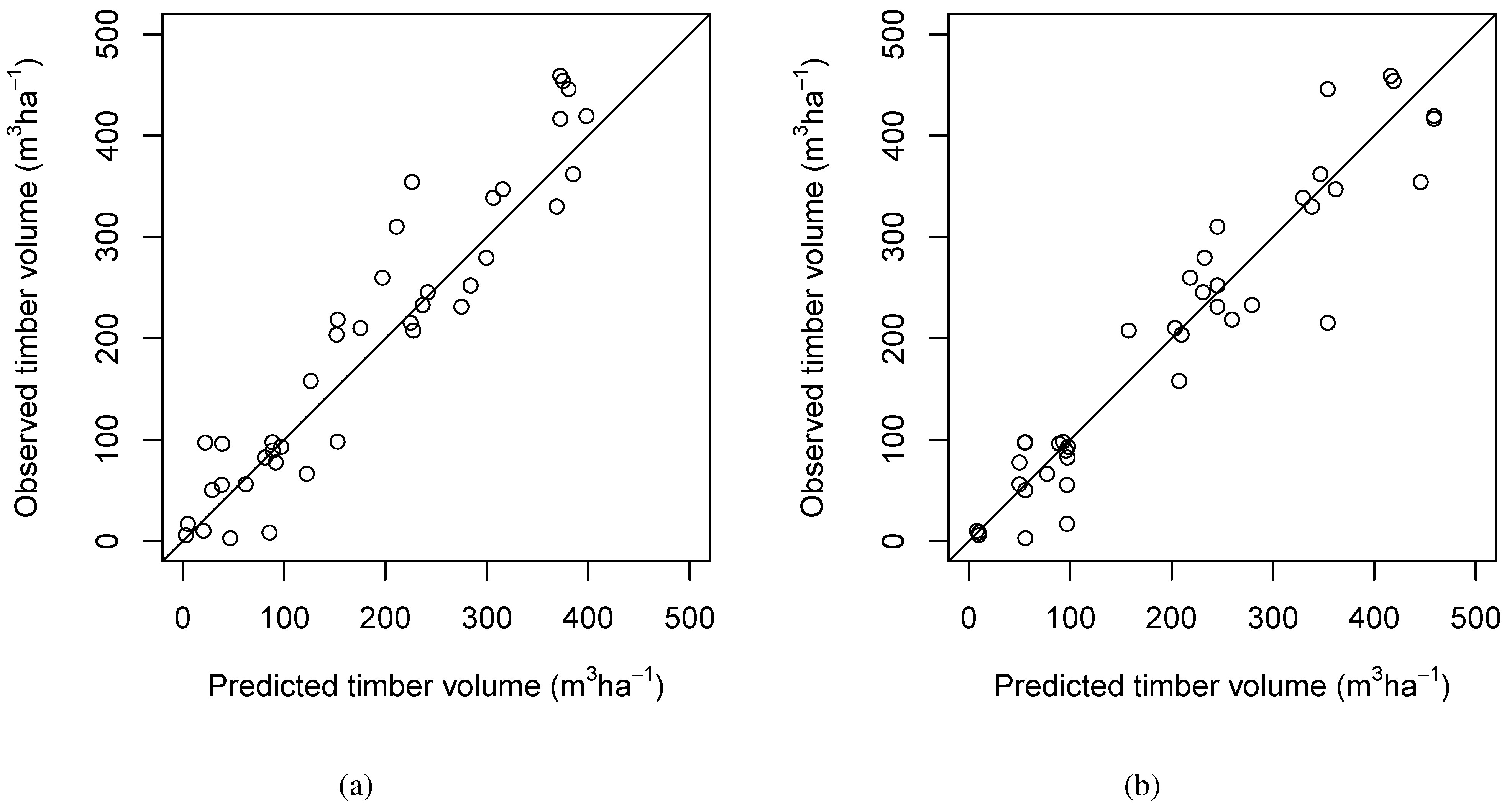
Timber volume models show a reasonably good fit with both the semi-ITC approach and the ABA. The semi-ITC univariate kNN model produced a slightly higher RMSE than the ABA univariate kNN model (Table 2). The ABA univariate kNN model was marginally better than the logistic regression model. The best volume model of each approach, which was for both approaches the univariate kNN model, is shown in Figure 2. Both univariate kNN models performed similarly. No strong indication for the heteroscedasticity of the residuals was given. A curvilinear relationship between the residuals and the observed timber volumes was not visible. None of the models produced outliers.

Table 2. RMSEs of the model predictions. G, basal area. QMD, quadratic mean diameter.

Model	Approach	Volume		Stem density		G		QMD
		m${}^3$·ha${}^{-1}$	%	ha${}^{-1}$	%	m${}^2$·ha${}^{-1}$	%	cm	%
multivariate kNN	semi-ITC	60	30	612	46	6	25	4	26
	ABA	61	30	673	51	6	26	6	35
univariate kNN	semi-ITC	51	25
	ABA	44	22
logistic regression	ABA	45	23

Table 2. RMSEs of the model predictions. G, basal area. QMD, quadratic mean diameter.

Model	Approach	Volume		Stem density		G		QMD
		m${}^3$·ha${}^{-1}$	%	ha${}^{-1}$	%	m${}^2$·ha${}^{-1}$	%	cm	%
multivariate kNN	semi-ITC	60	30	612	46	6	25	4	26
	ABA	61	30	673	51	6	26	6	35
univariate kNN	semi-ITC	51	25
	ABA	44	22
logistic regression	ABA	45	23

Figure 2. Observed versus predicted timber volume at the plot level using using (a) the semi-ITC approach and (b) the ABA.

Figure 2. Observed versus predicted timber volume at the plot level using using (a) the semi-ITC approach and (b) the ABA.

The biases of the semi-ITC models were all positive and, in absolute terms, larger than the biases of the ABA (Table 3). The smallest difference in accuracy was found between the univariate kNN models. All ABA multivariate kNN models showed a negative bias. The logistic regression model had the smallest bias.

The multivariate kNN model predictions of both approaches differ more. The semi-ITC approach performed better than or equally as good as the ABA for all forest parameters. The biggest differences can be found in the QMD and stem density predictions.

Table 3. Biases of the model predictions. G, basal area. QMD, quadratic mean diameter.

Model	Approach	Volume		Stem density		G		QMD
		m${}^3$·ha${}^{-1}$	%	ha${}^{-1}$	%	m${}^2$·ha${}^{-1}$	%	cm	%
multivariate kNN	semi-ITC	29	15	146	11	3	12	1	6
	ABA	−6	−3	−23	−2	−1	−3	0	−1
univariate kNN	semi-ITC	11	5
	ABA	−4	2
logistic regression	ABA	1	0

Table 3. Biases of the model predictions. G, basal area. QMD, quadratic mean diameter.

Model	Approach	Volume		Stem density		G		QMD
		m${}^3$·ha${}^{-1}$	%	ha${}^{-1}$	%	m${}^2$·ha${}^{-1}$	%	cm	%
multivariate kNN	semi-ITC	29	15	146	11	3	12	1	6
	ABA	−6	−3	−23	−2	−1	−3	0	−1
univariate kNN	semi-ITC	11	5
	ABA	−4	2
logistic regression	ABA	1	0

3.2. Semi-ITC Approach

The segmentation of the CHM produced 1240 segments, which intersected with the sample plots. A total of 440 segments lay completely within the sample plots and were used as reference segments. Table 4 shows the statistics describing the number of segments intersecting with the plots, the area of the segments and the aggregated tree list within each segment. Large area segments were caused by flat ground, where local maxima were below the height tolerance of the watershed algorithm.

Table 4. Statistics of segments and assigned field data.

Variable	Min	Mean	Max	SD
Segments per plot	9.00	31.00	55.00	9.00
Segment area (m${}^2$)	2.00	14.81	331.56	20.22
Number of trees	0.00	1.07	14.00	1.62
Timber volume (m${}^3$)	0.00	1.60	32.48	3.12
G (m${}^2$)	0.00	0.02	0.31	0.03
QMD (cm)	0.00	6.91	43.90	8.60

Table 4. Statistics of segments and assigned field data.

Variable	Min	Mean	Max	SD
Segments per plot	9.00	31.00	55.00	9.00
Segment area (m${}^2$)	2.00	14.81	331.56	20.22
Number of trees	0.00	1.07	14.00	1.62
Timber volume (m${}^3$)	0.00	1.60	32.48	3.12
G (m${}^2$)	0.00	0.02	0.31	0.03
QMD (cm)	0.00	6.91	43.90	8.60

Based on the result of the stepwise algorithm, we selected $H_{P01}$, $H_{P10}$, $H_{P90}$, $D_2$, $D_9$, $G_{min}$, $Ge{o}_P$ for the semi-ITC multivariate kNN model. For the semi-ITC univariate kNN model, $H_{min}$, $H_{sd}$, $H_{P99}$, $D_2$, $D_7$, $R_{min}$, $G_{P01}$, $Ge{o}_P$ were selected.

The RMSEs at the segment level of the multivariate kNN prediction were: 175% for timber volume, 149% for stem density, 160% for G and 156% for QMD. The segment level timber volume predictions of the univariate kNN model had an RMSE of 178%. For comparison, we define a null-model as a model containing only an intercept at the observed mean of the variable of interest ($\widehat{y}=\overline{y}$). The null model is created with the field data within the segments alone, and its precision serves as a threshold to assess the benefit of the statistical modeling. The RMSEs of the null models at the segment level were: 194% for timber volume, 151% for stem density, 173% for G and 124% for QMD. Except for QMD, all kNN parameter predictions at the segment level were better than the null model predictions.

3.3. ABA

For the ABA multivariate kNN model, the variables $H_{P05}$, $H_{P10}$, $H_{P25}$, $H_{P30}$, $H_{P60}$, $G_{P01}$ were selected, for the ABA univariate kNN model the variables $H_{mean}$, $H_{max}$, $H_{sd}$, $H_{P40}$, $H_{P60}$, $B_{P01}$, $B_{P25}$, $B_{30}$ and for the logistic regression model the variables $H_{30}$, $H_{90}$, $G_{P80}$. The optimal upper asymptote was at 598 m${}^3$·ha${}^{-1}$.

4. Discussion

Both the semi-ITC approach and the ABA showed a similar level of precision and accuracy at the plot level when predicting timber volume. Multivariate predictions of timber volume, stem density and G were equally or slightly more precise with the semi-ITC approach than with the ABA. QMD predictions with the semi-ITC multivariate kNN model had a higher precision.

The accuracy of the timber volume predictions is in accordance to earlier studies comparing the two approaches based on ALS data, which showed no or only slight accuracy improvements when using the semi-ITC approach over the ABA [14,15]. Although RMSE values are difficult to compare among studies covering different areas, the timber volume prediction accuracy at the plot level is within the range reported by earlier studies applying the ABA on image-based point clouds [7,25,26]. G predictions were more precise than previously reported with image-based point clouds [5,6].

Biases, however, were larger using the semi-ITC approach. The biases of the multivariate kNN models were positive when using the semi-ITC approach, thus indicating underestimation of the observed parameters. In contrast, biases of the multivariate kNN models were negative when using the ABA. Similarly, a larger positive bias with the semi-ITC approach was reported by an earlier study comparing ITC approaches and the ABA based on ALS for biomass prediction [15].

The semi-ITC predictions of timber volume, G and stem density at the segment level had an equal or slightly higher precision than the null model. Using the image-based point cloud can therefore be a beneficial prediction of certain forest parameters at the tree crown level. However, since the errors are still high, this benefit has to be carefully weighed against the costs of applying the semi-ITC approach. The aggregation to the plot level seems to balance out large parts of the errors similarly to aggregating ABA predictions to the stand level [7].

Comparing the variables, which were selected by the stepwise algorithm, shows an important difference of the two approaches. The variable size of the crown segments has to be considered when modeling forest parameters with the semi-ITC approach. Interestingly, the geometry metric segment perimeter ($Ge{o}_P$) was selected in both semi-ITC models rather than the area ($Ge{o}_A$).

Many crown segmentation algorithms have been developed for ALS, e.g., [27,28]; however, no study has yet investigated tree crown delineation with image-based point cloud data. Since no optimized segmentation algorithm for image-based 3D data exists, we chose to use a simple watershed algorithm [29], which we adjusted to the present data. Using color as an additional input could be one possibility to improve the tree crown segmentation.

Mismatches between field and remote sensing data can have a negative influence on forest parameter models. Discarding segments with mismatching data by selecting reference segments for modeling based on the correlation between field-measured tree heights and remote sensing height [14] does not necessarily improve the accuracy [15]. Similarly, also in our study, a pre-analysis showed that this method did not increase the accuracy and was therefore not used.

The study shows that the Norwegian NFI can provide suitable data for model calibration for the semi-ITC approach. Especially, timber volume was reasonably well distributed through its range. However, a forest inventory, designed specifically for model calibration, would ensure that plots were located more evenly throughout the ranges of the response variables. Furthermore, due to the low sample plot density, only a few sample plots were available in the study area. The small number of plots has to be taken into account to avoid overfitting. The semi-ITC approach is less sensitive, since the sample plots are divided into more, smaller segments, which are the reference for the statistical model. Due to the small number of sample plots, an independent validation dataset was not available. The study relies therefore on cross-validation.

We ignored measurement errors and errors introduced by allometric models. All NFI data were considered to be ground truth. Especially for small-scale predictions, as in this study, however, these errors could increase the variances of the predictions and introduce a bias [30].

Even though the model fits were reasonably good, we see possibilities for improvement in the image-based point cloud. The data were delivered as a smooth point cloud with mostly regular horizontal spacing. The point cloud depicts the general appearance of the forest, i.e., height and area, as well as large tree crowns. Some trees, however, especially in open areas, were not visible in the data. Reasons for such omissions might lie in the general problems of image matching of forests [31] and in the software internal algorithm to filter out erroneously-matched points. Additional information on the matching quality of each point or using an improved filtering algorithm, or even the raw point cloud might lead to better prediction accuracy.

Additionally, color information seems to be related to timber volume, since it improved the timber volume model of the ABA. Radiometric correction might contribute to a higher prediction accuracy, as it does for tree species classification [32].

We conclude that the semi-ITC approach based on the image-based point cloud produced timber volume predictions with precision and accuracy comparable to the ABA. Multivariate parameter prediction was equally or more precise with the semi-ITC-approach than with the ABA, but produced larger biases. Improved segmentation algorithms, adapted stereophotogrammetric processing and better color information might improve the semi-ITC approach with image-based point clouds in the future.