Article

Assessing Seasonal Concentrations of Airborne Potentially Toxic Elements in Tropical Mountain Areas in Thailand Using the Transplanted Lichen Parmotrema Tinctorum (Despr. ex Nyl.) Hale

by
Chaiwat Boonpeng
1,2,*,
Duangkamon Sangiamdee
3,
Sutatip Noikrad
2 and
Kansri Boonpragob
2
1
Department of Biology, Faculty of Science, Ramkhamhaeng University, Hua Mark, Bang Kapi, Bangkok 10240, Thailand
2
Lichen Research Unit, Department of Biology, Faculty of Science, Ramkhamhaeng University, Hua Mark, Bang Kapi, Bangkok 10240, Thailand
3
Department of Chemistry, Faculty of Science, Ramkhamhaeng University, Hua Mark, Bang Kapi, Bangkok 10240, Thailand
*
Author to whom correspondence should be addressed.
Forests 2023, 14(3), 611; https://doi.org/10.3390/f14030611
Submission received: 19 February 2023 / Revised: 14 March 2023 / Accepted: 17 March 2023 / Published: 19 March 2023
(This article belongs to the Special Issue Biomonitoring with Lichens and Mosses in Forests)

Abstract

:
The atmosphere of mountain areas may be contaminated by pollutants originating mainly from road traffic, as well as tourist and community activities within such areas. This study mainly aimed to assess the concentrations of airborne potentially toxic elements (PTEs) in two mountain areas in Thailand using lichen biomonitoring. Thalli of the lichen Parmotrema tinctorum from the relatively unpolluted area in Khao Yai National Park (KYNP) were prepared and exposed at nine sites in the KYNP and nine sites in Doi Inthanon National Park (DINP) during the rainy and dry seasons. The lichen transplants were collected and analyzed for 15 PTEs, including Al, As, Cd, Co, Cr, Cu, Fe, Mn, Mo, Ni, Pb, Sb, Ti, V, and Zn, using inductively coupled plasma-mass spectrometry. The result clearly showed that the atmosphere of many monitoring sites in both mountains were contaminated by the investigated PTEs. The contamination factors (CFs) revealed that several PTEs heavily contaminated the atmosphere at many monitoring sites. The pollution load indices (PLIs) clearly illustrated that the atmosphere of all sites had higher pollution loads in the dry season than in the rainy season, which was likely due to the higher numbers of motor vehicles and visitors. The highest pollution loads were observed at sites that had higher traffic density and human activities, including the park entrance site in the KYNP and the community site in the DINP. The lowest air pollution loads were discovered at the summit sites in both mountains. This study indicates that the atmosphere of mountain areas can be contaminated by some PTEs that are mainly produced by road traffic and local communities. It also confirms the ability of the transplanted lichen P. tinctorum to be an effective biomonitoring tool for airborne PTEs in natural environments.

1. Introduction

Mountainous areas generally have beautiful nature; high biodiversity; rare, endemic, and special species; and good air quality. These properties make them excellent locations for visiting, learning, picnics, and recreation. Several mountain sites in Thailand have been disturbed to facilitate tourism via the construction of roads, buildings, accommodations, camping grounds, and tourist spots. Tourism can contribute to air pollution in natural areas from traffic vehicles, cigarette smoking, and camping activities. Motor vehicles emit several kinds of pollutants, including nitrogen dioxide (NO2), sulfur dioxide (SO2), polycyclic aromatic hydrocarbons (PAHs), volatile organic compounds (VOCs), particulate matter (PM), and potentially toxic elements (PTEs) [1,2,3,4,5]. The term PTEs generally refers to elements that occur naturally in soil, rock, water, and air but can be toxic to living organisms (including humans) when they occur above an established threshold. Examples of PTEs are Al, As, Cd, Fe, Mn, Pb, and Zn [6,7,8,9]. These elements can originate from fossil fuel combustion, brake abrasives, clutch systems, tire wear, car engines and components, road damage, and the resuspension of soil dust. In addition, tobacco smoke contains several PTEs and many harmful chemicals that are carcinogenic to humans [10]. Camping activities such as cooking and fire building may release some PTEs. In addition, activities from nearby communities (e.g., agricultural practices) and long-range transport can also contribute to air pollution in mountain areas [11,12]. Thus, monitoring air quality in mountain areas is necessary to maintain good health and sustainable ecosystems.
Air quality monitoring in mountain areas is frequently performed using lichen biomonitoring [2,6,7,11,12,13,14,15,16,17]. This method is relatively low-cost and easier than installing air monitoring equipment, and it does not require electricity for installation, which enables it to be used in natural areas. Lichens are obligate symbiotic organisms between fungi and algae and/or cyanobacteria [18] and are recognized as great bioaccumulators of atmospheric pollutants [19,20]. They have no root system and rely largely on the air for water and minerals (including pollutants). The absence of stomata and cuticles allows atmospheric deposition to accumulate on the whole lichen surface. One lichen thallus can accumulate several kinds of pollutants, especially PTEs, which are generally not monitored at traditional air quality monitoring stations [6,7,11,21]. In a study area with no lichens or insufficient lichens, this can be overcome by the transplantation technique [5,22,23,24,25,26]. This method has advantages over the in-situ technique (using native lichens), including (i) allowing the assessment of spatial and temporal element concentrations, (ii) knowing the exposure time, and (iii) allowing air monitoring at high resolution. The foliose lichen Parmotrema tinctorum (Despr. ex Nyl.) Hale is widely distributed in tropical and temperate regions (GBIF.org). In Thailand, it is easily seen on tree bark and rocks in areas between 700 and 1500 m above sea level (asl). Its potential for use as a bioaccumulator and a biomonitor of air pollutants was confirmed by several previous studies in Thailand [27,28,29] and other countries [24,30,31,32].
Among the 129 terrestrial national parks in Thailand, Khao Yai National Park (KYNP) and Doi Inthanon National Park (DINP) are the most popular tourist destinations. The average numbers of visitors and motor vehicles from 2016 to 2019 (the years before the COVID-19 pandemic in Thailand) were highest in KYNP (1,529,121 persons/yr and 414,927 cars/yr) and second highest in DINP (843,279 persons/yr and 215,560 cars/yr) (Source: National Parks of Thailand). Air quality monitoring in national parks is scarce in Thailand. Our previous study preliminarily measured atmospheric contamination by some PTEs in the KYNP using the in-situ lichen P. tinctorum [28]; however, the study did not reveal the element concentrations across seasons, especially in the dry season, which generally has higher numbers of tourists and motor vehicles. Therefore, this study was conducted to fill this knowledge gap, which will be useful for park management to promote good health (for staff, tourists, residents), sustainable ecosystems, and the environment. This study was also conducted to achieve two of the United Nations’ sustainable development goals (SDGs), which are goals 3 (Good health and well-being) and 15 (Life on land). Therefore, the objectives of this study were (i) to assess the concentrations of airborne PTEs in the rainy and dry seasons in the tropical mountain areas at KYNP and DINP and (ii) to test the ability of the transplanted lichen P. tinctorum to be used as a biomonitor of airborne PTEs in natural areas.

2. Materials and Methods

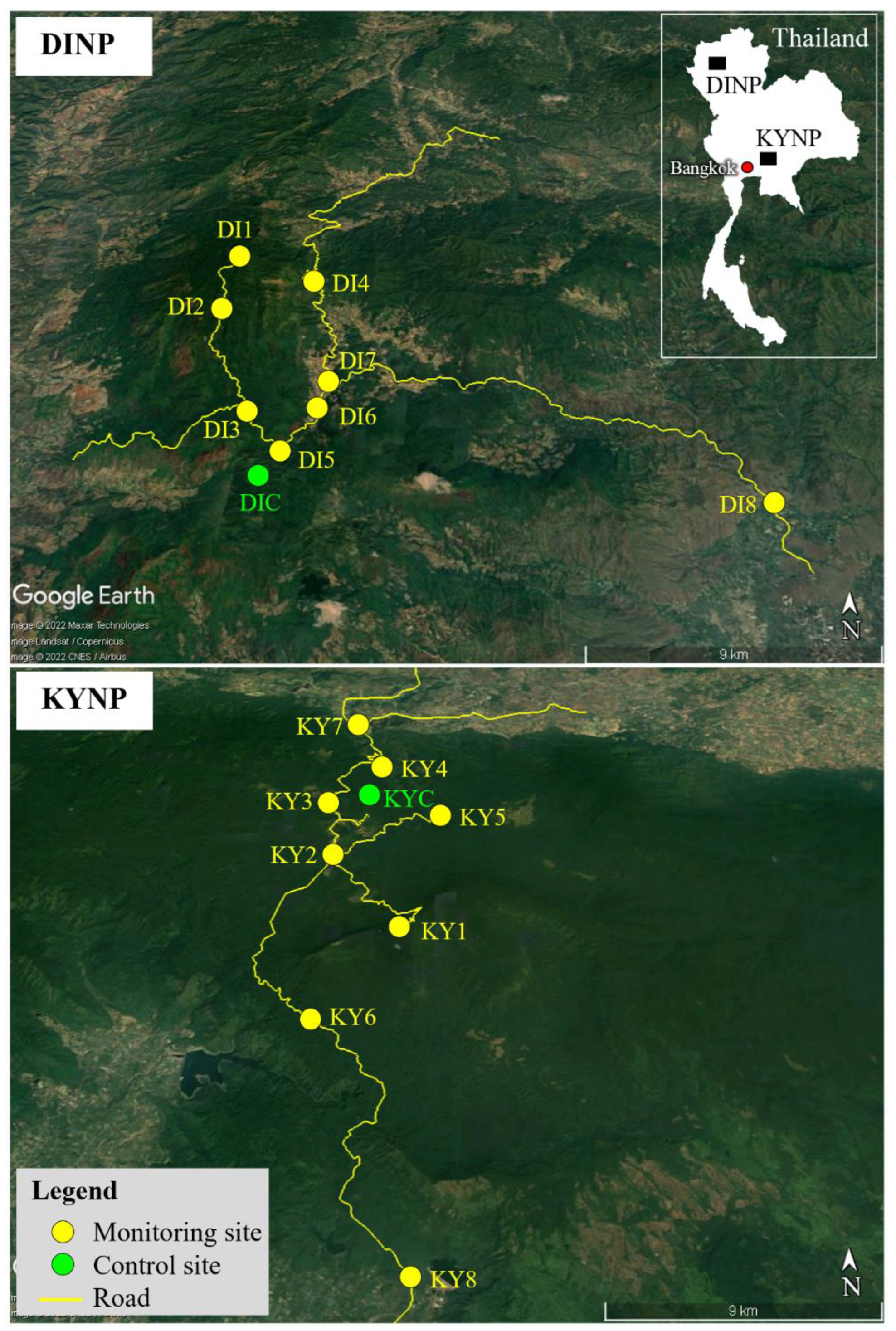
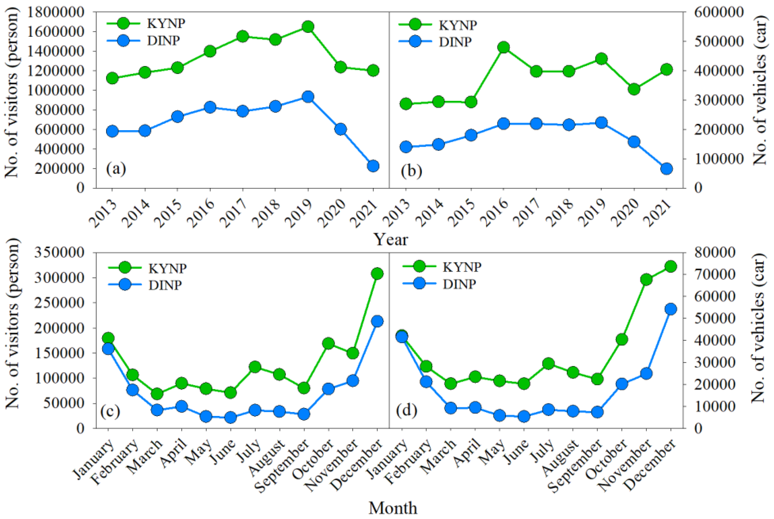
2.1. Study Area and Monitoring Site

This study was performed in two natural parks in Thailand, the KYNP and the DINP. The KYNP has an area of 2169 km2 covering parts of Prachinburi, Nakhon Ratchasima, Nakhon Nayok, and Saraburi Provinces, and it is approximately 180 km northeast of Bangkok (Figure 1). This park was established as the first national park in Thailand in 1962, and it became a UNESCO world heritage site in 2005. The terrain is made up of complex mountains with elevations ranging from approximately 50 to 1351 m asl. There is a high biodiversity of plants, animals, and fungi. Most of the area is covered by moist evergreen forest, followed by mixed deciduous forest, hill evergreen forest, dry evergreen forest, and deciduous dipterocarp forest (Source: National Parks of Thailand). The average cumulative rainfall from 1993 to 2021 (29 years) at the station near the park office (760 m asl) was 1996 mm/yr. The wet period is between May and October, when the amount of rainfall is more than 200 mm/month, while the dry period is between November and February, when the rainfall amount is less than 50 mm/month (Source: Thai Meteorological Department). The monthly average relative air humidity ranges from 68% (January) to 90% (September), while the monthly average air temperature ranges from 19 °C (December to January) to 24 °C (April to June) [28]. The only park residents are park staff; there are no local communities living within the park. The numbers of visitors and vehicles in KYNP were highest among all terrestrial national parks in Thailand and tended to increase with time (decreasing numbers between 2020 and 2021 due to the COVID-19 pandemic) (Figure 2a,b). The high tourist season is from October to January, which is the dry season (Figure 2c,d).
The DINP is located in Chiang Mai Province, approximately 680 km north of Bangkok, and covers an area of 482 km2. It was established as the sixth national park of Thailand in 1972. The terrain is made up of complex mountains with elevations ranging from approximately 340 to 2565 m asl. The mountain top here is the highest point in Thailand. Forest ecosystems are composed of upper montane forest, lower montane forest, pine forest, dry evergreen forest, and deciduous dipterocarp forest. The climatic conditions vary greatly with elevation. The area below 1000 m asl has a tropical climate, at 1000–2000 m asl has a semitropical climate, and above 2000 m asl has a temperate climate. The average cumulative rainfall from 2017 to 2021 at the park office station (1260 m asl) was 2696 mm/yr, while that at the mountain top (2565 m asl) was 3954 mm/yr. The wet period is from April to October, when the rainfall amount is more than 200 mm/month. The monthly average air temperature at the park office station ranges from 10.2 °C (December) to 18.7 °C (June), while that at the mountain top station ranges from 5.0 °C (January) to 11.7 °C (July and August) (Source: DINP). There is high human disturbance, especially in the area approximately below 1500 m asl. Several communities, including mountain tribes, live within the park and perform intensive agriculture (fruits, vegetables, paddy rice). The numbers of visitors and vehicles in the DINP were the second highest after the KYNP and tended to increase with time (decreasing numbers between 2020 and 2021 due to the COVID-19 pandemic) (Figure 2a,b). The high tourist season is from December to January, which is during the dry season (Figure 2c,d).
Nine sites were selected in each park, including one control site (KYC, DIC) and eight monitoring sites (KY1-KY8, DI1-DI8). The control site was located inside the forest and was considered a relatively unpolluted area. The monitoring sites were located near roadside and parking areas that had a higher chance of receiving pollutants from traffic vehicles (Figure 1 and Table 1). These monitoring sites can estimate and reveal the worst situation of the atmospheric contamination within the studies areas. Ideally, if the most dangerous areas are safe, the other areas are safe too. The monitoring sites were coded and numbered based on elevation in descending order.

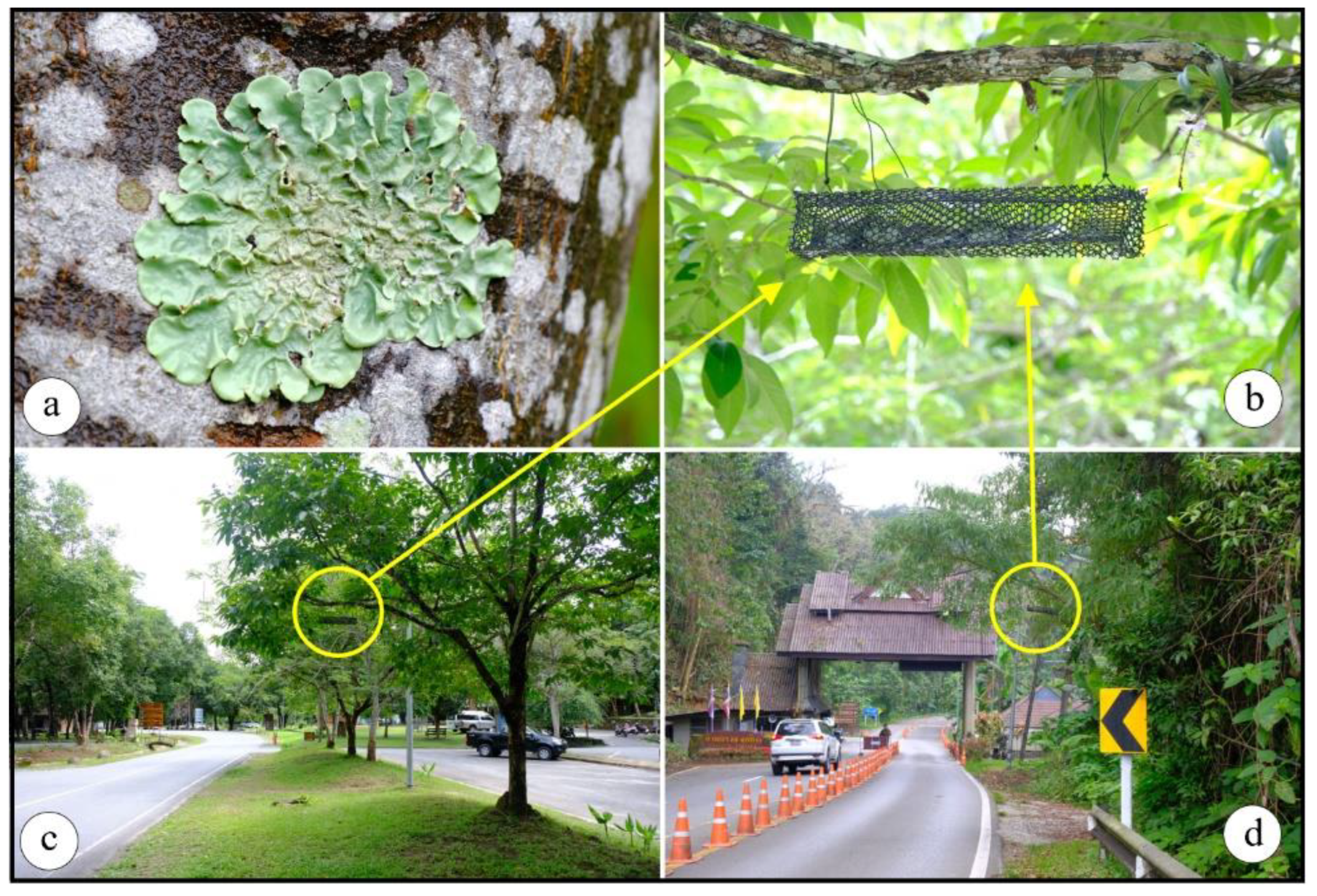
2.2. Lichen Preparation and Exposure

The epiphytic lichen P. tinctorum was selected as a biomonitoring tool for this study (Figure 3a). This lichen was chosen because (i) its population size is large enough for utilization, (ii) it is easy to identify and prepare, (iii) it has a high surface/mass (SM) ratio, which contributes to a higher capacity for element accumulation, and iv) its potential for bioaccumulation of air pollutants was demonstrated by several studies in Brazil [30,31,33], India [24], and Thailand [27,28,29]. Thalli of the lichen were collected on the bark of several host trees in the relatively unpolluted area in KYNP at elevations ranging from 700 to 800 m asl using stainless steel knives. All lichen thalli were checked for correct species identification and then cleaned by removing other lichen species, bark, debris, dirt, mosses, and insects. Approximately 10 cm2 of each thallus was fixed on an 8 × 8 cm polyethylene plastic netting (2 × 2 mm mesh size) using a fishing line. Subsequently, the samples were washed by submergence and shaking in deionized water. The washed samples were then placed in a nursery area for physiological adaptation and homogeneity for approximately 45 to 60 days before being exposed at the studied sites.
A total of 540 lichen thalli were used for the exposure in this study (15 thalli per site). For each exposure site and time, a lichen sample was picked up from the nursery and washed again by submergence and shaking in approximately 100 mL deionized water for approximately 2–3 min to clean and increase homogeneity in terms of initial element concentrations [34]. The washed samples were air-dried overnight. Five thalli were placed inside a 50 × 10 × 10 cm polyethylene cage (8 × 8 mm mesh size) at 15° to 30° inclination (Figure 3b). Three cages per site were hung on suitable tree branches or PVC pipes (if there were no suitable tree branches) (Figure 3b–d). The exposures were performed during the rainy and dry seasons for 90 days each. These seasons had different numbers of visitors, numbers of vehicles, and climatic conditions (Table 2). In the KYNP, the lichens were exposed from 16 June 2021 to 13 September 2021 (nursing during April 2021 to June 2021) during the rainy season and from 16 November 2021 to 13 February 2022 during the dry season (nursing during September 2021 to November 2021). At DINP, the lichens were exposed from 3 July 2021 to 30 September 2021 during the rainy season (nursing during April 2021 to June 2021) and from 23 November 2021 to 20 February 2022 during the dry season (nursing during September 2021 to November 2021).

2.3. Element Analysis

The lichen samples were dried and cleaned to remove debris and dirt from the lichen surfaces. The analysis of PTE concentrations in the lichen samples followed Sangiamdee (2014) [35] and Boonpeng et al. (2021) [34]. Briefly, the unwashed exposed lichen sample was immersed in liquid nitrogen and subsequently pulverized and homogenized with a ceramic mortar and pestle. It was then separated through a 500-μm sieve plate. Approximately 200 mg of the lichen powder was mineralized with 4 mL of concentrated HNO3 in a microwave digestion system (AIM 600, Aim Lab, Australia) at 140 °C for 40 min. The concentrations of 15 PTEs, including Al, As, Cd, Co, Cr, Cu, Fe, Mn, Mo, Ni, Pb, Sb, Ti, V, and Zn, were determined using inductively coupled plasma-mass spectrometry (ICP-MS, NexION 300Q, PerkinElmer, USA). The analytical quality was assessed with the certified reference material BCR-482 and spike samples. The recoveries (n = 7) ranged between 92.8% (V) and 101.8% (Fe). The analytical precision, expressed as percent relative standard deviation (%RSD), was less than 6% (n = 7) for all analyzed metals.

2.4. Data Analysis

The level of contamination of each PTE at each site was estimated using a contamination factor (CF): CF = Cm/Cc, where Cm is the average concentration of a PTE at a site, and Cc is the average concentration of the same PTE from a control site or an unpolluted site. At KYNP, the Cc of each PTE was obtained from the average concentration of the PTE during the rainy and dry seasons from the control site (KYC). At DINP, the Cc of each PTE was obtained from the average concentration of the PTE during the rainy and dry seasons from site DI1. This monitoring site was selected instead of DIC because (i) the lowest concentrations of most PTEs were found at DI1, (ii) the average CFs from all PTEs and seasons were lowest at DI1, and (iii) the average CFs from all PTEs and seasons were closest to the average CFs at the control site in the KYNP (KYC). The difference between the average CFs was only 0.08. The CF value was categorized into the following four classes: CF < 1.20 = no contamination, 1.20–2.00 = light contamination, 2.01–3.00 = medium contamination, and CF > 3 = heavy contamination. Subsequently, a pollution load index (PLI) was calculated using the CF: PLI = (CF1 × CF2 × CF3 ×…× CFn)1/n, where n is the number of studied PTEs. This index was originally used for estimating heavy metal pollution in estuarine ecosystems by Tomlinson et al. [36], and it has been frequently applied to several air pollution research to assess air pollution loads at monitoring sites [27,37,38,39,40,41]. The PLI value was categorized into the following five classes: PLI < 1.20 = no pollution, 1.20–1.50 = low pollution, 1.51–2.00 = moderate pollution, 2.01–2.50 = high pollution, and PLI > 2.50 = very high pollution [37].
The statistically significant difference among the PTE concentrations from each site, season, and park was tested using one-way analysis of variance (one-way ANOVA) and Tukey test for post hoc comparison at p < 0.05. All statistical analyses were performed using IBM SPSS Statistics 26 (IBM Corp, Armonk, NY, USA).

3. Results and Discussion

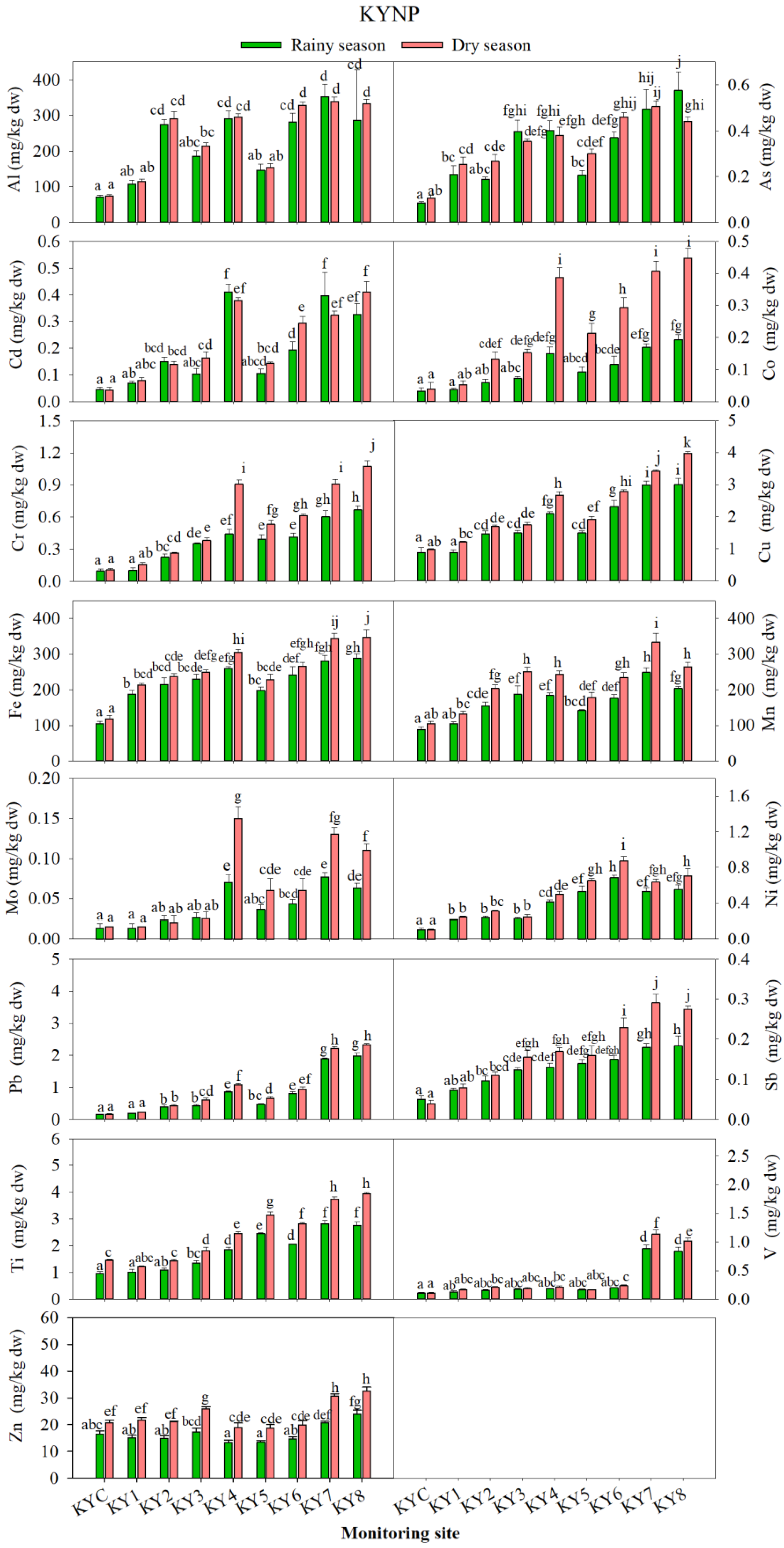
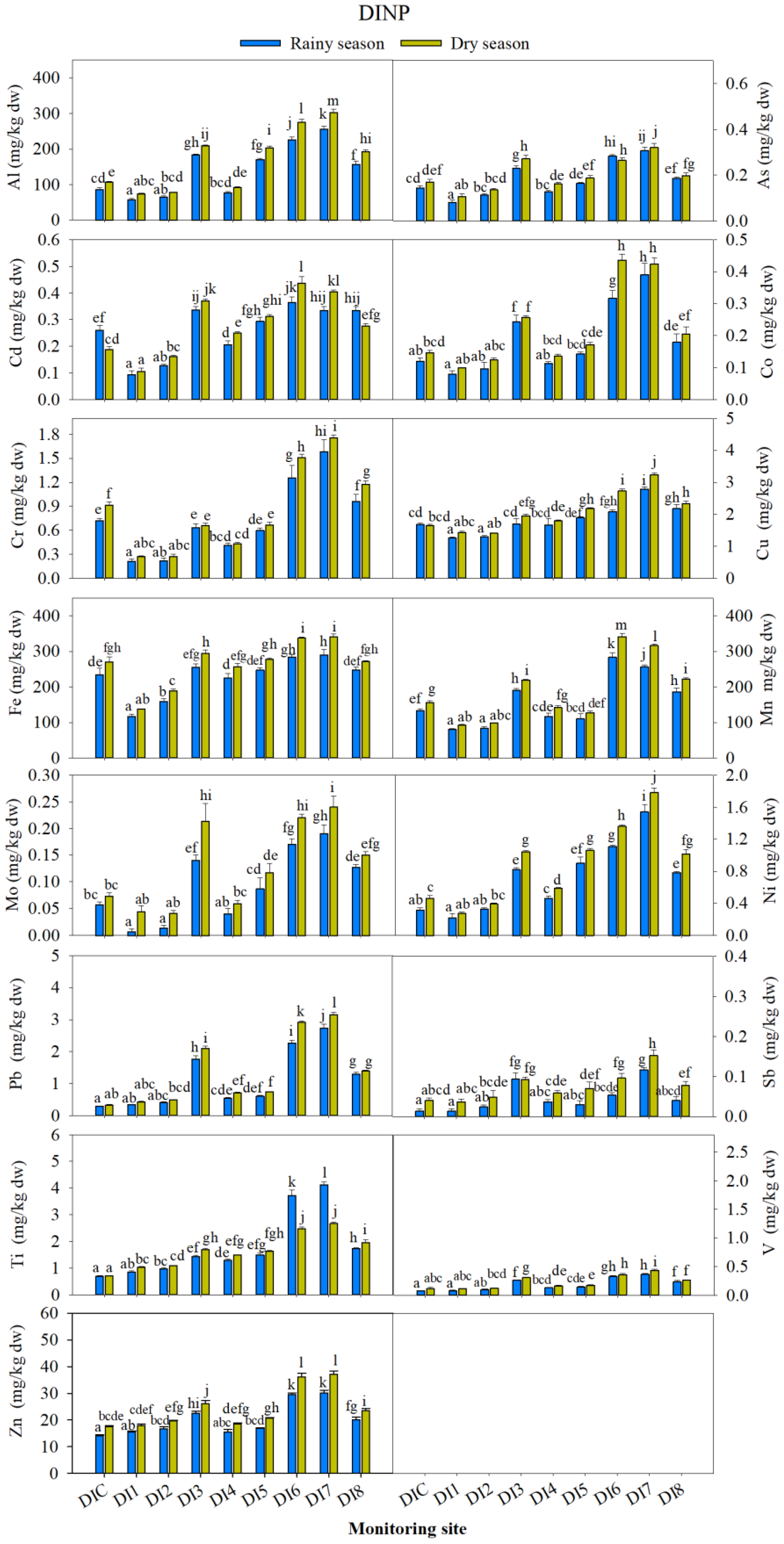
3.1. Concentrations of Potentially Toxic Elements in Lichens

At the KYNP, the concentrations of 13 out of 15 PTEs in the transplanted lichens P. tinctorum during the rainy and dry seasons were lowest at the control site (KYC) and were significantly lower (p < 0.05) than those at most monitoring sites. Only Zn and Ti showed the lowest concentrations at the other sites (Figure 4). The concentrations of all elements at most sites were higher or significantly higher (p < 0.05) during the dry season, which had lower rainfall amounts and higher numbers of visitors and motor vehicles. Apart from the KYC, most elements showed the lowest concentrations at the highest elevation site (KY1) and tended to be found at higher concentrations at the lower elevation sites, especially at the park entrance sites (KY7, KY8), which were located close to communities and had open areas with much less tree canopy.
At the DINP, the concentrations of 10 out of 15 PTEs during the rainy and dry seasons were lowest at DI1, which is the summit site at this park. In contrast, the highest concentrations of all PTEs were found at the monitoring sites located near the communities and park office (DI6, DI7, Figure 5). The atmosphere of the original assigned control site, DIC, did not show the lowest contamination caused by the investigated PTEs. The concentrations of 10 PTEs were higher or significantly higher (p < 0.05) than those at some monitoring sites, especially at DI1 and DI2. Only five PTEs, including Pb, Sb, Ti, V, and Zn showed the lowest concentrations at this site. This indicated that this location was not suitable for use as a control (unpolluted) site. However, the atmospheric contamination at this location probably originated from natural sources, i.e., rock and soil weathering, wind-blown dust, and the decomposition of dead materials, rather than anthropogenic sources from traffic vehicles or community activities. The concentrations of all elements at most sites were also higher or significantly higher (p < 0.05) during the dry season, which had lower rainfall amounts and higher numbers of visitors and motor vehicles.

3.2. Contamination Levels of Each Element in the Studied Sites

The contamination level of each PTE at each site was estimated using a CF value, which was based on the average concentration of each PTE found in the transplanted lichen P. tinctorum at the cleanest site of each park (KYC, DI1). At the KYNP, a total of 120 CFs from all PTEs at all monitoring sites (KY1–KY8) recorded during the rainy season were classified as showing no (14%), light (22%), medium (25%), and heavy (39%) contamination, while those recorded during the dry season were classified as showing no (6%), light (20%), medium (22%), and heavy (52%) contamination (Table 3). The PTE showing the highest contamination as indicated by the average CFs from all sites (excluding KYC) and seasons was Pb (6.19), followed by Cd (5.21), Co (5.15), Cr (4.96), Ni (4.58), Mo (4.07), As (3.79), Sb (3.54), V (3.46), Al (3.42), Cu (2.37), Fe (2.29), Mn (2.09), Ti (1.87), and Zn (1.08). All elements, except Zn, showed heavy contamination (CF > 3) at some sites, especially at the park entrances (KY7, KY8). At the DINP, the CFs from all monitoring sites recorded during the rainy season were categorized as showing no (24%), light (30%), medium (17%), and heavy (29%) contamination, while those recorded during the dry season were grouped as no (16%), light (27%), medium (26%), and heavy (31%) contamination. The PTE showing the highest contamination as indicated by the average CFs from all sites (excluding DIC) and seasons was Mo (4.58), followed by Pb (3.56), Ni (3.50), Cr (3.26), Cd (2.76), Sb (2.59), Al (2.49), Co (2.39), V (2.30), As (2.10), Mn (2.06), Ti (1.98), Fe (1.93), Cu (1.48), and Zn (1.37). All elements, except Cu, Fe, and Zn, showed heavy contamination at some sites, especially at sites close to the communities and park office (DI6, DI7). The range of the CF of each PTE from all monitoring sites in each park were illustrated in Table 4.
The PTEs in the air of the studied parks can originate from several sources. Tourism contribute PTEs through traffic vehicles and tourist activities such as cigarette smoking and camping [1,3,5,10,42]. Local anthropogenic sources include fossil fuel combustion by automobiles, agricultural activity, and open burning, while natural sources include rock and soil weathering, forest fire, wind-blown dust, and the decomposition of dead materials [6,13]. Irrespective of emission sources, these elements can be toxic to human health and organisms in ecosystems. Previous studies reported that the concentrations of some PTEs, including Co, Cu, Fe, Mn, Ni, Pb, and Zn, in the lichens Ramalina celastri and Usnea amblyoclada were correlated with pharyngitis, tonsilitis, asthma, laryngitis, and allergic rhinitis in children under six years old [43]. In addition, the concentration of Co in the lichen Canoparmelia texana was linked with cardiovascular diseases in adults [44]. The effects of each PTE on human health and plants were partly summarized in Table 5.

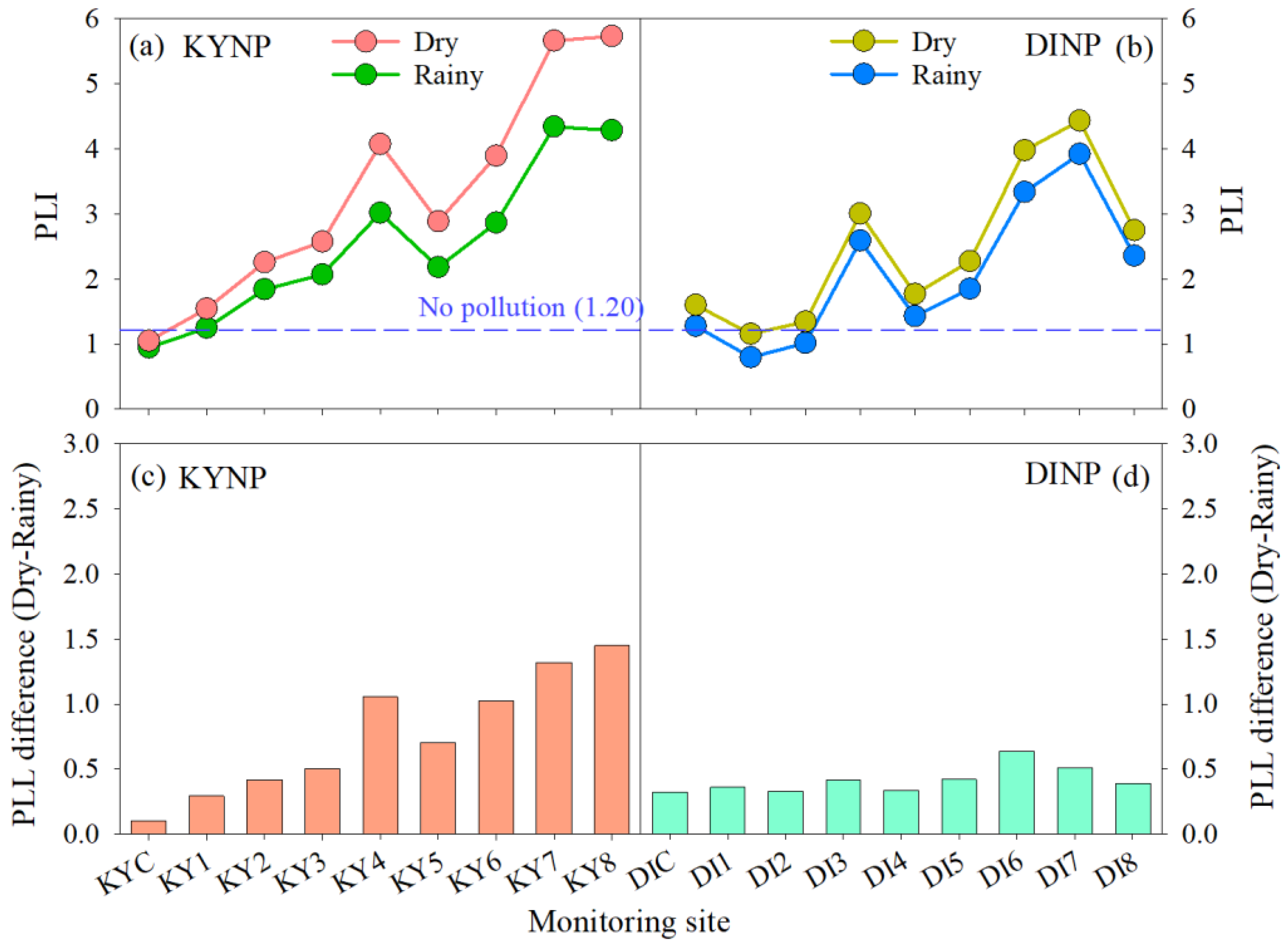
3.3. Air Pollution Level at Each Monitoring Site

The level of air pollution based on the 15 investigated PTEs at each site, season, and park was revealed by the PLI. This index is frequently used to estimate air pollution loads at the studied sites in previous studies [27,38,39,40,41,78]. At the KYNP, the PLIs at all sites during the dry season were higher than those during the rainy season (Figure 6a), which indicated higher pollution loads during the dry season. During the dry season, the lowest PLI (1.05) was observed at the control site (KYC) and was classified as no pollution, while the PLIs at eight monitoring sites ranged from 1.55 to 5.73 (mean of 3.58) and were classified as medium to very high pollution. During the rainy season, the PLI was also lowest at the control site (0.95) and was grouped as no pollution, whereas the PLIs at the other sites ranged from 1.25 to 4.34 (mean of 2.73) and were categorized as light to very high pollution (Table 3). The slightly higher PLI at the KYC during the dry season compared to the rainy season probably came from natural origins such as rock and soil weathering, wind-blown dust, and the decomposition of dead materials. In addition, rainfall and air humidity were also the main factors that determined the concentrations of air pollutants. Rainfall can remove pollutants from the air, and air humidity can reduce the resuspension of soil dust and the diffusion of air pollutants. The different gaps in the PLIs between the rainy and dry seasons at the monitoring sites (Figure 6c) probably originated from natural origins, road traffic, and tourist activities. The numbers of visitors and vehicles during the dry season were approximately 2.7 and 2.1 times higher at the KYNP and DINP (Table 2), respectively, than those during the rainy season. Automobiles release elemental pollutants into the air via fossil fuel combustion, brake abrasives, clutch systems, tire wear, engines and components, road damage, and the resuspension of soil dust [22,79,80]. In addition, tourist activities such as cigarette smoking and camping might contribute some pollutants to the air [10]. Excluding the KYC, the lowest PLI was observed at the summit site (KY1), and it then increased at the lower elevation sites and was highest at the park entrances (KY7, KY8). These two sites were located closer to communities, urban areas, and roads, and had higher number of automobiles. The average PLIs of all sites in both seasons in descending order were as follows: KY8 > KY7 > KY4 > KY6 > KY5 > KY3 > KY2 > KY1 > KYC. The PLIs of four sites, KY4, KY6, KY7, and KY8, were estimated as having very high pollution during both seasons, while KY3 and KY5 showed very high pollution during the dry season. The category of no pollution was not found from all eight monitoring sites, and the light pollution category was only observed at the summit site, KY1, and during the rainy season.
The PLIs at all sites in the DINP were also higher during the dry season than during the rainy season (Figure 6b). The numbers of visitors and vehicles were higher during the dry season (Table 2). During the dry season, the lowest PLI was found at the summit site, DI1 (1.16), and was grouped as no pollution. The PLIs at all monitoring sites (including DI1) ranged from 1.16 to 4.43 (mean of 2.59) and were classified as having no to very high pollution. During the rainy season, the PLI was lowest at the DI1 (0.80) as well and was classified as no pollution. Meanwhile, the PLIs at all monitoring site ranged from 0.80 to 3.92 (mean of 2.16) and showed no to very high pollution. Unexpectedly, the PLIs at the original assigned control site (DIC) were the third lowest in both seasons, after DI1 and DI2. Because this site was located inside the forest with dense canopy and approximately 600 m far from the main road, the contamination of the PTEs at this site probably originated from the natural source as mentioned earlier. The average CFs of all PTEs and seasons at the DI1 were close to those at the KYC (the control site at KYNP). Therefore, the baseline of atmospheric contamination caused by the investigated PTEs in this park was considered at the DI1 instead. The higher PLI recorded at the DIC during the dry season than during the rainy season probably came from natural origins, as occurred in the KYNP. The higher different gaps in the PLIs at DI6 and DI7 compared to the other sites indicated more impacts from road traffic and human activities (Figure 6d). These sites were located close to the local communities, local market, and park office, and they had a higher traffic density. The average PLIs of all sites in both seasons in descending order were as follows: DI7 > DI6 > DI3 > DI8 > DI5 > DI4 > DIC > DI2 > DI1. The PLIs of three sites, DI3, DI6 and DI7, were estimated as having very high pollution in both seasons, and DI8 showed very high pollution during the dry season. The category of no pollution was observed at DI1 and DI2, and the light pollution could be found at DIC, DI2 and DI4.
The higher atmospheric contamination caused by the investigated PTEs during the dry season were clearly demonstrated in both mountains. This season obviously had the higher number of visitors and vehicles; thus, this contamination may have come from road traffic and tourist activities. Moreover, locations that had higher traffic vehicles and tourist’s activities also showed higher pollution loads as indicated by the PLIs. This finding can indicate the impact of tourism on atmospheric contamination in natural areas. The monitoring sites were designed to locate the roadside from the park entrances to the summit points; therefore, the obtained data can reveal the atmospheric contamination in the ecosystems and communities along the roads. Forest ecosystems were located alongside the roads, and most of the monitoring sites were located at forest edges; thus, this result can indicate forest edge contamination. Several organisms, such as flowering plants, bryophytes, ferns, lichens, fungi, and animals, were found at these forest edges. Air pollution can destroy them, especially the sensitive groups, such as lichens and bryophytes. In addition, the air quality of the nearby communities was also affected. Overall, the result of this study can be used for planning and managing tourism in parks for the sustainability of natural areas and for protecting human health.
This study was performed during the COVID-19 pandemic in Thailand, which restricted the numbers of visitors and vehicles in parks. At the KYNP, the numbers of visitors and vehicles were approximately 35% and 16% lower during the rainy season and 10% and 6% lower during the dry season, respectively, than those in 2019 before the COVID-19 pandemic in Thailand. Moreover, at the DINP, the numbers of visitors and vehicles were approximately 99.9% and 100% lower during the rainy season and 48% and 37% lower during the dry season, respectively, than those in 2019. The pollution level might be different when tourism is in full swing; thus, reinvestigation is needed to reveal the air pollution situation during the time of normal tourism activity in parks. This study confirms that the air of the mountain areas can be contaminated by PTEs of both natural and anthropogenic origins. Thus, the appropriate planning and management of tourism and human activities in naturally revered areas will promote good health and sustainable ecosystems. There are several pollutants emitted from automobiles, such as NO2, SO2, PAHs, VOCs, and other PTEs, and measuring these pollutants will reveal the overall air quality in parks. The extent of air pollutant diffusion and monitoring inside forests should be investigated to estimate forest contamination. Lastly, air quality can change with space and time, and regular measurements are necessary for a sustainable environment in natural areas.

4. Conclusions

Levels of air pollution based on the 15 investigated PTEs during the rainy and dry seasons at the KYNP and DINP could be assessed by the transplanted lichen P. tinctorum. The result clearly illustrated that the atmosphere of several monitoring sites in the mountain areas was contaminated by the investigated PTEs. Based on the concentrations of PTEs found at the KYC and DI1, PLIs at many sites in the KYNP and DINP were categorized as having very high pollution. The lowest air pollution loads were observed at the summit site in each park. Higher air pollution loads were found at sites close to higher traffic density and communities, including the park entrances at the KYNP and the community sites at the DINP. The higher pollution loads were observed during the dry season in both mountains. This pollution probably came from road traffic, tourist’s activities (cigarette smoking, camping), and agricultural practice. The drier season was also another factor determining the concentrations of airborne PTEs, as it contributes to the resuspension of soil dust and the diffusion of air pollutants. The CFs revealed that several PTEs heavily contaminated many sites in both mountains. The results of this study indicate that tourism and communities can pollute the air in natural areas. This study can be useful for park management to help maintain good health and ecosystem sustainability. Reinvestigation and studies on different kinds of air pollutants are needed to achieve overall good air quality within parks.

Author Contributions

Conceptualization, C.B.; Methodology, C.B., D.S. and S.N.; Formal analysis, C.B.; Investigation, C.B. and S.N.; Writing—Original Draft Preparation, C.B.; Writing—Review and Editing, C.B. and K.B.; Supervision, K.B.; Project Administration, C.B.; Funding Acquisition, C.B. All authors have read and agreed to the published version of the manuscript.

Funding

This research was funded by the Thailand Science Research and Innovation (TSRI) and the APC was funded by Ramkhamhaeng University.

Institutional Review Board Statement

Not applicable.

Informed Consent Statement

Not applicable.

Data Availability Statement

All data generated or analyzed during this study are included in this published article, and the raw data are available from the corresponding author upon reasonable request.

Acknowledgments

We thank Marisa Pischom, Pawanrat Butrid, Pitakchai Fuangkeaw, and Mongkol Phaengphech for helping with fieldwork and laboratory measurements. Many thanks also go to the staff of the Khao Yai National Park, the Doi Inthanon National Park, and the Inthanon Paphiopedilum orchid conservation project for supporting the fieldwork. We also appreciate the anonymous reviewers for providing valuable comments and suggestions. This work was financially supported by the Thailand Science Research and Innovation (TSRI).

Conflicts of Interest

The authors declare no conflict of interest.

References

  1. Guidotti, M.; Stella, D.; Dominici, C.; Blasi, G.; Owczarek, M.; Vitali, M.; Protano, C. Monitoring of traffic-related pollution in a province of central Italy with transplanted lichen Pseudevernia furfuracea. Bull. Environ. Contam. Toxicol. 2009, 83, 852–858. [Google Scholar] [CrossRef]
  2. Nascimbene, J.; Tretiach, M.; Corana, F.; Lo Schiavo, F.; Kodnik, D.; Dainese, M.; Mannucci, B. Patterns of traffic polycyclic aromatic hydrocarbon pollution in mountain areas can be revealed by lichen biomonitoring: A case study in the Dolomites (Eastern Italian Alps). Sci. Total Environ. 2014, 475, 90–96. [Google Scholar] [CrossRef] [PubMed]
  3. Yemets, O.A.; Solhaug, K.A.; Gauslaa, Y. Spatial dispersal of airborne pollutants and their effects on growth and viability of lichen transplants along a rural highway in Norway. Lichenol. 2014, 46, 809–823. [Google Scholar] [CrossRef]
  4. Osborne, S.; Uche, O.; Mitsakou, C.; Exley, K.; Dimitroulopoulou, S. Air quality around schools: Part I—A comprehensive literature review across high-income countries. Environ. Res. 2021, 196, 110817. [Google Scholar] [CrossRef]
  5. Zhao, L.; Zhang, C.; Jia, S.; Liu, Q.; Chen, Q.; Li, X.; Liu, X.; Wu, Q.; Zhao, L.; Liu, H. Element bioaccumulation in lichens transplanted along two roads: The source and integration time of elements. Ecol. Indic. 2019, 99, 101–107. [Google Scholar] [CrossRef]
  6. Vannini, A.; Tedesco, R.; Loppi, S.; Di Cecco, V.; Di Martino, L.; Nascimbene, J.; Dallo, F.; Barbante, C. Lichens as monitors of the atmospheric deposition of potentially toxic elements in high elevation Mediterranean ecosystems. Sci. Total Environ. 2021, 798, 149369. [Google Scholar] [CrossRef]
  7. Chahloul, N.; Khadhri, A.; Vannini, A.; Mendili, M.; Raies, A.; Loppi, S. Bioaccumulation of potentially toxic elements in some lichen species from two remote sites of Tunisia. Biologia 2022, 77, 2469–2473. [Google Scholar] [CrossRef]
  8. Khodadadi, R.; Sohrabi, M.; Loppi, S.; Birgani, Y.T.; Babaei, A.A.; Neisi, A.; Baboli, Z.; Dastoorpoor, M.; Goudarzi, G. Atmospheric pollution by potentially toxic elements: Measurement and risk assessment using lichen transplants. Int. J. Environ. Health Res. 2023, 1–14. [Google Scholar] [CrossRef]
  9. Klapstein, S.J.; Walker, A.K.; Saunders, C.H.; Cameron, R.P.; Murimboh, J.D.; O’Driscoll, N.J. Spatial distribution of mercury and other potentially toxic elements using epiphytic lichens in Nova Scotia. Chemosphere 2020, 241, 125064. [Google Scholar] [CrossRef] [PubMed]
  10. Paoli, L.; Maccelli, C.; Guarnieri, M.; Vannini, A.; Loppi, S. Lichens “travelling” in smokers’ cars are suitable biomonitors of indoor air quality. Ecol. Indic. 2019, 103, 576–580. [Google Scholar] [CrossRef]
  11. Incerti, G.; Cecconi, E.; Capozzi, F.; Adamo, P.; Bargagli, R.; Benesperi, R.; Carniel, F.C.; Cristofolini, F.; Giordano, S.; Puntillo, D.; et al. Infraspecific variability in baseline element composition of the epiphytic lichen Pseudevernia furfuracea in remote areas: Implications for biomonitoring of air pollution. Environ. Sci. Pollut. Res. 2017, 24, 8004–8016. [Google Scholar] [CrossRef]
  12. Loppi, S. Lichens as sentinels for air pollution at remote alpine areas (Italy). Environ. Sci. Pollut. Res. 2014, 21, 2563–2571. [Google Scholar] [CrossRef]
  13. Liu, H.-J.; Zhao, L.-C.; Fang, S.-B.; Liu, S.-W.; Hu, J.-S.; Wang, L.; Liu, X.-D.; Wu, Q.-F. Use of the lichen Xanthoria mandschurica in monitoring atmospheric elemental deposition in the Taihang Mountains, Hebei, China. Sci. Rep. 2016, 6, 23456. [Google Scholar] [CrossRef] [Green Version]
  14. Achotegui-Castells, A.; Sardans, J.; Ribas, À.; Peñuelas, J. Identifying the origin of atmospheric inputs of trace elements in the Prades Mountains (Catalonia) with bryophytes, lichens, and soil monitoring. Environ. Monit. Assess. 2013, 185, 615–629. [Google Scholar] [CrossRef]
  15. Klimek, B.; Tarasek, A.; Hajduk, J. Trace element concentrations in lichens xollected in the Beskidy mountains, the outer western Carpathians. Bull. Environ. Contam. Toxicol. 2015, 94, 532–536. [Google Scholar] [CrossRef] [Green Version]
  16. McMurray, J.A.; Roberts, D.W.; Geiser, L.H. Epiphytic lichen indication of nitrogen deposition and climate in the northern rocky mountains, USA. Ecol. Indic. 2015, 49, 154–161. [Google Scholar] [CrossRef]
  17. Root, H.T.; Geiser, L.H.; Jovan, S.; Neitlich, P. Epiphytic macrolichen indication of air quality and climate in interior forested mountains of the Pacific Northwest, USA. Ecol. Indic. 2015, 53, 95–105. [Google Scholar] [CrossRef]
  18. Nash, T.H., III. Lichen Biology, 2nd ed.; Cambridge University Press: New York, NY, USA, 2008; p. 486. [Google Scholar]
  19. Bargagli, R.; Mikhailova, I. Accumulation of inorganic contaminations. In Monitoring with Lichens—Monitoring Lichens; Nimis, P.L., Scheidegger, C., Wolseley, P.A., Eds.; Kluwer Academic: Dordrecht, The Netherlands, 2002; pp. 65–84. [Google Scholar]
  20. Garty, J. Biomonitoring atmospheric heavy metals with lichens: Theory and application. Crit. Rev. Plant Sci. 2001, 20, 309–371. [Google Scholar] [CrossRef]
  21. Cecconi, E.; Fortuna, L.; Peplis, M.; Tretiach, M. Element accumulation performance of living and dead lichens in a large-scale transplant application. Environ. Sci. Pollut. Res. 2021, 28, 16214–16226. [Google Scholar] [CrossRef] [PubMed]
  22. Winkler, A.; Contardo, T.; Lapenta, V.; Sgamellotti, A.; Loppi, S. Assessing the impact of vehicular particulate matter on cultural heritage by magnetic biomonitoring at Villa Farnesina in Rome, Italy. Sci. Total Environ. 2022, 823, 153729. [Google Scholar] [CrossRef] [PubMed]
  23. Brunialti, G.; Frati, L. Bioaccumulation with lichens: The Italian experience. Int. J. Environ. Stud. 2014, 71, 15–26. [Google Scholar] [CrossRef]
  24. Daimari, R.; Bhuyan, P.; Hussain, S.; Nayaka, S.; Mazumder, M.A.J.; Hoque, R.R. Anatomical, physiological, and chemical alterations in lichen (Parmotrema tinctorum (Nyl.) Hale) transplants due to air pollution in two cities of Brahmaputra Valley, India. Environ. Monit. Assess. 2021, 193, 101. [Google Scholar] [CrossRef]
  25. Paoli, L.; Fačkovcová, Z.; Guttová, A.; Maccelli, C.; Kresáňová, K.; Loppi, S. Evernia goes to school: Bioaccumulation of heavy metals and photosynthetic performance in lichen transplants exposed indoors and uutdoors in public and private environments. Plants 2019, 8, 125. [Google Scholar] [CrossRef] [Green Version]
  26. Massimi, L.; Conti, M.E.; Mele, G.; Ristorini, M.; Astolfi, M.L.; Canepari, S. Lichen transplants as indicators of atmospheric element concentrations: A high spatial resolution comparison with PM10 samples in a polluted area (Central Italy). Ecol. Indic. 2019, 101, 759–769. [Google Scholar] [CrossRef]
  27. Boonpeng, C.; Polyiam, W.; Sriviboon, C.; Sangiamdee, D.; Watthana, S.; Nimis, P.L.; Boonpragob, K. Airborne trace elements near a petrochemical industrial complex in Thailand assessed by the lichen Parmotrema tinctorum (Despr. ex Nyl.) Hale. Environ. Sci. Pollut. Res. 2017, 24, 12393–12404. [Google Scholar] [CrossRef] [PubMed]
  28. Boonpeng, C.; Sangiamdee, D.; Noikrad, S.; Watthana, S.; Boonpragob, K. Metal accumulation in lichens as a tool for assessing atmospheric contamination in a natural park. Environ. Nat. Resour. J. 2020, 18, 166–176. [Google Scholar] [CrossRef]
  29. Boonpeng, C.; Sriviboon, C.; Polyiam, W.; Sangiamdee, D.; Watthana, S.; Boonpragob, K. Assessing atmospheric pollution in a petrochemical industrial district using a lichen-air quality index (LiAQI). Ecol. Indic. 2018, 95, 589–594. [Google Scholar] [CrossRef]
  30. Palharini, K.M.Z.; Vitorino, L.C.; Bessa, L.A.; de Carvalho Vasconcelos Filho, S.; Silva, F.G. Parmotrema tinctorum as an indicator of edge effect and air quality in forested areas bordered by intensive agriculture. Environ. Sci. Pollut. Res. 2021, 28, 68997–69011. [Google Scholar] [CrossRef] [PubMed]
  31. Port, R.K.; Käffer, M.I.; Schmitt, J.L. Morphophysiological variation and metal concentration in the thallus of Parmotrema tinctorum (Despr. ex Nyl.) Hale between urban and forest areas in the subtropical region of Brazil. Environ. Sci. Pollut. Res. 2018, 25, 33667–33677. [Google Scholar] [CrossRef]
  32. Zulaini, A.A.M.; Muhammad, N.; Asman, S.; Hashim, N.H.; Jusoh, S.; Abas, A.; Yusof, H.; Din, L. Evaluation of transplanted lichens, Parmotrema tinctorum and Usnea diffracta as bioindicator on heavy metals accumulation in southern peninsular Malaysia. J. Sustain. Sci. Manag. 2019, 14, 1–13. [Google Scholar]
  33. Koch, N.M.; Branquinho, C.; Matos, P.; Pinho, P.; Lucheta, F.; Martins, S.M.A.; Vargas, V.M.F. The application of lichens as ecological surrogates of air pollution in the subtropics: A case study in South Brazil. Environ. Sci. Pollut. Res. 2016, 23, 20819–20834. [Google Scholar] [CrossRef]
  34. Boonpeng, C.; Sangiamdee, D.; Noikrad, S.; Boonpragob, K. Influence of washing thalli on element concentrations of the epiphytic and epilithic lichen Parmotrema tinctorum in the tropic. Environ. Sci. Pollut. Res. 2021, 28, 9723–9730. [Google Scholar] [CrossRef] [PubMed]
  35. Sangiamdee, D. Validation of Sample Preparation Methods for Determination of Metal Accumulation in Lichen Parmotrema tinctorum by Inductively Coupled Plasma Mass Spectrometry (ICP-MS). Master’s Thesis, Ramkhamhaeng University, Bangkok, Thailand, 2014. [Google Scholar]
  36. Tomlinson, D.L.; Wilson, J.G.; Harris, C.R.; Jeffrey, D.W. Problems in the assessment of heavy-metal levels in estuaries and the formation of a pollution index. Helgol. Mar. Res. 1980, 33, 566–575. [Google Scholar] [CrossRef] [Green Version]
  37. Boonpeng, C.; Sangiamdee, D.; Noikrad, S.; Boonpragob, K. Lichen biomonitoring of seasonal outdoor air quality at schools in an industrial city in Thailand. Environ. Sci. Pollut. Res. 2023. [Google Scholar]
  38. Boamponsem, L.K.; Adam, J.I.; Dampare, S.B.; Nyarko, B.J.B.; Essumang, D.K. Assessment of atmospheric heavy metal deposition in the Tarkwa gold mining area of Ghana using epiphytic lichens. Nucl. Instrum. Methods Phys. Res. Sect. B Beam Interact. Mater. At. 2010, 268, 1492–1501. [Google Scholar] [CrossRef]
  39. Salo, H.; Bućko, M.S.; Vaahtovuo, E.; Limo, J.; Mäkinen, J.; Pesonen, L.J. Biomonitoring of air pollution in SW Finland by magnetic and chemical measurements of moss bags and lichens. J. Geochem. Explor. 2012, 115, 69–81. [Google Scholar] [CrossRef]
  40. Sergeeva, A.; Zinicovscaia, I.; Vergel, K.; Yushin, N.; Urošević, M.A. The effect of heavy industry on air pollution studied by active moss biomonitoring in Donetsk region (Ukraine). Arch. Environ. Contam. Toxicol. 2021, 80, 546–557. [Google Scholar] [CrossRef] [PubMed]
  41. Saib, H.; Yekkour, A.; Toumi, M.; Guedioura, B.; Benamar, M.A.; Zeghdaoui, A.; Austruy, A.; Bergé-Lefranc, D.; Culcasi, M.; Pietri, S. Lichen biomonitoring of airborne trace elements in the industrial-urbanized area of eastern algiers (Algeria). Atmos. Pollut. Res. 2022, 14, 101643. [Google Scholar] [CrossRef]
  42. González, C.M.; Casanovas, S.S.; Pignata, M.L. Biomonitoring of air pollutants from traffic and industries employing Ramalina ecklonii (Spreng.) Mey. and Flot. in Córdoba, Argentina. Environ. Pollut. 1996, 91, 269–277. [Google Scholar] [CrossRef]
  43. Carreras, H.A.; Wannaz, E.D.; Pignata, M.L. Assessment of human health risk related to metals by the use of biomonitors in the province of Córdoba, Argentina. Environ. Pollut. 2009, 157, 117–122. [Google Scholar] [CrossRef]
  44. Saiki, M.; Santos, J.O.; Alves, E.R.; Genezini, F.A.; Marcelli, M.P.; Saldiva, P.H.N. Correlation study of air pollution and cardio-respiratory diseases through NAA of an atmospheric pollutant biomonitor. J. Radioanal. Nucl. Chem. 2014, 299, 773–779. [Google Scholar] [CrossRef]
  45. ATSDR. The ATSDR 2022 Substance Priority List. Available online: https://www.atsdr.cdc.gov/spl/index.html#2019spl (accessed on 14 February 2023).
  46. IARC. IARC Monographs on the Identification of Carcinogenic Hazards to Humans. Available online: https://monographs.iarc.who.int/list-of-classifications (accessed on 2 November 2022).
  47. ATSDR. Aluminum. Available online: https://wwwn.cdc.gov/TSP/substances/ToxSubstance.aspx?toxid=34 (accessed on 16 February 2023).
  48. Panda, S.K.; Baluska, F.; Matsumoto, H. Aluminum stress signaling in plants. Plant Signal Behav. 2009, 4, 592–597. [Google Scholar] [CrossRef] [Green Version]
  49. ATSDR. Arsenic. Available online: https://wwwn.cdc.gov/TSP/substances/ToxSubstance.aspx?toxid=3 (accessed on 2 November 2022).
  50. Finnegan, P.M.; Chen, W. Arsenic toxicity: The effects on plant metabolism. Front. Physiol. 2012, 3, 182. [Google Scholar] [CrossRef] [Green Version]
  51. ATSDR. Cadmium. Available online: https://wwwn.cdc.gov/TSP/substances/ToxSubstance.aspx?toxid=15 (accessed on 2 November 2022).
  52. Haider, F.U.; Liqun, C.; Coulter, J.A.; Cheema, S.A.; Wu, J.; Zhang, R.; Wenjun, M.; Farooq, M. Cadmium toxicity in plants: Impacts and remediation strategies. Ecotoxicol. Environ. Saf. 2021, 211, 111887. [Google Scholar] [CrossRef] [PubMed]
  53. ATSDR. Cobalt. Available online: https://wwwn.cdc.gov/TSP/substances/ToxSubstance.aspx?toxid=64 (accessed on 2 November 2022).
  54. Mahey, S.; Kumar, R.; Sharma, M.; Kumar, V.; Bhardwaj, R. A critical review on toxicity of cobalt and its bioremediation strategies. SN Appl. Sci. 2020, 2, 1279. [Google Scholar] [CrossRef]
  55. ATSDR. Chromium. Available online: https://wwwn.cdc.gov/TSP/substances/ToxSubstance.aspx?toxid=17 (accessed on 2 November 2022).
  56. Prasad, S.; Yadav, K.K.; Kumar, S.; Gupta, N.; Cabral-Pinto, M.M.S.; Rezania, S.; Radwan, N.; Alam, J. Chromium contamination and effect on environmental health and its remediation: A sustainable approaches. J. Environ. Manag. 2021, 285, 112174. [Google Scholar] [CrossRef] [PubMed]
  57. ATSDR. Copper. Available online: https://wwwn.cdc.gov/TSP/substances/ToxSubstance.aspx?toxid=37 (accessed on 2 November 2022).
  58. Mir, A.R.; Pichtel, J.; Hayat, S. Copper: Uptake, toxicity and tolerance in plants and management of Cu-contaminated soil. Biometals 2021, 34, 737–759. [Google Scholar] [CrossRef]
  59. Porter, J.L.; Rawla, P. Hemochromatosis. Available online: https://www.ncbi.nlm.nih.gov/books/NBK430862/ (accessed on 16 February 2023).
  60. Connolly, E.L.; Guerinot, M. Iron stress in plants. Genome Biol. 2002, 3, 1–4. [Google Scholar] [CrossRef] [Green Version]
  61. ATSDR. Manganese. Available online: https://wwwn.cdc.gov/TSP/substances/ToxSubstance.aspx?toxid=23 (accessed on 18 December 2022).
  62. Fernando, D.R.; Lynch, J.P. Manganese phytotoxicity: New light on an old problem. Ann. Bot. 2015, 116, 313–319. [Google Scholar] [CrossRef]
  63. ATSDR. Molybdenum. Available online: https://wwwn.cdc.gov/TSP/substances/ToxSubstance.aspx?toxid=289 (accessed on 2 November 2022).
  64. Xu, S.; Hu, C.; Tan, Q.; Qin, S.; Sun, X. Subcellular distribution of molybdenum, ultrastructural and antioxidative responses in soybean seedlings under excess molybdenum stress. Plant Physiol. Biochem. 2018, 123, 75–80. [Google Scholar] [CrossRef]
  65. ATSDR. Nickel. Available online: https://wwwn.cdc.gov/TSP/substances/ToxSubstance.aspx?toxid=44 (accessed on 16 February 2023).
  66. Hassan, M.U.; Chattha, M.U.; Khan, I.; Chattha, M.B.; Aamer, M.; Nawaz, M.; Ali, A.; Khan, M.A.U.; Khan, T.A. Nickel toxicity in plants: Reasons, toxic effects, tolerance mechanisms, and remediation possibilities—A review. Environ. Sci. Pollut. Res. 2019, 26, 12673–12688. [Google Scholar] [CrossRef]
  67. ATSDR. Lead. Available online: https://wwwn.cdc.gov/TSP/substances/ToxSubstance.aspx?toxid=22 (accessed on 2 November 2022).
  68. EPA. Lead Air Pollution; United States Environmental Protection Agency (EPA): Washington, DC, USA, 2022.
  69. Pourrut, B.; Shahid, M.; Dumat, C.; Winterton, P.; Pinelli, E. Lead uptake, toxicity, and detoxification in plants. Rev. Environ. Contam. Toxicol. 2011, 213, 113–136. [Google Scholar] [CrossRef] [Green Version]
  70. ATSDR. Antimony. Available online: https://wwwn.cdc.gov/TSP/substances/ToxSubstance.aspx?toxid=58 (accessed on 2 November 2022).
  71. Feng, R.; Wei, C.; Tu, S.; Ding, Y.; Wang, R.; Guo, J. The uptake and detoxification of antimony by plants: A review. Environ. Exp. Bot. 2013, 96, 28–34. [Google Scholar] [CrossRef]
  72. ATSDR. Titanium Tetrachloride. Available online: https://wwwn.cdc.gov/TSP/substances/ToxSubstance.aspx?toxid=122 (accessed on 2 November 2022).
  73. Cox, A.; Venkatachalam, P.; Sahi, S.; Sharma, N. Silver and titanium dioxide nanoparticle toxicity in plants: A review of current research. Plant Physiol. Biochem. 2016, 107, 147–163. [Google Scholar] [CrossRef]
  74. ATSDR. Vanadium. Available online: https://wwwn.cdc.gov/TSP/substances/ToxSubstance.aspx?toxid=50 (accessed on 2 November 2022).
  75. Altaf, M.A.; Shu, H.; Hao, Y.; Zhou, Y.; Mumtaz, M.A.; Wang, Z. Vanadium Toxicity Induced Changes in Growth, Antioxidant Profiling, and Vanadium Uptake in Pepper (Capsicum annum L.) Seedlings. Horticulturae 2022, 8, 28. [Google Scholar] [CrossRef]
  76. ATSDR. Zinc. Available online: https://wwwn.cdc.gov/TSP/substances/ToxSubstance.aspx?toxid=54 (accessed on 16 February 2023).
  77. Kaur, H.; Garg, N. Zinc toxicity in plants: A review. Planta 2021, 253, 129. [Google Scholar] [CrossRef]
  78. Paoli, L.; Guttová, A.; Grassi, A.; Lackovičová, A.; Senko, D.; Sorbo, S.; Basile, A.; Loppi, S. Ecophysiological and ultrastructural effects of dust pollution in lichens exposed around a cement plant (SW Slovakia). Environ. Sci. Pollut. Res. 2015, 22, 15891–15902. [Google Scholar] [CrossRef]
  79. Rienda, I.C.; Alves, C.A. Road dust resuspension: A review. Atmos. Res. 2021, 261, 105740. [Google Scholar] [CrossRef]
  80. Spellerberg, I.F. Ecological effects of roads and traffic: A literature review. Glob. Ecol. Biogeogr. Lett. 1998, 7, 317–333. [Google Scholar] [CrossRef]
Figure 1. Locations of control (KYC, DIC) and monitoring (KY1–KY8, DI1–DI8) sites in Khao Yai National Park (KYNP) and Doi Inthanon National Park (DINP) in Thailand.
Forests 14 00611 g001
Figure 2. Yearly numbers of visitors (a) and vehicles (b) from 2013 to 2021 and monthly numbers of visitors (c) and vehicles (d) averaged from 2016 to 2019 (Source: National Parks of Thailand; Available online: https://portal.dnp.go.th/Content/nationalpark?contentId=22377 (accessed on 14 February 2023)).
Forests 14 00611 g002
Figure 3. Thallus of the lichen Parmotrema tinctorum (a), lichen samples exposed at a monitoring site (b), the environment at site KY3 in Khao Yai National Park (c) and at site DI3 in Doi Inthanon National Park (d).
Forests 14 00611 g003
Figure 4. Average concentration of each potentially toxic element (PTE, n = 3) at each site during the rainy and dry seasons in Khao Yai National Park (KYNP). The different letters on a graph of each PTE indicates statistically significant difference by one-way ANOVA with Tukey test, p < 0.05, n = 3.
Forests 14 00611 g004
Figure 5. Average concentration of each potentially toxic element (PTE, n = 3) at each site during the rainy and dry seasons in Doi Inthanon National Park (DINP). The different letters on a graph of each PTE indicates statistically significant difference by one-way ANOVA with Tukey test, p < 0.05, n = 3.
Forests 14 00611 g005
Figure 6. Pollution load index (PLI) at each site during the rainy and dry seasons in Khao Yai National Park (KYNP, a) and Doi Inthanon National Park (DINP, b). Difference between the PLI during the rainy and dry seasons at each site in the KYNP (c) and the DINP (d).
Forests 14 00611 g006
Table 1. Descriptions of the control (KYC, DIC) and monitoring (KY1–KY8, DI1–DI8) sites in Khao Yai National Park (KYNP) and Doi Inthanon National Park (DINP) in Thailand.
No.Monitoring SiteLocation NameLatitude
Longitude a
Elevation (m asl) aNote
KYNP
1KYCKYNP Palace
(Control site)
14°26′8.91″ N
101°23′11.37″ E
801Located inside the dry evergreen forest, approximately 100 m from the palace.
2KY1Khao Khiao viewpoint14°21′56.83″ N
101°24′1.70″ E
1240Located approximately 2 m from the main road and approximately 10 m from the parking area.
3KY2Khao Yai training center14°24′42.63″ N
101°22′21.15″ E
754Located approximately 2 m from the main road and approximately 5 m from the junction.
4KY3Khao Yai visitor center14°26′21.54″ N
101°22′18.13″ E
737Located approximately 2 m from the main road and approximately 10 m from the parking area.
5KY4KM.30 viewpoint
(Pak Chong side)
14°28′26.02″ N
101°23′25.18″ E
706Located approximately 2 m from the main road and approximately 30 m from the parking area.
6KY5Haew Suwat waterfall14°26′5.40″ N
101°24′52.61″ E
651Located in the center of the parking area.
7KY6KM.27
(Prachinburi side)
14°19′29.79″ N
101°21′53.56″ E
541Located approximately 2 m from the main road.
8KY7KYNP park entrance
(Pak Chong side)
14°30′26.71″ N
101°22′45.62″ E
392Located approximately 2 m from the main road and surrounded by the parking area.
9KY8KYNP park entrance
(Prachinburi side)
14°13′25.11″ N
101°24′20.27″ E
60Located approximately 2 m from the main road and approximately 10–30 m from the parking area.
DINP
10DICMae Uam watershed management unit
(Control site)
18°30′26.74″ N
98°30′16.31″ E
1643Located inside the pine forest, approximately 600 m from the main road.
11DI1Highest point in Thailand18°35′19.23″ N
98°29′12.01″ E
2565Located approximately 2 m from the main road and surrounded by the parking area.
12DI2Kew Mae Pan18°33′19.33″ N
98°28′56.71″ E
2172Located approximately 2 m from the main road and approximately 20–30 m from the parking area.
13DI3DINP check point 218°31′33.63″ N
98°29′57.89″ E
1692Located approximately 1 m from the main road and approximately 20 m from check point 2.
14DI4Inthanon Paphiopedilum orchid conservation project18°35′4.42″ N
98°30′44.89″ E
1662Located roadside and surrounded by the parking area.
15DI5Entrance to the Mae Uam watershed management unit18°30′28.94″ N
98°30′39.25″ E
1590Located approximately 2 m from the main road.
16DI6Thai Hmong local market18°31′52.51″ N
98°31′19.85″ E
1266Located approximately 1 m from the main road, approximately 10 m from the market and the parking area, and near the local community.
17DI7Khun Klang junction18°32′18.09″ N
98°31′29.11″ E
1248Located approximately 2 m from the main road, approximately 10 m to the junction, and near the local community.
18DI8DINP check point 118°29′47.96″ N
98°40′17.09″ E
344Located approximately 2 m from the main road and approximately 30 m from check point 1.
a Data were retrieved from Google Map Pro.
Table 2. Amount of rainfall, number of visitors, and number of vehicles during the study period during the rainy and dry seasons in Khao Yai National Park (KYNP) and Doi Inthanon National Park (DINP).
SeasonKYNP DINP
Rainfall (mm) aNo. of Visitors (Person) bNo. of Vehicles (Car) bRainfall (mm) cNo. of Visitors (Person) bNo. of Vehicles (Car) b
Rainy season1248194,38178,31816271800
Dry season33529,045163,50967251,11670,925
Difference between the seasons1215334,66485,1911560250,93670,925
a Data was collected at the station near park office (14°26′3.89″ N, 101°22′21.24″ E), at 760 m asl, and supported by Thai Meteorological Department. b Data was collected and supported by National Parks of Thailand. c Data was collected at the station near park office (18°32′11.52″ N, 98°31′19.18″ E), at 1260 m asl, and supported by Doi Inthanon National Park.
Table 3. Contamination factors (CFs) of each PTE and pollution load indices (PLIs) of each site during the rainy (R) and dry (D) seasons in Khao Yai National Park (KYC, KY1–KY8), and Doi Inthanon National Park (DIC, DI1–DI8) assessed by the transplanted lichen Parmotrema tinctorum.
Site-SeasonCF PLI
AlAsCdCoCrCuFeMnMoNiPbSbTiVZn
KYC-R0.990.891.020.890.950.950.940.910.941.000.981.110.800.980.880.95
KY1-R1.482.181.591.051.020.961.691.090.942.071.191.630.841.190.811.25
KY2-R3.751.963.371.662.231.591.931.601.652.302.492.150.911.430.791.84
KY3-R2.534.142.332.033.481.622.051.941.882.172.702.741.121.590.932.07
KY4-R3.984.199.264.154.362.262.331.904.944.015.492.891.551.620.713.02
KY5-R2.012.152.412.583.871.611.781.472.595.153.023.112.051.490.722.18
KY6-R3.863.854.373.234.102.502.171.823.066.675.213.331.711.800.792.87
KY7-R4.835.168.964.705.933.232.512.575.415.1512.064.002.358.081.114.34
KY8-R3.916.027.385.356.593.242.592.104.475.3712.604.072.307.651.294.28
KYC-D1.011.110.981.111.051.051.061.091.061.001.020.891.201.021.121.05
KY1-D1.562.651.811.471.571.321.911.361.062.401.441.781.011.541.161.55
KY2-D3.982.793.163.692.621.832.132.111.412.992.742.441.201.921.132.26
KY3-D2.943.693.694.243.771.892.242.591.762.403.963.441.511.711.392.58
KY4-D4.043.978.5410.698.952.882.732.5110.594.856.893.782.041.961.014.07
KY5-D2.103.133.245.905.252.082.051.854.246.344.183.562.611.491.002.89
KY6-D4.504.816.638.116.033.012.392.414.248.476.005.112.352.131.073.89
KY7-D4.655.297.3011.248.983.693.093.459.186.1614.136.443.1110.411.655.66
KY8-D4.554.609.2612.3510.594.293.122.737.766.8414.916.113.289.261.755.73
DIC-R1.321.542.601.342.961.251.841.522.241.280.750.530.740.760.851.28
DI1-R0.870.860.930.890.880.930.920.930.260.890.880.530.900.830.930.80
DI2-R0.991.221.271.080.910.971.250.970.531.341.070.931.041.001.001.02
DI3-R2.792.473.372.722.611.252.012.195.533.354.573.731.532.691.352.59
DI4-R1.171.362.071.271.691.241.781.341.581.891.421.471.381.310.931.43
DI5-R2.601.752.941.602.461.411.941.263.423.701.571.201.591.481.011.85
DI6-R3.433.043.643.545.171.552.233.256.714.545.872.133.973.411.773.34
DI7-R3.903.293.344.366.522.072.282.947.506.317.114.674.403.791.803.92
DI8-R2.382.003.342.013.981.621.952.145.003.213.361.601.842.381.202.36
DIC-D1.631.811.871.643.781.232.131.802.891.880.871.610.761.211.041.60
DI1-D1.131.141.071.111.121.071.081.071.741.111.121.471.101.171.071.16
DI2-D1.191.461.621.391.131.051.491.141.591.611.271.911.151.291.181.35
DI3-D3.172.923.712.872.741.452.322.528.424.285.473.671.803.181.563.01
DI4-D1.401.732.501.521.791.332.021.632.322.401.862.351.581.701.111.77
DI5-D3.102.013.121.932.751.632.181.474.634.341.932.791.741.781.242.27
DI6-D4.182.834.374.876.222.032.663.928.685.577.603.842.653.682.163.98
DI7-D4.603.434.054.747.252.412.683.639.477.318.196.082.854.462.224.43
DI8-D2.922.132.752.294.861.742.142.565.934.163.603.082.092.691.402.75
Note. The CFs and PLIs shared by the same colors indicated the same category. CF: CF < 1.20 = No contamination (sky blue), 1.20–2.00 = Light contamination (light green), 2.01–3.00 = Medium contamination (yellow), CF > 3.00 = Heavy contamination (red). PLI: PLI < 1.20 = No pollution (sky blue), 1.20–1.50 = Low pollution (light green), 1.51–2.00 = Moderate pollution (yellow), 2.01–2.50 High pollution (orange), PLI > 2.50 = Very high pollution (red).
Table 4. Range of the contamination factor (CF) of each potentially toxic elements (PTE) from all monitoring sites.
PTECF at KYNPCF at DINP
Min–MaxMeanMin–MaxMean
Pb1.19–14.916.190.88–8.193.56
Cd1.59–9.265.210.93–4.372.76
Co1.05–12.355.150.89–4.872.39
Cr1.02–10.594.960.88–7.253.26
Ni2.07–8.474.580.89–7.313.50
Mo0.94–10.594.070.26–9.474.58
As1.96–6.023.790.86–3.432.10
Sb1.63–6.443.540.53–6.082.59
V1.19–10.413.460.83–4.462.30
Al1.48–4.833.420.87–4.602.49
Cu0.96–4.292.370.93–2.411.48
Fe1.69–3.122.290.92–2.681.93
Mn1.09–3.452.090.93–3.922.06
Ti0.84–3.281.870.90–4.401.98
Zn0.71–1.751.080.93–2.221.37
Table 5. Possible effects of the potentially toxic elements (PTEs) on human health and plants.
PTERank of the ATSDR 2022 Substance Priority List [45]IARC Classification [46] aEffects on Human HealthEffects on Plants
Al188Group 1 (Aluminium production)Aluminum can affect the developmental and neurological system [47].Aluminum can inhibit cell elongation and cell division of root tips, thereby leading to root stunting and reduced water and nutrient [48].
As1Group 1, 2A, 3 depending on its form.Arsenic can adversely affect the dermal, gastrointestinal, hepatic, neurological, and respiratory systems [49].Arsenic can affect plant metabolism and inhibit plant growth [50].
Cd7Group 1Cadmium can be toxic to the cardiovascular, developmental, gastrointestinal, neurological, renal, reproductive, and respiratory systems [51].Cadmium can reduce water and mineral uptake, thereby damaging the morphology and physiology of plants [52].
Co51Group 2A, 2B, 3 depending on its form.Cobalt can affect the cardiovascular, hematological, and respiratory systems [53].High concentrations of Co can be toxic and inhibit plant growth [54].
Cr78Group 1, 2B, 3 depending on its form.Chromium can affect the immunological, renal, and respiratory systems [55].Chromium can affect plant metabolic activities, thereby hampering crop growth and yield and reducing vegetable and grain quality [56].
Cu120Group 1 (Copper 8-hydroxyquinoline)Copper is an essential element for plants and animals (including humans). Receiving a high concentration can affect the gastrointestinal system [57].Copper can affect plant growth and production [58].
FeNot in listGroup 1, 2B, 3 depending on its form.Absorbtion of excess iron can cause hemochromatosis [59].Iron is toxic when it accumulates to high levels. It can damage lipids, proteins, and DNA in plants [60].
Mn143Not in listManganese is an essential trace element and is necessary for good health in living organisms. Receiving a high concentration of Mn can be toxic to the neurological system [61].Manganese can affects plant physiology, morphology, and growth [62].
MoNot in listGroup 2B (Molybdenum trioxide)Molybdenum is an essential trace element for living organisms, but can affect the reproductive and respiratory systems [63].Molybdenum has relatively low toxicity, but excess Mo can cause ultrastructural alterations in roots and
leaves [64].
Ni57Group 1, 2B depending on its form.Nickel can affect the respiratory system [65].Nickel can reduce seed germination,
root and shoot growth, biomass accumulation, and final production. It also causes chlorosis and necrosis, and it
inhibits various physiological processes in plants [66].
Pb2Group 2A, 2B, 3, depending on its form.Lead can adversely affect kidney function and the nervous system [67]. Lead is particularly dangerous to children because their growing bodies absorb more lead than adults, and their brains and nervous systems are more sensitive. The effects of Pb are neurological effects, behavioral problems, learning deficits and lowered IQ [68].Lead can inhibit ATP production, affect the development of roots and seed germination, and damage chlorophyll and DNA in plants [69].
Sb236Group 2A, 3 depending on its form.Antimony can affect the cardiovascular and respiratory systems [70].Antimony can affect plant photosynthesis and retard plant growth [71].
TiNot in listGroup 2B, 3 depending on its form.Titanium tetrachloride can affect the respiratory system [72].Titanium dioxide can affect germination, growth, and photosynthetic efficiency, and it can induce oxidative stress, cytotoxicity, and/or genotoxicity [73].
V208Group 2B (Vanadium pentoxide)Vanarium can affect the cardiovascular, gastrointestinal, renal, reproductive, and respiratory systems [74].Vanarium can affect plant growth, gas exchange rates, pigment contents [75].
ZnNot in listNot in listZinc is an essential trace element for living organisms. It can affect the gastrointestinal, gematological, and respiratory systems [76].Zinc can reduced growth, photosynthetic, and respiratory rate, and it can enhance the generation of reactive oxygen species [77].
a Group 1: Carcinogenic to humans, Group 2A: Probably carcinogenic to humans, Group 2B: Possibly carcinogenic to humans, Group 3: Not classifiable as to its carcinogenicity to humans [46].
Disclaimer/Publisher’s Note: The statements, opinions and data contained in all publications are solely those of the individual author(s) and contributor(s) and not of MDPI and/or the editor(s). MDPI and/or the editor(s) disclaim responsibility for any injury to people or property resulting from any ideas, methods, instructions or products referred to in the content.

