Article

Does the Distance from the Formal Path Affect the Richness, Abundance and Diversity of Geophytes in Urban Forests and Parks?

by
Kinga Kostrakiewicz-Gierałt
1,*,
Katarzyna Gmyrek
1 and
Artur Pliszko
2
1
Department of Tourism Geography and Ecology, Institute of Tourism, Faculty of Tourism and Recreation, University of Physical Education in Kraków, Jana Pawła II 78, 31-571 Kraków, Poland
2
Department of Taxonomy, Phytogeography and Palaeobotany, Institute of Botany, Faculty of Biology, Jagiellonian University, Gronostajowa 3, 30-387 Kraków, Poland
*
Author to whom correspondence should be addressed.
Forests 2023, 14(11), 2272; https://doi.org/10.3390/f14112272
Submission received: 24 October 2023 / Revised: 15 November 2023 / Accepted: 18 November 2023 / Published: 20 November 2023
(This article belongs to the Section Urban Forestry)

Abstract

:
Geophytes are a characteristic element of deciduous forests in the temperate zone, as well as a common component of urban green spaces due to their early flowering and high decorative value. Nevertheless, in urban areas, geophytes are constantly threatened by recreational activities, especially in parks where intensive trampling occurs. In this study, we tested the effect of the distance from formal paths on the species richness, abundance and diversity of geophytes in relation to habitat conditions in urban forests and parks. We established a total of 400 plots (1 m × 1 m) located close (CL) to and further (FU) from paths in 10 forests and 10 parks in Kraków, southern Poland, in spring 2022. We recorded 23 species from nine groups of geophytes forming different underground storage organs, i.e., bulbs (B), hypocotyl bulbs (HB), rhizomes (RH), runners (RU), runners and rhizomes (RU-RH), runner-like rhizomes (RL-RH), runners and runners with tuberous tip (RU-TU), runners and shoot tubers (RU-ST) and root tubers (RT). The differences in the number, share and cover-abundance of geophytes between the CL and FU plots were statistically insignificant. In contrast, the total number, share and cover-abundance of geophytes were significantly higher in forests than in parks. Additionally, the share and cover-abundance of RH and RT were significantly higher in forests than in parks. Moreover, in CL plots in forests and parks, the cover-abundance of RH and RT were negatively correlated with soil compaction. Urban forests provide a high abundance of RH, RU-RH and RT, while parks support a high abundance of BU. To protect forest geophytes in urban forests and parks, it is recommended to limit trampling and soil eutrophication, as well as reduce the increase in soil pH along paths.

1. Introduction

In urban areas, green spaces such as forests and parks perform many important ecological, economic and social functions, enabling the sustainable development of cities around the world [1,2,3]. For instance, urban forests and parks positively shape the microclimate, take part in purifying the air, soil and water from pollutants, protect the soil against erosion and contribute to the preservation of wildlife [4,5]. In addition, they provide wood, biofuels and space to run a small business, as well as support the physical and mental health of residents [3,4,5,6]. On the other hand, the common and intensive use of forests and parks for recreational and tourist purposes may lead to undesirable environmental disturbances such as trampling, littering and tree vandalism [7,8,9,10,11,12]. Therefore, proper planning and management of urban green spaces and compliance with legal regulations preceded by scientific research are highly recommended [7,9,11].
Geophytes are herbaceous plants that produce the perennating buds on underground storage organs (i.e., bulbs, corms, swollen hypocotyls, stem tubers, rhizomes and tuberous roots) to survive periods of unfavorable conditions [13,14,15,16]. They are mainly distributed in biomes of seasonal climates such as arctic and alpine tundra with long cold winters, temperate deciduous forests with a significantly shaded understory in the summer growing season, and grasslands of a Mediterranean-type climate with a summer drought period [14]. However, the greatest species richness of geophytes is found in areas with a Mediterranean-type climate [14,15]. Noteworthily, the production of underground storage organs not only helps geophytes survive unfavorable seasons but also enhances their recovery from physical damage caused by grazing and fire [17,18]. Moreover, underground storage organs can be strongly involved in vegetative reproduction, giving geophytes an advantage over annual plants whose persistence depends solely on seed production [19].
In temperate Europe, many geophytes are typical of ancient forests (forests with a continuous habitat history and no record of agricultural use) and may serve as biological indicators of good preservation of forest communities [20,21,22]. On the other hand, they are commonly cultivated in urban areas because of their decorative values, early flowering, easy growth and drought resistance [23,24]. Unfortunately, as in the case of other wild and cultivated herbal plants that occur in public and easily accessible recreational areas, geophytes are particularly exposed to mechanical damage by trampling, mowing and picking of flowers. The ecological effects of recreation-induced disturbance can be very serious, especially in the case of trampling, which can lead to the loss of vegetation cover, fragmentation of habitat, decline of native species, negative changes in species composition, low tree regeneration, as well as a reduction in plant height, biomass and sexual reproduction [25,26,27,28,29]. Moreover, regular and intensive trampling can significantly change the physical properties of the soil by increasing its compaction and limiting access to water and air not only for plant roots but also for soil microorganisms [26,29].
It is commonly known that the intensity of human trampling decreases with distance from paths and more trampling-resistant species are found near paths than away from them [29,30,31,32]. Although geophytes are one of the most resistant to trampling plant life forms [26,28,30], the influence of the distance from paths on their occurrence in urban areas is poorly recognized [28,33,34,35,36]. The production of underground storage organs seems to be a good strategy for persistence in habitats frequently disturbed by trampling [26,28]. However, considering that the underground storage organs of geophytes have different origins, structures and abilities to grow deep into the soil [16,37], it can be assumed that their response to trampling is also differentiated.
We aimed to test the effect of the distance from formal paths on the species richness, abundance and diversity of geophytes in relation to habitat conditions in urban forests and parks. We hypothesized that (i) the number, share and cover-abundance of geophytes with different underground storage organs depend on the distance from the path and (ii) urban forests and parks differ in terms of the number, share and abundance of geophytes with different underground organs.

2. Materials and Methods

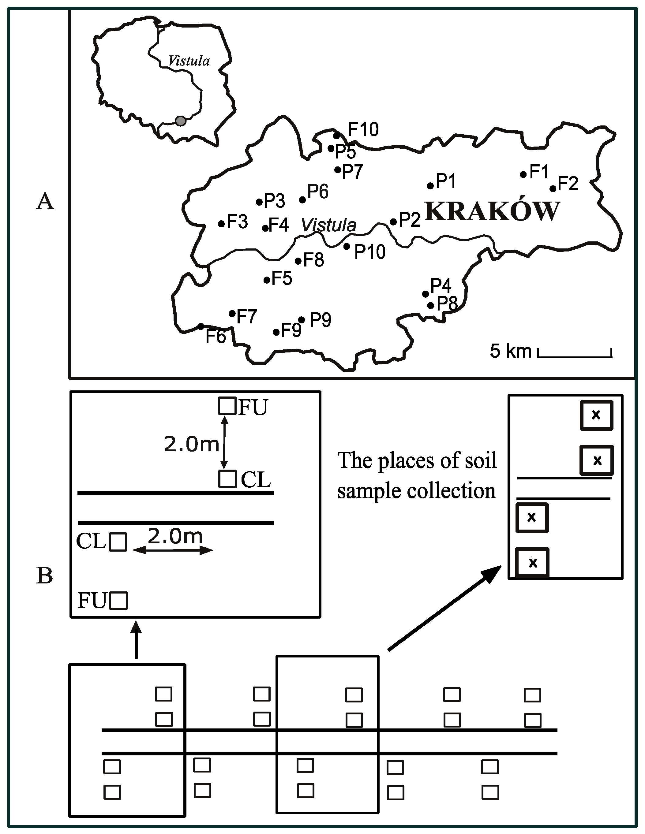
2.1. Study Area and Sampling

The study was carried out in Kraków, southern Poland, in April and May 2022, during the flowering period of spring geophytes (ephemeroids). Kraków covers an area of 327 km2, with a population of 802.6 thousand [38]. It is a Central European city located in the temperate climate zone, with an average annual air temperature of 8.9 °C and an average annual precipitation of 673 mm (data for the period 1991–2020) [38]. A total of 20 sites (10 urban forests and 10 urban parks) were included in the study (Table 1, Figure 1A). In Kraków, forests and parks occupy 4.3% and 1.6% of the city’s total area, respectively, and most of them are easily accessible for residents and tourists [39,40]. The plot sampling followed Kostrakiewicz-Gierałt et al. [36]. In each study site, one representative path was selected, and along each path, 10 pairs of 1 × 1 m plots were sampled. Each pair consisted of a plot, CL (close), located at the edge of the path, and a plot, FU (further), located 2 m from the CL plot (Figure 1B). Altogether, 400 plots were sampled.

2.2. Measurement of Abiotic and Biotic Traits

Field measurements were made during sunny and rainless weather. In the central part of each plot, the light intensity at ground level, soil electrical conductivity and soil compaction were measured (with no repetitions) using the digital light meter Voltcraft Lx-10 (0-199900 lx) (Voltcraft, Hirschau, Germany), soil conductivity tester Hanna GroLine (Hanna Instruments, Olsztyn, Poland) and penetrometer Agreto (Agreto electronics GmbH, Raabs, Austria), respectively. The deeper the penetrometer probe penetrates the soil, the less compact the soil is. In addition, a total of 80 soil samples were collected from the central part of the plots located in the 5th and 6th pair (Figure 1B). Soil collecting followed Kostrakiewicz-Gierałt et al. [36]. The soil samples were dried at room temperature, sieved through a 2 mm sieve and then tested with the Visocolor® kit to determine pH and the content of phosphorus (P), potassium (K), nitrate nitrogen (N-NO3) and ammonium nitrogen (N-NH4).
In each study plot, the percentage of total vegetation cover, the height of the tallest plant and the cover-abundance of individual species of vascular plants in the undergrowth (herb layer) were determined. Thepercentage of total vegetation cover and the height of the tallest plant were measured following Kostrakiewicz-Gierałt et al. [36], whereas the cover-abundance of each species was estimated using the Braun–Blanquet method [41] and following data transformation by Kostrakiewicz-Gierałt et al. [36] as well. The identification of vascular plants was based on the morphological features provided by Csapodý [42], Muller [43] and Rutkowski [44], and the nomenclature was adopted from POWO [45]. Life forms and classification of geophytes followed the BiolFlor database [46,47]. The types of underground storage organs of geophytes were represented by: bulb (B), hypocotyl bulb (HB), rhizome (RH), runner (RU), runner and rhizome (RU-RH), runner-like rhizome (RL-RH), runner and runner with tuberous tip (RU-TU), runner and shoot tuber (RU-ST) and root tuber (RT). The ancient forest species were determined following Dzwonko and Loster [20].

2.3. Statistical Analyses

The normal distribution of the untransformed data was tested using the Kołmogorov–Smirnov test, whereas the homogeneity of variance was verified using the Levene test at the significance level of p < 0.05. Two-way ANOVA analysis followed by the post-hoc Tukey test was performed to check the statistical significance of differences in: (i) light intensity, (ii) soil electrical conductivity, (iii) penetration depth of penetrometer probe, (iv) number of species in herbaceous plant layer, (v) number of geophytes, (vi) share of geophytes in total number of species and (vii) cover-abundance of geophytes between plots CL and FU, as well as between plots located in forests and parks. Moreover, the two-way ANOVA analysis followed by the post-hoc Tukey test were applied to test the statistical significance of differences in: (i) the number of species belonging to RH, RU, RU-RH, RU-TU, HB and RT, (ii) the share of species representing RH, RU, RU-RH, RU-TU, RT, BU and HB, and (iii) the cover-abundance of species representing RU-RH, RT, BU and HB between plots CL and FU, in forests and parks. Due to a lack of homogeneity of variance, the Mann–Whitney U test was applied to check the statistical significance of differences in: (i) total plant cover in the herb layer and (ii) height of the tallest plant shoot in the herb layer between plots CL and FU, and between forests and parks. The aforementioned test was also used to test the statistical significance of differences between plots CL and FU in forests and parks, in the case of: (i) the number of species representing BU, RL-RH and RU-ST, (ii) the share of geophytes belonging to RL-RH and RU-ST, and (iii) the cover-abundance of geophytes representing RH, RU, RL-RH, RU-TU and RU-ST. Moreover, the Mann–Whitney U test was applied to check the statistical significance of differences in the soil reaction and content of P, K, N-NO3 and N-NH4 between plots CL and FU, as well as between forests and parks. The occurrence of a statistically significant correlation between environmental traits (i.e., light intensity, soil electrical conductivity, penetration depth of penetrometer probe, height of the tallest plant shoot, total plant cover and total number of species in herb layer) and the number, share and cover-abundance of geophytes with different underground storage organs was tested using the Pearson coefficient at significance level p ≤ 0.05. The occurrence of a statistically significant correlation between soil properties (i.e., pH, content of P, K, N-NO3 and N-NH4) and number, share and cover-abundance of geophytes with different underground storage organs in plots CL and FU was tested using the Spearman coefficient at significance level p ≤ 0.05. However, we only included the results of correlations for two groups of geophytes, which were characterized by the highest mean values of the number, share and cover-abundance of species. The statistical analyses were performed using the STATISTICA software (version 13.3).

3. Results

3.1. Characteristics of Abiotic Conditions

The light intensity was significantly higher in plots CL than FU (F = 4.17; p ≤ 0.05), but it did not differ significantly between forests and parks. The soil electrical conductivity did not differ significantly between plots CL and FU, as well as between forests and parks. The soil compaction was significantly lower in plots FU than CL (F = 50.12; p < 0.001), as well as in forests than in parks (F = 47.87; p < 0.001). Moreover, the statistical analysis confirmed the occurrence of an interactive effect of the study site and plot (F = 8.79; p < 0.01). The Tukey test showed the presence of significant differences in soil compaction between all plots excluding plots CL in forests and FU in parks. The soil pH and content of ammonium nitrogen (N-NH4), potassium (K) and phosphorus (P) in the soil did not differ significantly between plots CL and FU, as well as between forests and parks. However, the content of nitrate nitrogen (N-NO3) was significantly higher in forests than in parks (U = 107.5; p ≤ 0.05 for plots CL, U = 87.5, p < 0.01 for plots FU). The mean values of abiotic traits are presented in Table 2.

3.2. Characteristics of Plant Cover and Number of Species

The total plant cover in the herb layer was significantly higher in plots FU than CL in parks (Z = −2.50, p ≤ 0.05), whereas it did not differ between plots CL and FU in forests, as well as between forests and parks. The height of the tallest shoot was significantly greater in plots FU than in CL in forests (Z = −4.46, p < 0.001) and parks (Z = −3.12, p < 0.01), as well as in forests than in parks (Z = 3.74, p < 0.001 for plots CL; Z = 5.10, p < 0.001 for plots FU). The number of species in the herb layer was significantly higher in parks than in forests (F = 93.31, p < 0.001). At the same time, the ANOVA analysis confirmed the presence of an interactive effect between the site and plot (F = 4.24, p ≤ 0.05). The Tukey test showed that the number of species noticed in plots CL and FU in forests was significantly lower than the number of species noticed in plots CL and FU in parks. The mean values of plant cover parameters and number of species are presented in Table 3.

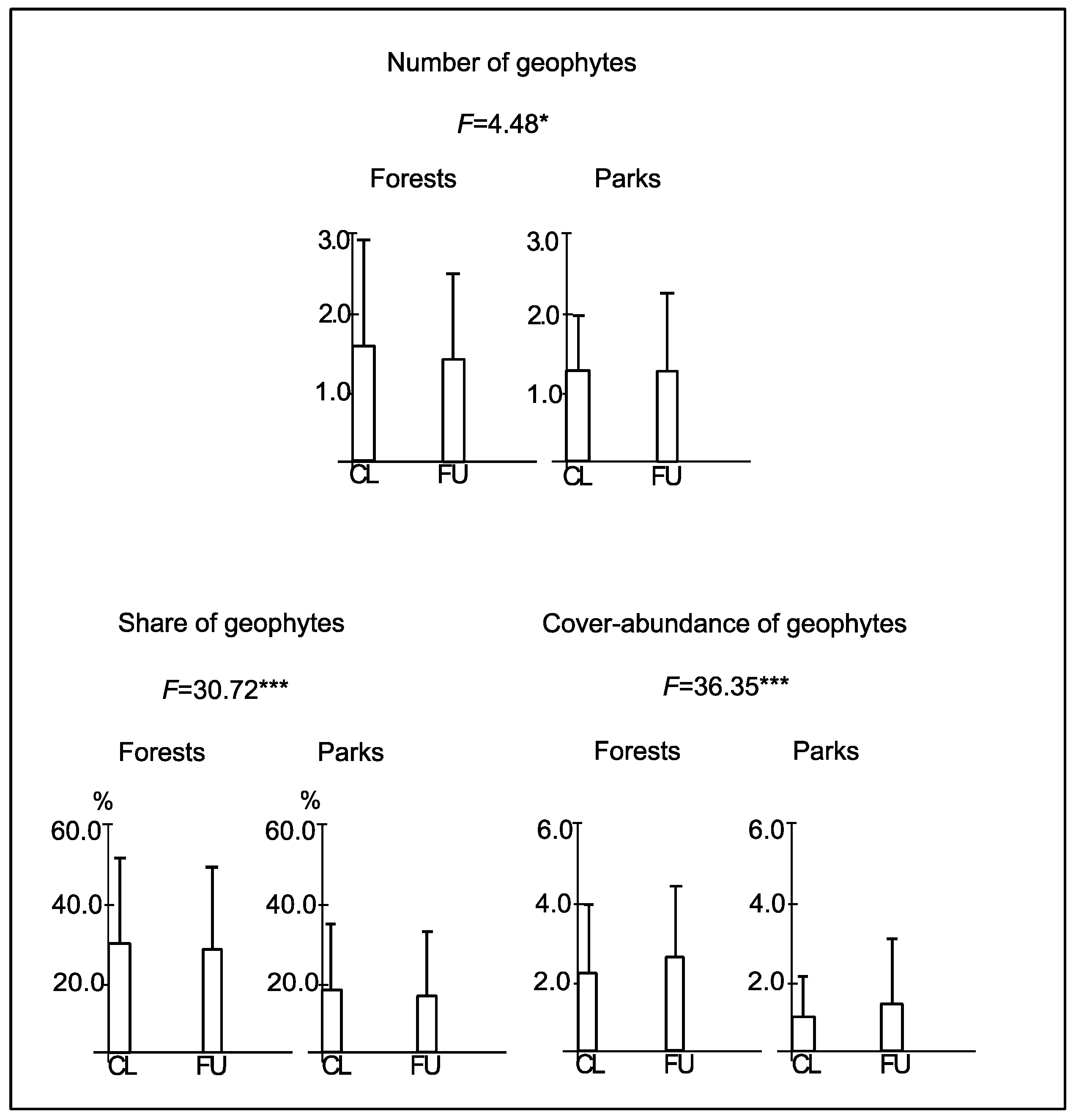
3.3. Characteristics of Geophytes

A total of 23 species of geophytes were recorded, including six species forming the rhizomes, five species forming the runners, four species forming the bulbs, two species forming the runners and rhizomes, two species forming runner-like rhizomes, one species forming the hypocotyl bulbs, one species forming the runners and runners with tuberous tip, one species forming the runners and shoot tubers, and one species forming the root tubers (Table 4). Moreover, there were 14 species typical of ancient forests, and Ranunculus ficaria L. was the most frequent geophyte in study plots (Table 4).
The total number, share and cover-abundance of geophytes were significantly higher in forests than in parks (F = 4.48, p ≤ 0.05; F = 30.72, p < 0.001; F = 36.35, p < 0.001, respectively) but these parameters did not differ between plots CL and FU (Figure 2).
The number, the share and the cover-abundance of species in groups of geophytes are presented in Table 5, Table 6 and Table 7, respectively. The differences in these parameters between plots CL and FU were statistically insignificant, contrary to our first hypothesis. However, we found significant differences in the number, share and cover-abundance of some groups of geophytes between forests and parks. Therefore, our second hypothesis cannot be fully rejected. The groups of geophytes forming the rhizomes (F = 51.45, p < 0.001), runners and rhizomes (F = 8.48, p < 0.01), and runners and runners with tuberous tip (F = 32.34, p < 0.001) were significantly richer in species in forests than in parks. The inversed trend was found in geophytes forming the runners (F = 5.53, p ≤ 0.05) and bulbs, particularly in plots CL (Z = 2.32, p ≤ 0.05). In other cases, the differences were statistically insignificant.
The groups of geophytes with rhizomes (F = 45.87, p < 0.001), runners and rhizomes (F = 13.96, p < 0.001), runners and runners with tuberous tip (F = 23.33, p < 0.001), as well as with root tubers (F = 9.53, p < 0.01) showed significantly higher shares in forests than in parks, whereas the group of geophytes with bulbs achieved a significantly higher share in parks than in forests (F = 6.48, p ≤ 0.05). In other cases, the differences were statistically insignificant.
The groups of geophytes forming the rhizomes (Z = 3.24, p < 0.01 in plots CL; Z = 3.88, p < 0.001 in plots FU), runners and rhizomes (F = 11.86, p < 0.001), and root tubers (F = 5.87, p ≤ 0.05) showed a significantly higher cover-abundance in forests than in parks. In contrast, geophytes forming the bulbs showed a higher cover-abundance in parks than in forests (F = 14.96, p < 0.001). The cover-abundance of other groups of geophytes did not differ significantly between forests and parks.

3.4. The Relationship between the Number of Geophytes and Habitat Conditions

The number of rhizomatous geophytes was correlated with all the environmental traits, except the soil pH and content of N-NH4 (Table 8). Notably, in both CL and FU plots, the number of rhizomatous geophytes was positively correlated with the total number of species in forests, as well as with the penetration depth of the penetrometer probe in parks. Moreover, the content of N-NO3 had the opposite effect on the richness of rhizomatous geophytes between plots CL and FU in forests (Table 8).
The number of root-tuberous geophytes was correlated with all the environmental traits, except the soil pH (Table 8). In both CL and FU plots, it was positively correlated with the total plant cover in forests, and negatively correlated with the height of the herb layer in parks (Table 8).

3.5. The Relationship between the Share of Geophytes and Habitat Conditions

The share of rhizomatous geophytes was correlated with all the environmental traits, except the content of N-NH4 and potassium. In both types of plots, in forests, it was positively correlated with the total number of species and negatively correlated with the content of phosphorus, whereas in parks, it was negatively correlated with the total number of species (Table 9).
The share of root-tuberous geophytes was correlated with all the environmental traits, except the content of N-NH4. In both types of plots, it was negatively correlated with the height of the herb layer and the total number of species in forests and parks, and positively correlated with the penetration depth of the penetrometer probe in parks (Table 9).

3.6. The Relationship between the Cover-Abundance of Geophytes and Habitat Conditions

The cover-abundance of rhizomatous geophytes was correlated with all the environmental traits, except the content of N-NH4. In forests, in both types of plots, it was positively correlated with the total plant cover and total number of species (Table 10).
The cover-abundance of root-tuberous geophytes was correlated with all the environmental traits, except the content of N-NH4, phosphorus and potassium (Table 10). In forests and parks, in both types of plots, it was positively correlated with the penetration depth of the penetrometer probe and negatively correlated with the height of the herb layer and total number of species. Moreover, in both types of plots, it was positively correlated with the light intensity in parks and total plant cover in forests (Table 10).

4. Discussion

Although the CL and FU plots differed significantly in terms of light intensity, soil compaction and height of the herb layer, they were statistically similar in the number, share and cover-abundance of geophytes. Most likely the distance between the CL and FU plots was too short to find significant differences in geophyte characteristics. Nevertheless, Vakhlamova et al. [33] showed that recreation disturbance (trampling and damage to ground vegetation, trees and shrubs), as well as the distance from the forest edge to the nearest road, has no significant effect on the relative abundance of geophytes in urban forests, in contrast to suburban forests. Moreover, Zielińska [48] evidenced that in suburban forests, the number of geophytes is higher near paths than away from them, while the percentage of geophytes shows an inverse relationship. Additionally, Avon et al. [49] documented that forest species (including geophytes) are favored by environmental conditions in the deeper parts of the forests, away from roads. Given this, it can be suggested that the type of forest vegetation, its naturalness or the degree of transformation may have a significant impact on the number, percentage and abundance of geophytes in the distance gradient from the paths. It is also worth noting that the width of the path, the way the path is made (formal or informal, with natural or artificial surface) and the intensity of use of the path are important factors shaping the effect of the distance from the path on forest vegetation [8,32,49,50].
In this study, most of the recorded geophytes were species typical of temperate deciduous forests [51,52] or species characteristic of ancient forests [20,53], so their greater number, share and cover-abundance in forests than in parks is not surprising. Although manor parks can be a refuge for ancient forest species [34], the occurrence of forest geophytes in urban parks is usually negatively affected by low tree density, high fluctuations in temperature and humidity, as well as by regular mowing and intensive trampling [36,50]. The substantial cover-abundance of rhizomatous geophytes in forests can be explained by environmental conditions allowing them high vegetative propagation [54,55,56,57] and seedling recruitment [58,59]. Similarly, Ranunculus ficaria forms dense patches by producing not only underground tuberous roots but also aerial bulblets, which can be dispersed by animals, humans and water [60,61]. Moreover, it is a strong competitor to many spring ephemerals because it appears earlier in the season, uses light efficiently and grows fast [60].
We showed that the more compacted the soil along the paths in forests and parks, the lower the number, share and cover-abundance of rhizomatous geophytes, as well as the lower cover-abundance of R. ficaria. This suggests that rhizomatous and root-tuberous geophytes are particularly susceptible to mechanical damage by trampling. A similar negative effect of trampling was observed by Rusterholz et al. [62] in the case of Anemonoides nemorosa (L.) Holub and R. ficaria in suburban beech forests. Moreover, Littlemore and Barker [63] documented that the rhizomatous geophyte Pteridium aquilinum (L.) Kuhn is less resistant to trampling than the bulbous geophyte Hyacinthoides non-scripta (L.) Chouard ex Rothm. in urban forests.
The increase in light intensity and soil pH had a negative effect on the number, share and cover-abundance of rhizomatous geophytes in the close vicinity of paths in urban forests. Most of the recorded species of rhizome-producing geophytes prefer partial shade and moderately acidic or neutral soil conditions [64]. Although some rhizomatous geophytes show a wide tolerance to soil reactions, in many cases, pH changes can significantly reduce seed germination, population size or biomass. For example, Depauw et al. [65] showed that the germination rate of A. nemorosa is impacted by an interactive effect between light and soil reaction, with negative effects at low and positive effects at high soil pH. Moreover, Baeten et al. [66,67] and Thomaes et al. [68] evidenced that populations of A. nemorosa are threatened by excessive soil acidification. On the other hand, Tyler [69], as well as Falkengren-Grerup and Tyler [70], documented that Convallaria majalis L. prefers a low soil pH and can even grow in acidic raw humus appearing in beech forests, while in sites with a high soil pH, the abundance of individuals diminishes. According to Marrs and Watt [71], P. aquilinum occurs mostly in moderately acidic soils; however, it can also grow in low-alkaline soils. Furthermore, Amouzgar et al. [72] showed that the frond density and biomass of P. aquilinum are negatively correlated with increasing soil pH. Since not all of the investigated paths had a natural surface (Table 1), it is worth emphasizing that using artificial materials to build or harden paths can change the soil pH near paths, which in turn can adversely influence the plant species composition. Interestingly, Godefroid and Koedam [73] documented that the low acidic soil in the close vicinity of paths made of dolomite is significantly greater than near paths covered by cobblestones, asphalt, sand and bare soil, and the number of geophytes decreases successively from a surface made of cobblestones and dolomite, via asphalt and bare soil, to sand in forests. Similarly, Avon et al. [49] evidenced that the limestone gravel used in the construction of roads in forests modifies the acidity of adjacent soils leading to colonization by basophilous plants and avoidance by acidophilous plants along the roads. Moreover, the soil pH can be affected not only by the distance from the path but also by its width [8].
The performed investigations showed that the increasing content of nutrients (N-NO3 and phosphorus) decreases the number, share and cover-abundance of rhizomatous geophytes in the close vicinity of paths in urban forests. In this group of geophytes, the recorded species are typical of mesotrophic or eutrophic soil conditions [64]. According to Godefroid and Koedam [73], the presence of a path leads to an increase in nitrogen-demanding species. Eutrophication of the soil along paths can result from illegal garbage disposal [74] and dog urine [75,76]. Interestingly, Falkengren-Grerup [77] evidenced that the increase in nitrogen availability can decrease the cover, biomass, shoot length and flower frequency of A. nemorosa. Moreover, Gordon et al. [78] documented that nitrogen supplementation leads to earlier sprouting of above-ground parts of P. aquilinum in spring; however, this effect is short-term, and the added nitrogen is preferentially allocated to the rhizomes. On the other hand, Amouzgar et al. [72] showed that frond density and biomass in populations of P. aquilinum are positively correlated with the content of nitrogen and phosphorus in the soil. Furthermore, in plots FU in parks, the number, share and cover-abundance of rhizomatous geophytes were negatively affected by the content of potassium. These findings do not support the observations of Falkengren-Grerup et al. [79] who evidenced a lack of correlation between potassium concentration in the soil solution and the cover of A. nemorosa.
The share and cover-abundance of R. ficaria near the paths in urban parks were positively affected by light intensity and the content of N-NO3 in the soil, and negatively affected by the height of the herb layer and total number of species. According to Zarzycki et al. [64], R. ficaria usually grows in places with partial shade or moderate light, with fertile soil. Moreover, Kermack and Rauschert [80] documented that the abundance and vegetative reproduction of R. ficaria can be influenced by inclination, soil texture, moisture, pH and cation exchange capacity. We assumed that trampling (if it is not too intensive) may favor the expansion of R. ficaria in urban forests and parks since its bulblets easily detach from the maternal plants and can be carried on shoes [61]. However, the effect of trampling intensity in urban forests and parks on geophyte survival and dispersal requires further research.

5. Conclusions

Urban forests and parks can be occupied by various geophytes, including species characteristic of ancient forests. However, the cover-abundance of geophytes producing rhizomes, runners and rhizomes, and root tubers is greater in forests than in parks, in contrast to geophytes producing bulbs. High soil compaction near paths as a result of trampling negatively affects the number, share and cover-abundance of rhizomatous geophytes and the share and cover-abundance of Ranunculus ficaria, the root-tuberous geophyte. To better protect the forest geophytes in urban areas, attention should be paid to limiting trampling and soil eutrophication, as well as preventing excessive increases in soil pH.

Author Contributions

Conceptualization, K.K.-G. and A.P.; methodology, K.K.-G. and A.P.; formal analysis, K.K.-G. and A.P.; investigation, K.K.-G., K.G. and A.P.; resources, K.K.-G. and A.P.; data curation, K.K.-G.; writing—original draft preparation, K.K.-G., K.G. and A.P.; writing—review and editing, K.K.-G., K.G. and A.P.; visualization, K.K.-G. and A.P.; supervision, K.K.-G.; project administration, K.K.-G.; funding acquisition, K.K.-G. All authors have read and agreed to the published version of the manuscript.

Funding

The investigations were financially supported by the Academy of Physical Education in Kraków (project number 292/BS/IT/2022).

Data Availability Statement

Data are contained within the article.

Acknowledgments

The authors thank Zbigniew Gierałt Eng. for his assistance in conducting the field studies and soil analyses.

Conflicts of Interest

The authors declare no conflict of interest.

References

  1. Smaniotto Costa, C.; Šuklje Erjavec, I.; Mathey, J. Green spaces—A key resources for urban sustainability The Green Key sapproach for developing greenspaces. Urbani Izziv. 2008, 19, 199–211. [Google Scholar] [CrossRef]
  2. World Health Organization. Urban Green Spaces: A Brief for Action; World Health Organization, Regional Office for Europe: Copenhagen, Denmark, 2017; p. 24. Available online: https://www.euro.who.int/__data/assets/pdf_file/0010/342289/Urban-Green-Spaces_EN_WHO_web3.pdf (accessed on 11 November 2023).
  3. Cavender, N.; Donnelly, G. Intersecting urban forestry and botanical gardens to address big challenges for healthier trees, people, and cities. Plants People Planet 2019, 1, 315–322. [Google Scholar] [CrossRef]
  4. Pearlmutter, D.; Calfapietra, C.; Samson, R.; O’Brien, L.; Krajter Ostoić, S.; Giovanni Sanesi, G.; del Amo, R.A. (Eds.) The Urban Forest. Future City; Springer: Cham, Switzerland, 2017; Volume 7, p. 351. [Google Scholar] [CrossRef]
  5. Lüttge, U.; Buckeridge, M. Trees: Structure and function and the challenges of urbanization. Trees 2020, 37, 9–16. [Google Scholar] [CrossRef]
  6. Pataki, D.E.; Alberti, M.; Cadenasso, M.L.; Felson, A.J.; McDonnell, M.J.; Pincetl, S.; Pouyat, R.V.; Setälä, H.; Whitlow, T.H. The Benefits and Limits of Urban Tree Planting for Environmental and Human Health. Front. Ecol. Evol. 2021, 9, 603757. [Google Scholar] [CrossRef]
  7. Seymour, M.; Byrne, J.; Martino, D.; Wolch, J. Green Visions Plan for 21st Century Southern California: A Guide for Habitat Conservation, Watershed Health, and Recreational Open Space. 9. Recreationist-Wildlife Interactions in Urban Parks; University of Southern California GIS Research Laboratory and Center for Sustainable Cities: Los Angeles, CA, USA, 2006; p. 87. [Google Scholar]
  8. Zdanowicz, E.; Skłodowski, J. Ocena zmian w środowisku wokół szlaków rekreacyjnych na przykładzie rezerwatu Las Bielański w Warszawie. Stud. I Mater. CEPL W Rogowie 2013, 37, 348–355. [Google Scholar]
  9. Verlič, A.; Arnberger, A.; Japelj, A.; Simončič, P.; Pirnat, J. Perceptions of recreational trail impacts on an urban forest walk: A controlled field experiment. Urban For. Urban Green. 2015, 14, 89–98. [Google Scholar] [CrossRef]
  10. Sujetovienė, G.; Baranauskienė, T. Impact of visitors on soil and vegetation characteristics in urban parks of central Lithuania. Environ. Res. Eng. Manag. 2016, 72, 51–58. [Google Scholar]
  11. Talal, M.L.; Santelmann, M.V. Vegetation management for urban park visitors: A mixed methods approach in Portland, Oregon. Ecol. Appl. 2020, 30, e02079. [Google Scholar] [CrossRef] [PubMed]
  12. Hamzah, H.; Shaari, S.J.; Shamsuddin, M.S. Assessment of Tree Vandalism Level in Kuala Kangsar Urban Park, Perak, Malaysia. Int. J. Acad. Res. Bus. Soc. Sci. 2022, 12, 39–49. [Google Scholar] [CrossRef]
  13. Dafni, A.; Cohen, D.; Noy-Mier, I. Life-cycle variation in geophytes. Ann. Mo. Bot. Gard. 1981, 68, 652–660. [Google Scholar] [CrossRef]
  14. Rundel, P.W.; Anderson, M.K. What is a geophyte? Fremontia 2016, 44, 5–6. [Google Scholar]
  15. Howard, C.C.; Folk, R.A.; Beaulieu, J.M.; Cellinese, N. The monocotyledonous underground: Global climatic and phylogenetic patterns of geophyte diversity. Am. J. Bot. 2019, 106, 850–863. [Google Scholar] [CrossRef] [PubMed]
  16. Tribble, C.M.; Martínez-Gómez, J.; CoyoteeHoward, C.; Males, J.; Sosa, V.; Sessa, E.B.; Cellinese, N.; Specht, C.D. Get the shovel: Morphological and evolutionary complexities of belowground organ sin geophytes. Am. J. Bot. 2021, 108, 372–387. [Google Scholar] [CrossRef]
  17. Noy-Meir, I.; Oron, T. Effects of grazing on geophytes in Mediterranean vegetation. J. Veg. Sci. 2001, 12, 749–760. [Google Scholar] [CrossRef]
  18. Popović, Z.; Vidaković, V. Ecophysiological and growth-related traits of two geophytes three years after the fire event in grassland steppe. Plants 2022, 11, 734. [Google Scholar] [CrossRef]
  19. Khosa, J.; Bellinazzo, F.; Kamenetsky Goldstein, R.; Macknight, R.; Immink, R.G.H. Phosphatidylethanolamine-Binding Proteins: The conductors of dual reproduction in plants with vegetative storage organs. J. Exp. Bot. 2021, 72, 2845–2856. [Google Scholar] [CrossRef]
  20. Dzwonko, Z.; Loster, S. Wskaźnikowe gatunki roślin starych lasów i ich znaczenie dla ochrony przyrody i kartografii roślinności. Prace Geogr. 2001, 178, 119–132. [Google Scholar]
  21. Sikorska, D.; Sikorski, P.; Wierzba, M. Ancient forest species in tree stands of different age as indicators of the continuity of forest habitat. Ann. Wars. Univ. Life Sci. SGGW Hortic. Landsc. Archit. 2008, 29, 155–162. [Google Scholar]
  22. Jabs-Sobocińska, Z.; Affek, A.N.; Matuszkiewicz, J.M. The list of ancient-forest plant species revisited—Field verification in the Carpathian ancient and recent forests. For. Ecol. Manag. 2022, 512, 120152. [Google Scholar] [CrossRef]
  23. Seyidoğlu, N.; Zencirkıran, M.; Ayaşlıgil, A. Position and application areas of geophytes within landscape design. Afr. J. Agric. Res. 2009, 4, 1351–1357. [Google Scholar]
  24. Nagase, A.; Dunnett, N. Performance of geophytes on extensive green roofs in the United Kingdom. Urban For. Urban Green. 2013, 12, 509–521. [Google Scholar] [CrossRef]
  25. Ros, M.; Garcia, C.; Hernandez, T.; Andres, M.; Barja, A. Short-Term Effects of Human Trampling on Vegetation and Soil Microbial Activity. Commun. Soil Sci. Plant Anal. 2004, 35, 1591–1603. [Google Scholar] [CrossRef]
  26. Dumitraşcu, M.; Marin, A.; Preda, E.; Ţîbîrnac, M.; Vădineanu, A. Trampling effects on plant species morphology. Rom. J. Biol. Plant Biol. 2010, 55, 89–96. [Google Scholar]
  27. Lehvävirta, S.; Vilisics, F.; Hamberg, L.; Malmivaara-Lämsä, M.; Kotze, J.D. Fragmentation and recreational use affect tree regeneration in urban forests. Urban For. Urban Green. 2014, 13, 869–877. [Google Scholar] [CrossRef]
  28. Pescott, O.L.; Stewart, G.B. Assessing the impact of human trampling on vegetation: A systematic review and meta-analysis of experimental evidence. PeerJ 2014, 2, e360. [Google Scholar] [CrossRef]
  29. Jägerbrand, A.K.; Alatalo, J.M. Effects of human trampling on abundance and diversity of vascular plants, bryophytes and lichens in alpine heath vegetation, Northern Sweden. SpringerPlus 2015, 4, 95. [Google Scholar] [CrossRef]
  30. Kuss, F.R. A review of major factors influencing plant responses to recreation impacts. Environ. Manag. 1986, 10, 637–650. [Google Scholar] [CrossRef]
  31. Sun, D.; Liddle, M.J. A survey of trampling effects on vegetation and soil in eight tropical and subtropical sites. Environ. Manag. 1993, 17, 497–510. [Google Scholar] [CrossRef]
  32. Kostrakiewicz-Gierałt, K.; Pliszko, A.; Gmyrek, K. The effect of informal tourist trails on the abiotic conditions and floristic composition of deciduous forest undergrowth in an urban area. Forests 2021, 12, 423. [Google Scholar] [CrossRef]
  33. Vakhlamova, T.; Rusterholz, H.-P.; Kamkin, V.; Baur, B. Recreational use of urban and suburban forests affects plant diversity in a Western Siberian city. Urban For. Urban Green. 2016, 17, 92–103. [Google Scholar] [CrossRef]
  34. Fornal-Pieniak, B.; Ollik, M.; Schwerk, A. Impact of different levels of anthropogenic pressure on the plant species composition in woodland sites. Urban For. Urban Green. 2019, 38, 295–304. [Google Scholar] [CrossRef]
  35. Erfanian, M.B.; Alatalo, J.M.; Ejtehadi, H. Severe vegetation degradation associated with different disturbance types in a poorly managed urban recreation destination in Iran. Sci. Rep. 2021, 11, 19695. [Google Scholar] [CrossRef] [PubMed]
  36. Kostrakiewicz-Gierałt, K.; Gmyrek, K.; Pliszko, A. The effect of the distance from a path on abiotic conditions and vascular plant species in the undergrowth of urban forests and parks. Int. J. Environ. Res. Public Health 2022, 19, 5621. [Google Scholar] [CrossRef] [PubMed]
  37. Hagiladi, A.; Umiel, N.; Ozeri, Y.; Elyasi, R.; Abramsky, S.; Levy, A.; Lobovsky, O.; Matan, E. The effect of planting depth on emergence and development of some geophytic plants. Acta Hortic. 1992, 325, 131–138. [Google Scholar] [CrossRef]
  38. Statistics Poland. Statistical Yearbook of the Republic of Poland; Statistics Poland: Warsaw, Poland, 2022; p. 791.
  39. Municipal Greenery Management in Kraków. 2023. Available online: https://zzm.krakow.pl/zzm/parki.html (accessed on 11 November 2023).
  40. Kwartnik-Pruc, A.; Trembecka, A. Public Green Space Policy Implementation: A Case Study of Krakow, Poland. Sustainability 2021, 13, 538. [Google Scholar] [CrossRef]
  41. Braun-Blanquet, J. Pflanzensoziologie. Grundzüge der Vegetationskunde, 3rd ed.; Springer: Berlin/Heidelberg, Germany, 1964; p. 631. [Google Scholar]
  42. Csapodý, V. Keimlingsbestimmungsbuch der Dikotyledonen; Akademiai Kiado: Budapeszt, Hungary, 1968; p. 286. [Google Scholar]
  43. Muller, F.M. Seedlings of the North-Western European Lowland. In A Flora of Seedlings, 1st ed.; Springer: Wageningen, The Netherlands, 1978; p. 653. [Google Scholar]
  44. Rutkowski, L. Klucz do Oznaczania Roślin Naczyniowych Polski Niżowej; Wydawnictwo Naukowe PWN: Warszawa, Poland, 2004; p. 814. [Google Scholar]
  45. POWO. Plants of the World Online. 2023. Available online: http://www.plantsoftheworldonline.org (accessed on 21 March 2023).
  46. Klotz, S.; Kühn, I.; Durka, W. BIOLFLOR—Eine Datenbankmitbiologisch-ökologischen Merkmalenzur Flora von Deutschland; Bundesamt für Naturschutz: Bonn, Germany, 2002; p. 334.
  47. BiolFlor. BiolFlor, Search and Information System on Vascular Plants in Germany. 2023. Available online: https://www.ufz.de/biolflor/index.jsp (accessed on 20 February 2023).
  48. Zielińska, K. The influence of roads on the species diversity of forest vascular flora in Central Poland. Biodiv. Res. Conserv. 2007, 5–8, 71–80. [Google Scholar]
  49. Avon, C.; Dumas, Y.; Bergès, L. Management practices increase the impact of roads on plant communities in forests. Biol. Conserv. 2013, 159, 24–31. [Google Scholar] [CrossRef]
  50. Sikorski, P.; Szumacher, I.; Sikorska, D.; Kozak, M.; Wierzba, M. Effects of visitor pressure on understory vegetation in Warsaw forested parks (Poland). Environ. Monit. Assess. 2013, 185, 5823–5836. [Google Scholar] [CrossRef]
  51. Mucina, L. Conspectus of classes of European vegetation. Folia Geobot. Phytotax. 1997, 32, 117–172. [Google Scholar] [CrossRef]
  52. Matuszkiewicz, W. Przewodnik do Oznaczania Zbiorowisk Roślinnych Polski; Wydawnictwo Naukowe PWN: Warszawa, Poland, 2008; p. 540. [Google Scholar]
  53. Dzwonko, Z. Rośliny runa wskaźnikami pochodzenia i przemian lasów. Stud. I Mater. CEPL W Rogowie 2015, 42, 27–37. [Google Scholar]
  54. Pirożnikow, E. Demography of Anemone nemorosa L. in dry-site deciduous forest (Tilio-Carpinetum) in the Bialowieza Forest. Ekol. Pol. 1994, 42, 155–172. [Google Scholar]
  55. Kosiński, I. The influence of shoot harvesting on the size and fecundity of Convallaria majalis L. Acta Soc. Bot. Pol. 2001, 70, 303–312. [Google Scholar] [CrossRef]
  56. Vandepitte, K.; DeMeyer, T.; Jacquemyn, H.; Honnay, O.; Roldán-Ruiz, I. The impact of extensive clonal growth on fine-scale mating patterns: A full paternity analysis of a lily-of-the-valley population (Convallaria majalis). Ann. Bot. 2013, 111, 623–628. [Google Scholar] [CrossRef] [PubMed]
  57. Vandepitte, K.; Jacquemyn, H.; Roldán-Ruiz, I.; Honnay, O. Extremely low genotypic diversity and sexual reproduction in isolated populations of the self-incompatible lily-of-the-valley (Convallaria majalis) and the role of the local forest environment. Ann. Bot. 2019, 105, 769–776. [Google Scholar] [CrossRef]
  58. Eriksson, O. Seedling recruitment in deciduous forest herbs: The effects of litter, soil chemistry and seed bank. Flora 1995, 190, 65–70. [Google Scholar] [CrossRef]
  59. Holderegger, R.; Stehlik, I.; Schneller, J.J. Estimation of the relative importance of sexual and vegetative reproduction in the clonal woodland herb Anemone nemorosa. Oecologia 1998, 117, 105–107. [Google Scholar] [CrossRef]
  60. Axtell, A.E.; DiTommaso, A.; Post, A.R. Lesser Calendine (Ranunculus ficaria): A threat to woodland habitats in the northern United States and southern Canada. Invasive Plant Sci. Manag. 2010, 3, 190–196. [Google Scholar] [CrossRef]
  61. Sohrabi Kertabad, S.; Rashed Mohassel, M.H.; Nasiri Mahalati, M.; Gherekhloo, J. Some biological aspects of the weed Lesser celandine (Ranunculus ficaria). Planta Daninha 2013, 31, 577–585. [Google Scholar] [CrossRef]
  62. Rusterholz, H.-P.; Weisskopf-Kissling, M.; Baur, B. Single versus repeated human trampling events: Responses of ground vegetation in suburban beech forests. Appl. Veg. Sci. 2021, 24, e12604. [Google Scholar] [CrossRef]
  63. Littlemore, J.; Baker, S. The ecological response of forest ground flora and soils to experimental trampling in British urban woodlands. Urban Ecosyst. 2001, 5, 257–276. [Google Scholar] [CrossRef]
  64. Zarzycki, K.; Trzcińska-Tacik, H.; Różański, W.; Szeląg, Z.; Wołek, J.; Korzeniak, U. Ecological Indicator Values of Vascular Plants of Poland; W. Szafer Institute of Botany, Polish Academy of Sciences: Kraków, Poland, 2002; p. 183. [Google Scholar]
  65. Depauw, L.; Hu, R.; Dhungana, K.S.; Govaert, S.; Meeussen, C.; Vangansbeke, P.; Strimbeck, R.; Graae, B.J.; De Frenne, P. Functional trait variation of Anemone nemorosa along macro-and microclimatic gradients close to the northern range edge. Nord. J. Bot. 2022, 2022, e03471. [Google Scholar] [CrossRef]
  66. Baeten, L.; Bauwens, B.; De Schrijver, A.; De Keersmaeker, L.; Van Calster, H.; Vandekerkhove, K.; Roelandt, B.; Beeckman, H.; Verheyen, K. Compositional changes (1954–2000) in the forest herb layer following the cessation of coppice –with –standards management and soil acidification. Appl. Veg. Sci. 2009, 12, 187–197. [Google Scholar] [CrossRef]
  67. Baeten, L.; DeFrenne, P.; Verheyen, K.; Graae, B.J.; Hermy, M. Forest herbs in the face of global change: A single –species –multiple –threats approach for Anemone nemorosa. Plant Ecol. Evol. 2010, 143, 19–30. [Google Scholar] [CrossRef]
  68. Thomaes, A.; DeKeersmaeker, L.; DeSchrijver, A.; Baeten, L.; Vandekerkhove, K.; Verstraeten, G.; Verheyen, K. Can soil acidity and light help to explain tree species effects on forest herb layer performance in post-agricultural forests? Plant Soil 2013, 373, 183–199. [Google Scholar] [CrossRef]
  69. Tyler, G. Interacting effects of soil acidity and canopy cover on the species composition of field- layer vegetation in oak/hornbeam forests. For. Ecol. Manag. 1989, 28, 101–114. [Google Scholar] [CrossRef]
  70. Falkengren-Grerup, U.; Tyler, G. Soil chemical properties excluding field-layers pecies from beech forest mor. Plant Soil 1993, 148, 185–191. [Google Scholar] [CrossRef]
  71. Marrs, R.M.; Watt, A.S. Biological flora of the British Isles: Pteridium aquilinum (L.) Kuhn. J. Ecol. 2006, 94, 1272–1321. [Google Scholar] [CrossRef]
  72. Amouzgar, L.; Ghorbani, J.; Shokri, M.; Marrs, R.H.; Alday, J.G. Pteridium aquilinum performance is driven by climate, soil and land-use in Southwest Asia. Folia Geobot. 2020, 55, 301–314. [Google Scholar] [CrossRef]
  73. Godefroid, S.; Koedam, N. The impact of forest paths upon adjacent vegetation: Effects of the path surfacing material on the species composition and soil compaction. Biol. Conserv. 2004, 119, 405–419. [Google Scholar] [CrossRef]
  74. Yang, J.-L.; Zhang, G.-L. Formation, characteristics and eco-environmental implications of urban soils—A review. Soil Sci. Plant Nutr. 2015, 61, 30–46. [Google Scholar] [CrossRef]
  75. Paradeis, B.; Lovas, S.; Aipperspach, A.; Kazmierczak, A.; Boche, M.; He, Y.; Corrigan, P.; Chambers, K.; Gao, Y.; Norland, J.; et al. Dog-park soils: Concentration and distribution of urine-borne constituents. Urban Ecosyst. 2013, 16, 351–365. [Google Scholar] [CrossRef]
  76. Allen, J.A.; Setälä, H.; Kotze, D.J. Dog urine has acute impacts on soil chemistry in urban green spaces. Front. Ecol. Evol. 2020, 8, 615979. [Google Scholar] [CrossRef]
  77. Falkengren-Grerup, U. Effects on beech forest species of experimentally enhanced nitrogen deposition. Flora 1993, 188, 85–91. [Google Scholar] [CrossRef]
  78. Gordon, C.; Woodin, S.J.; Alexander, I.J.; Mullins, C.E. Effects of increased temperature, drought and nitrogen supply on two upland perennials of contrasting functional type: Calluna vulgaris and Pteridium aquilinum. New Phytol. 1999, 142, 243–258. [Google Scholar] [CrossRef]
  79. Falkengren-Grerup, U.; Quist, M.E.; Tyler, G. Relative importance of exchangeable and soil solution cations concentrations to the distribution of vascular plants. Environ. Exp. Bot. 1995, 35, 9–15. [Google Scholar] [CrossRef]
  80. Kermack, J.P.; Rauschert, E. Soil characteristics drive Ficaria verna abundance and reproductive output. Invasive Plant Sci. Manag. 2019, 12, 214–222. [Google Scholar] [CrossRef]
Figure 1. Distribution of study sites in Kraków, southern Poland (A), and sampling scheme (B). The symbols of study sites are explained in Table 1. CL means the plot located close to the path and FU means the plot located far from the path.
Forests 14 02272 g001
Figure 2. Differences in total number, share and cover-abundance of geophytes between closer (CL) and further (FU) plots located along the paths in forests and parks (Kraków, Poland). The asterisks show the statistical significance of differences at levels p ≤ 0.05 (*) and p < 0.001 (***).
Forests 14 02272 g002
Table 1. List of study sites (Kraków, Poland) with their characteristics.
Study SiteSymbolGPS CoordinatesElevation
(m a.s.l.)
Width of the Path (cm)Type of Path Surface
Łęgowski ForestF1N 50°03.116′199300artificial (gravel)
E 20°02.092′
Mogilski ForestF2N 50°03.228′200285artificial (asphalt)
E 20°03.195′
Wolski ForestF3N 50°03.336′334160natural
E 19°51.445′
Forest in Sikornik HillF4N 50°03.466′286101natural
E 19°53.175′
Forest in Górka PychowickaF5N 50°01.908′252215natural
E 19°52.967′
Tyniec ForestF6N 50°00.641′245260natural
E 19°49.709′
Forest in SkotnikiF7N 50°01.250′218200artificial (gravel)
E 19°51.118′
Forest of Twardowski
Rocks
F8N 50°02.521′234305natural
E 19°54.546′
Borkowski ForestF9N 50°00.666′215130natural
E 19°54.748′
Witkowice ForestF10N 50°06.475′238100natural
E 19°57.000′
Polish Aviator’s ParkP1N 50°04.371′229175artificial (asphalt)
E 19°59.424′
Dąbie ParkP2N 50°03.579′202120natural
E 19°58.978′
Decius ParkP3N 50°03.957′256225artificial (asphalt)
E 19°52.379′
Anna and Erazm Jerzmanowski ParkP4N 50°01.030′219182artificial (sand and gravel)
E 19°59.657′
Stanisław Wyspiański’s
Park
P5N 50°05.135′235300artificial (asphalt)
E 19°55.284′
Henryk Jordan’s ParkP6N 50°03.742′204310artificial (asphalt)
E 19°54.996′
Kleparski ParkP7N 50°04.583′222300artificial (asphalt)
E 19°56.241′
Aleksandra’s ParkP8N 50°00.727′22390natural
E 20°00.881′
Solvay ParkP9N 50°00.916′226175natural
E 19°55.599′
Florian Nowacki’s
Park
P10N 50°02.625′178168artificial (sett)
E 19°56.577′
Table 2. Comparison of abiotic traits (mean and SD) between closer (CL) and further (FU) plots located along the paths in forests and parks (Kraków, Poland).
Abiotic TraitsForestsParks
CLFUCLFU
Light intensity at ground level (lx)10,508.41 (±19,251.41)6449.63 (±13,293.03)11,940.01 (±15,231.39)9856.61 (±11,143.89)
Soil electrical conductivity (mS/cm)0.15 (±0.14)0.17 (±0.18)0.15 (±0.15)0.13 (±0.10)
Penetration depth of the penetrometer probe (cm)24.10 (±19.95)43.81 (±21.42)16.34 (±15.33)24.41 (±21.17)
Soil pH6.70 (±0.38)6.57 (±0.49)6.67 (±0.44)6.37 (±0.72)
Content of N-NH4 (mg/kg)23.99 (±70.73)16.38 (±38.54)3.90 (±6.33)3.71 (±6.26)
Content of N-NO3 (mg/kg)66.70 (±25.47)57.50 (±11.70)43.12 (±29.81)33.93 (±25.64)
Content of K (mg/kg)58.00 (±66.35)65.50 (±71.34)38.50 (±46.86)25.80 (±29.34)
Content of P (mg/kg)18.00 (±17.12)13.00 (±14.09)22.25 (±19.23)16.25 (±17.98)
Table 3. Comparison of biotic traits (mean and SD) between closer (CL) and further (FU) plots located along the paths in forests and parks (Kraków, Poland).
Biotic TraitsForestsParks
CLFUCLFU
Total plant cover (%)32.85 (±23.56)36.94 (±29.19)33.10 (±21.06)41.55 (±25.85)
Height of the tallest shoot in herb layer (cm)36.32 (±23.39)51.60 (±26.39)25.51 (±16.90)34.21 (±22.35)
Number of species5.64 (±2.41)4.64 (±2.12)7.91 (±3.34)8.14 (±3.77)
Table 4. List of geophytes recorded in closer (CL) and further (FU) plots in forests and parks in Kraków, southern Poland. Ancient forest species are bolded.
SpeciesAbbreviation of GroupStorage OrganMean Frequency of Occurrence
ForestsParks
CLFUCLFU
Allium oleraceum L.BUbulb-0.10 (±0.32)0.10 (±0.32)0.30 (±0.95)
Anemonoides nemorosa (L.) HolubRHrhizome3.10 (±4.20)3.80 (±4.44)0.30 (±0.95)0.60 (±1.58)
Anemonoides ranunculoides (L.) HolubRHrhizome--0.30 (±0.95)0.40 (±1.26)
Carex brizoides L.RU-RHrunner, rhizome1.10 (±3.14)0.90 (±2.85)--
Carex hirta L.RU-RHrunner, rhizome0.20 (±0.63)-0.40 (±0.97)0.30 (±0.67)
Circaea lutetiana L.RU-TUrunner, runner with tuberous tip1.50 (±2.17)1.20 (±2.39)--
Convallaria majalis L.RHrhizome0.40 (±1.26)0.70 (±2.21)--
Corydalis solida (L.) Clairv.HBhypocotyl bulb1.00 (±2.83)0.50 (±1.58)0.10 (±0.32)0.10 (±0.32)
Elymus repens (L.) GouldRL-RHrunner-like rhizome--0.30 (±0.67)-
Equisetum arvense L.RU-STrunner, shoot tuber--0.10 (±0.32)-
Gagea lutea (L.) Ker Gawl.BUbulb0.10 (±0.32)0.10 (±0.32)1.90 (±3.11)2.30 (±3.74)
Galium odoratum (L.) Scop.RUrunner0.40 (±1.26)0.40 (±0.97)--
Glechoma hederacea L.RUrunner0.70 (±1.34)0.60 (±1.35)2.70 (±2.87)3.00 (±2.45)
Lathyrus vernus (L.) Bernh.RHrhizome-0.10 (±0.32)--
Lilium martagon L.BUbulb0.50 (±1.58)0.30 (±0.95)--
Lysimachia vulgaris L.RUrunner0.10 (±0.32)---
Maianthemum bifolium (L.) F. W. SchmidtRL-RHrunner-like rhizome-0.10 (±0.32)--
Mercurialis perennis L.RUrunner0.70 (±2.21)0.90 (±2.51)--
Ornithogalum umbellatum L.BUbulb---0.19 (±0.51)
Oxalis stricta L.RUrunner0.20 (±0.42)-0.30 (±0.67)0.10 (±0.32)
Polygonatum odoratum (Mill.) DruceRHrhizome0.50 (±1.58)0.30 (±0.95)--
Pteridium aquilinum (L.) KuhnRHrhizome0.10 (±0.32)0.20 (±0.63)--
Ranunculus ficaria L.RTroot tuber5.70 (±4.27)4.20 (±3.94)5.90 (±3.11)5.60 (±3.37)
Table 5. The mean (±SD) number of geophytes with different underground storage organs in closer (CL) and further (FU) plots located along paths in forests and parks (Kraków, Poland). The similar letters in superscripts mean the lack of differences (Tukey test).
Underground Storage OrganForestsParks
CLFUCLFU
Bulb0.03 (±0.17)0.10 (±0.36)0.22 (±0.42)0.23 (±0.42)
Hypocotyl bulb0.06 (±0.24)0.01 (±0.10)0.02 (±0.14)0.04 (±0.20)
Rhizome0.41 (±0.65) a0.47 (±0.64) a0.06 (±0.24) b0.10 (±0.33) b
Runner0.22 (±0.50) a0.18 (±0.44) b0.31 (±0.46) b0.31 (±0.46) b
Runner and rhizome0.13 (±0.34) a0.09 (±0.29) a0.04 (±0.20) b0.03 (±0.17) b
Runner-like rhizome0.00 (±0.00)0.00 (±0.10)0.05 (±0.22)0.00 (±0.00)
Runner and runner with tuberous tip0.16 (±0.37) a0.12 (±0.33) a0.00 (±0.00) b0.00 (±0.00) b
Runner and shoot tuber0.00 (±0.00)0.00 (±0.00)0.01 (±0.10)0.00 (±0.00)
Root tuber0.57 (±0.50)0.42 (±0.50)0.59 (±0.49)0.56 (±0.50)
Table 6. The mean (±SD) share (%) of geophytes with different underground storage organs in closer (CL) and further (FU) plots located along paths in forests and parks (Kraków, Poland). The similar letters in superscripts mean the lack of differences (Tukey test).
Underground Storage OrganForestsParks
CLFUCLFU
Bulb0.39 (±2.31) a1.99 (±7.35) a4.07 (±8.39) b3.61 (±7.27) b
Hypocotyl bulb0.77 (±3.12)0.17 (±1.67)0.23 (±1.69)0.42 (±2.24)
Rhizome6.07 (±9.63) a7.98 (±10.71) a1.19 (±5.22) b1.71 (±6.04) b
Runner3.26 (±7.36)2.89 (±6.92)3.12 (±4.96)3.39 (±5.47)
Runner and rhizome2.48 (±6.80) a1.87 (±6.12) a0.45 (±2.21) b0.32 (±1.84) b
Runner-like rhizome0.00 (±0.00)0.11 (±1.11)0.57 (±2.57)0.00 (±0.00)
Runner and runner with tuberous tip2.55 (±6.26) a2.16 (±6.06) a0.00 (±0.00) b0.00 (±0.00) b
Runner and shoot tuber0.00 (±0.00)0.00 (±0.00)0.14 (±1.43)0.00 (±0.00)
Root tuber14.82 (±20.22) a11.94 (±19.26) a9.57 (±10.06) b7.60 (±7.98) b
Table 7. The mean (±SD) cover-abundance coefficient of geophytes with different underground storage organs in closer (CL) and further (FU) plots located along paths in forests and parks (Kraków, Poland). The similar letters in superscripts mean the lack of differences (Tukey test).
Underground Storage OrganForestsParks
CLFUCLFU
Bulb0.01 (±0.03) a0.02 (±0.11) a0.10 (±0.35) b0.15 (±0.47) b
Hypocotyl bulb0.01 (±0.03)0.01 (±0.10)0.00 (±0.01)0.02 (±0.20)
Rhizome0.62 (±1.10) a0.84 (±1.30) a0.02 (±0.14) b0.10 (±0.39) b
Runner0.10 (±0.38)0.18 (±0.57)0.05 (±0.14)0.14 (±0.43)
Runner and rhizome0.14 (±0.40) a0.14 (±0.47) a0.02 (±0.14) b0.01 (±0.10) b
Runner-like rhizome0.00 (±0.00)0.00 (±0.01)0.02 (±0.20)0.00 (±0.00)
Runner and runner with tuberous tip0.04 (±0.22)0.01 (±0.03)0.00 (±0.00)0.00 (±0.00)
Runner and shoot tuber0.00 (±0.00)0.00 (±0.00)0.00 (±0.01)0.00 (±0.00)
Root tuber1.28 (±1.47) a1.13 (±1.66) a0.75 (±1.01) b1.00 (±1.27) b
Table 8. The values of correlation coefficients between the number of geophytes and environmental traits in plots CL and FU, in forests and parks in Kraków, Poland. Explanations: CL—plots located close to the path, FU—plots located further from the path, RH—geophytes with rhizomes, RT—geophytes with root tubers, LI—light intensity, SEC—soil electrical conductivity, PD—penetration depth of penetrometer probe, HTS—height of the tallest shoot in the herb layer, TPC—total plant cover in the herb layer, TNS—total number of vascular plant species in the herb layer, SR—soil reaction, N-NO3—content of nitrate nitrogen, N-NH4—content of ammonium nitrogen, P—content of phosphorus, K—content of potassium. The statistically significant values at level p ≤ 0.05 are bolded. The values for LI, SEC, PD, HTS, TPC and TNS mean the Pearson coefficient, and in other cases, the Spearman coefficient.
LISECPDHTSTPCTNSSRN-NO3N-NH4PK
ForestsCLRH−0.23−0.080.270.140.210.39−0.42−0.500.11−0.59−0.43
RT0.090.300.17−0.260.20−0.290.300.21−0.300.390.01
FURH−0.12−0.200.13−0.010.170.48−0.420.500.28−0.430.15
RT0.280.180.36−0.320.48−0.080.32−0.25−0.290.18−0.02
ParksCLRH−0.130.130.40−0.19−0.06−0.090.170.21−0.04−0.29−0.17
RT0.230.030.19−0.33−0.07−0.21−0.210.43−0.39−0.010.29
FURH−0.150.130.24−0.200.060.01−0.270.24−0.02−0.16−0.48
RT0.170.290.20−0.330.150.04−0.320.36−0.520.01−0.31
Table 9. The values of correlation coefficients between the share of geophytes and environmental traits in plots CL and FU, in forests and parks in Kraków, Poland. Explanations: CL—plots located close to the path, FU—plots located further from the path, RH—geophytes with rhizomes, RT—geophytes with root tubers, LI—light intensity, SEC—soil electrical conductivity, PD—penetration depth of penetrometer probe, HTS—height of the tallest shoot in the herb layer, TPC—total plant cover in the herb layer, TNS—total number of vascular plant species in the herb layer, SR—soil reaction, N-NO3—content of nitrate nitrogen, N-NH4—content of ammonium nitrogen, P—content of phosphorus, K—content of potassium. The statistically significant values at level p ≤ 0.05 are bolded. The values for LI, SEC, PD, HTS, TPC and TNS mean the Pearson coefficient, and in other cases, the Spearman coefficient.
LISECPDHTSTPCTNSSRN-NO3N-NH4PK
ForestsCLRH−0.230.000.250.160.190.21−0.49−0.540.16−0.60−0.43
RT0.160.120.04−0.380.22−0.610.300.14−0.310.530.04
FURH−0.13−0.280.05−0.090.170.34−0.400.350.14−0.500.02
RT0.240.090.40−0.400.14−0.300.38−0.24−0.330.22−0.05
ParksCLRH−0.100.150.53−0.17−0.01−0.200.170.22−0.04−0.31−0.19
RT0.300.030.24−0.42−0.02−0.53−0.170.45−0.35−0.140.22
FURH−0.160.090.14−0.26−0.04−0.20−0.290.22−0.05−0.14−0.48
RT0.300.200.21−0.390.14−0.30−0.460.27−0.430.08−0.33
Table 10. The values of correlation coefficients between the cover-abundance of geophytes and environmental traits in plots CL and FU, in forests and parks in Kraków, Poland. Explanations: CL—plots located close to the path, FU—plots located further from the path, RH—geophytes with rhizomes, RT—geophytes with root tubers, LI—light intensity, SEC—soil electrical conductivity, PD—penetration depth of penetrometer probe, HTS—height of the tallest shoot in the herb layer, TPC—total plant cover in the herb layer, TNS—total number of vascular plant species in the herb layer, SR—soil reaction, N-NO3—content of nitrate nitrogen, N-NH4—content of ammonium nitrogen, P—content of phosphorus, K—content of potassium. The statistically significant values at level p ≤ 0.05 are bolded. The values for LI, SEC, PD, HTS, TPC and TNS mean the Pearson coefficient, and in other cases, the Spearman coefficient.
LISECPDHTSTPCTNSSRN-NO3N-NH4PK
ForestsCLRH−0.23−0.040.230.200.300.30−0.45−0.520.22−0.63−0.27
RT−0.020.280.23−0.310.58−0.360.370.12−0.400.34−0.24
FURH−0.14−0.250.05−0.050.240.29−0.470.390.39−0.200.27
RT0.210.130.40−0.270.71−0.260.36−0.24−0.320.15−0.02
ParksCLRH−0.090.070.44−0.12−0.03−0.170.140.18−0.01−0.27−0.17
RT0.310.020.30−0.460.15−0.38−0.220.49−0.400.20−0.13
FURH−0.140.160.17−0.140.140.00−0.240.25−0.01−0.17−0.48
RT0.280.200.25−0.390.32−0.20−0.410.30−0.440.05−0.29
Disclaimer/Publisher’s Note: The statements, opinions and data contained in all publications are solely those of the individual author(s) and contributor(s) and not of MDPI and/or the editor(s). MDPI and/or the editor(s) disclaim responsibility for any injury to people or property resulting from any ideas, methods, instructions or products referred to in the content.

