Abstract
Deadwood is a resource of water, nutrients, and carbon, as well as an important driving factor of spatial pedocomplexity and hillslope processes in forested landscapes. The applicability of existing relevant studies in mountain forests in Central Europe is limited by the low number of data, absence of precise dating, and short time periods studied. Here, we aimed to assess the decomposition pathway in terms of changes and variability in the physical characteristics of deadwood (wood density, biomass, and moisture) during the decomposition process, and to describe differences in decomposition rate. The research was carried out in the Žofínský Primeval Forest, one of the oldest forest reserves in Europe. Samples were taken from sapwood of downed logs of the three main tree species: Fagus sylvatica L., Abies alba Mill., and Picea abies (L.) Karst. The time since the death of each downed log was obtained using tree censuses repeated since 1975 and dendrochronology. The maximal time since the death of a log was species-specific, and ranged from 61–76 years. The rate of change (slope) of moisture content along the time since death in a linear regression model was the highest for F. sylvatica (b = 3.94) compared to A. alba (b = 2.21) and P. abies (b = 1.93). An exponential model showing the dependence of biomass loss on time since death revealed that F. sylvatica stems with a diameter of 50–90 cm had the shortest decomposition rate—51 years—followed by P. abies (71 years) and A. alba (72 years). Our findings can be used in geochemical models of element cycles in temperate old-growth forests, the prediction of deadwood dynamics and changes in related biodiversity, and in refining management recommendations.
1. Introduction
To perform research in the fields of biodiversity, geochemical element cycles, and biogeomorphology in old-growth forest ecosystems, we need to understand the dynamics of coarse woody debris, including decomposition. Thousands of species need deadwood as living, breeding, and nesting sites, and the survival of their populations may depend on the quantity and quality of deadwood, especially on particular decay stages and their related moisture capacity [1,2]. Strong feedbacks exist between the physical characteristics of decaying wood and the composition of microbial and particularly fungal communities [3,4]. The rate at which deadwood decays and releases carbon is important in biogeochemical models and for predicting carbon cycle responses to global change [5]. Lying logs may further influence hillslope processes such as the bioprotection of the soil, including the presence of so-called log dams [6]. Because decomposition is a long-term process, short-term studies cannot model decomposition adequately. It is, therefore, important to carry out long-term studies on deadwood decomposition.
In the temperate mixed forests of Central Europe, several studies [7,8,9,10,11,12,13] have investigated the physical properties of deadwood and the dependence of deadwood mass and density loss on the time since the death of a tree (hereafter “TSD”) for three important tree species—European beech (Fagus sylvatica L.), silver fir (Abies alba Mill.) and Norway spruce (Picea abies L. Karsten). However, some weaknesses in the amounts of data, the methods used, environmental conditions, a low number of studied logs, only partially studied decomposition gradients, or the inaccurate dating of logs limit the wide applicability of the results in mountain forests in Central Europe. For example, Müller-Using and Bartsch [7] evaluated wood density and mass loss; they examined the oldest downed F. sylvatica logs only 28 years after tree death. Herrmann et al. [8] counted F. sylvatica logs 8 and 18 years after death and P. abies logs 8, 18, and 36 years after death. Holeksa et al. [9] used matrices of the transition of logs between decay classes, they measured logs only twice over a 10-year period. A longer but still not complete gradient of F. sylvatica log decay was covered by Kraigher et al. [10], who evaluated logs up to 42 years after tree death and fall using an exponential regression model with decay stages. We know that the gradient of F. sylvatica log decay may exceed 50 years, and for P. abies logs even 100 years [8,9]. Of course, these maximal longevities are highly dependent on regional environmental conditions, which represents an additional limit in such studies. Relationships between the TSD and decay class of A. alba and F. sylvatica natural stumps and their chemical compounds were investigated by Lombardi et al. [11,12]. The density and moisture variation of standing dead trees and lying dead logs within decay classes for several tree species including A. alba were evaluated by Paletto and Tosi [13]. Data about the decomposition rates and the dependence of density loss on TSD of downed A. alba logs have not yet been reported.
The decomposition of deadwood is a long-term process [14]; deadwood is thus a long-term carbon pool which is determined by decay rate [15]. Deadwood decomposition includes leaching, fragmentation, respiration, consumption by invertebrates and fire [16,17]. The respiration rate of deadwood is mainly dependent on climate (temperature, moisture, aeration) [15], substrate quality (tree species, log diameter), composition of microorganism communities, and properties of underlying soils. Among substrate quality, differences in decay dynamics between wood species arises from varying wood functional traits and decomposer community interactions [17]. Larger deadwood diameter decreases decomposition rate, as it results in a smaller surface to volume ratio exposing a minimal portion of deadwood exterior to mechanical and biological colonization [15,18]. The position of the log expresses whether the downed log is in contact with the ground or without contact with the ground for the predominant length of the log. This parameter can influence the wood moisture in relation to the amount of contact with the ground. Lower substrate moisture can limit the activity of decomposers and influence the composition of fungal communities [4,19], so suspended logs had a much longer residence time than logs in contact with the ground [19,20]. When trees fall sapwood is far easier for most wood-inhabiting fungi to colonize because of fewer inhibitors chemicals than heartwood; sapwood then decays much more rapidly than the heartwood [21]. However, heartwood decay spreads in some living trees because the inner core has few living cells, and a relatively extensive gaseous phase often exists [21]. Then it is difficult to determine whether sapwood or heartwood decomposes faster in downed logs.
The decomposition of deadwood can be expressed by changing values of its physical variables. Several mathematical models include single-exponential model, double-exponential model, lag-time model, and linear model are used to simulate decomposition of deadwood. The single-exponential model is the most common multiple linear regression model form used to determine decomposition constants [18,22]. Assuming that the proportion of wood that is lost during a given time period remains constant or the decomposition rate is proportional to the amount of matter remaining [22]. Minderman [23] used the double and multiple-exponential model because he found that deadwood is heterogeneous with components decomposing at different rates over time. The lag-time model takes delay required for decomposers finally succeed in colonizing deadwood into account [15].
Decay rates based on wood density do not take into account the length and thickness reduction of downed log, which has been found to be increasingly important in later decomposition stages [7,15]. Length and thickness reduction of downed logs expressed by volume loss significantly affects the decay rate and has not yet been adequately studied. Decay rates based on deadwood density thus may underestimate the true decay rate [14,24]. Likely the best approach, though very uncommon, is to express the biomass loss by combining density and volume loss. A comparison of the decomposition rate based on density loss and the rate based on biomass loss can show the importance of the length and thickness reduction of downed logs.
Several studies have dealt with changes in deadwood moisture for major European tree species in particular decay stages [25,26,27], and it is generally assumed that deadwood moisture increases with increasing TSD [28,29]. However, as far as we know no explicit relationships between the TSD and moisture content have yet been reported. We need to know the changes in moisture with decomposition or with TSD and to determine the differences between tree species.
In this study, we used a robust and precisely dated dataset of trees collected since 1975 and examined samples from 133 dead tree individuals of three species (A. alba, F. sylvatica and P. abies) from a natural mixed temperate mountain forest in Central Europe to answer the following questions: (i) How do the relative wood density per log change during decomposition, how does its variability develop over time and what is the effect of species? (ii) What effect have the variables TSD, wood density, species, and log position on moisture content and its changes? (iii) What are the differences in decomposition rate derived from density loss and biomass loss? For the purposes of this study, the “decomposition rate” was the time period (in years) during which the loss of the measured value (deadwood density or mass) reached 95%, i.e., deadwood is practically completely decomposed. “Half-life” was the time period during which the measured quantity reached a loss of 50%.
2. Materials and Methods
2.1. Study Site
Research was conducted at the Zofin Forest Dynamics Plot (hereinafter Zofin), which is part to the Smithsonian Institution’s Forest Global Earth Observatory (ForestGEO), situated in the core zone of the Žofínský Primeval Forest in the Novohradské Mts. (48°40′ N 14°42′ E), Czech Republic, and has an area of 25 ha (Figure 1). The reserve has been under strict protection since 1838, although deadwood was periodically removed until 1882 [30], and is a well-preserved remnant of a natural spruce-fir-beech forest situated on gentle, predominantly NW slopes within an altitudinal gradient of 735–825 m a.s.l. The area is occupied mainly by Entic Podzols (classified according to Michéli et al. [31]), Histic and Haplic Gleysols and Histosols [32]. Mean annual temperature in Zofin is 6.2 °C and mean annual precipitation is 866 mm [33]. According to a tree census executed in 2012, F. sylvatica represented 77% of the volume of living trees and 95% of the number of living trees; spruce represented 18% of the volume of living trees and 4% of the number of living trees; fir represented 5% of the volume of living trees and 1% of the number of living trees [34]. Fine-scale disturbances and infrequent severe disturbances of abiotic (strong wind) or biotic (bark beetle outbreak) origins are the main driving factors of forest dynamics [35]. The mean disturbance rate was 11.0% canopy loss per decade (maximum 33.7%). Infrequent strong disturbances, such as the so-called Kyrill storm in January 2007, kill hundreds of trees and represent specific pulses in deadwood production.
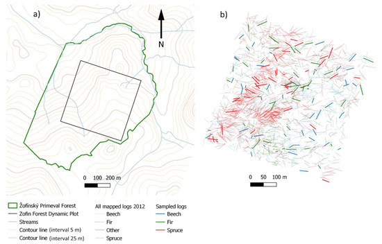
Figure 1.
(a) Location of the Zofin Forest Dynamic Plot within the Žofínský Primeval Forest, contour lines from ČÚZK [36]; (b) Map of downed logs (mapped in 2012) and sampled logs according to tree species.
2.2. Scientific Approach
The basic data set was based on the census from 2012, when a map of trees was created. Based on dendrochronological dating of living trees in the years 2008–2011, a set of logs was selected for sampling. The main parameters for selection were tree species and diameter. This sampling was performed in June 2015 and April 2016. Additional logs were included in the set of sampled logs according to their time of death. Laboratory work was performed immediately after sampling.
The following methods were used to answer the main questions of the study: Changes of relative wood density and moisture per log during decomposition (expressed by TSD and wood density) according to different species have been displayed by statistical models. Decomposition rates were derived from exponential models.
2.3. Tree and Deadwood Censuses
Repeated censuses were carried out in 1975, 1997, 2008 and 2012 in Zofin (25 ha). All standing and downed, live and dead trees and stem fragments of diameter ≥ 10 cm at these sites had been precisely located (Figure 1) and marked with an identification number. Parameters recorded in standing trees were as follows: species, DBH, height, life function (live, dead), character (whole dead tree, broken stem). Standing dead was a tree with height ≥ 1.3 m that was in a position at an angle to the horizontal of more than 45°; only the front of the log was in contact with the ground. Parameters recorded in downed logs included species, decay stage, log position, DBH or bottom diameter, top end diameter, length, and character (whole stem, stem fragment). If a live tree was uprooted by wind in its whole length, the mortality mode was denoted as “windthrow”; the fracture in the basal part at a height below 1.3 m was denoted as “break at stem base”; stem break at a height above 1.3 m created a stem fragment “A”—standing dead tree—and a stem fragment “B”—snap (live stem broken off from the base part) [37]. Log position (binary variable) had been recorded only in 2012. Logs with more than 50% of their length suspended above the ground were included in the category “without ground contact”. Deadwood measurements were carried out according to the so-called Deadwood Protocol [38]. The log or its piece could be in the form of a base part, for which the DBH was measured; or in the form of a fragment of a lying log broken off above breast height, in which the bottom diameter was measured [38]. Each lying log was classified into one of three decay stages as follows. Hard (hereafter “DS 1”): the log still has relatively healthy and hard wood; touchwood (hereafter “DS 2”): there is rot in the core or in the outer mantle of the log, where the wood can be deformed with a blunt object (e.g., a shoe); disintegrated (hereafter “DS 3”): the wood is at a stage of advanced rot, it can be deformed with a blunt object along the entire log, the wood is fragile, and the trunk loses its original shape [38].
2.4. Dating of TSD
To determine the TSD we used a so-called cross-dating technique [35], linking and mutually verifying information from different dendrochronological and tree census data sets. The following 4 approaches were used:
(i) Dendrochronological dating of living trees carried out in 2008–2011 [35]. It included trees that died until 1998. A live tree was cored and its response to disturbance due to the death of adjacent tree was studied in radial growth. Standard dendroecological techniques established by Nowacki and Abrams [39] were linked to the boundary-line approach by Black and Abrams [40]. Positive responses in radial growth ≥ 20% of the boundary line were considered to be a release [41,42]; then, the time since the year of release was assumed to be the TSD of the downed nearby log. If possible, the responses were cross-validated in records of two or three trees in the vicinity of the log. By this approach we decreased the uncertainty of log dating established through repeated censuses to 1–2 years (37 sampled logs). If there was no response greater than 20% or there were several responses above 20% from different years, the sampled log was not considered to be successfully dated. Only release older than 10 years could be detected by dendrochronological dating (until 1998), because the 10-year moving averages were calculated [35].
(ii) The TSD of trees that died and fell until 1998 were estimated as the average TSD of dendrochronologically dated logs of the same species, the same census when a log was first recorded (1975 or 1997) and the same first recorded decay stage (30 sampled logs). It concerned trees that could not be dated by the first method (i). Estimation of the TSD using the same decay stage is not entirely accurate. However, the only other option is to set the TSD as the average year between two censuses (1975 and 1997), and logs that died before 1975 have no maximum time limit.
(iii) The TSD of trees that were killed by the Kyrill storm in January 2007. Freshly fallen trees were marked in the period 2007–2008 soon after the Kyrill windstorm, when they were well recognizable in the forest (27 sampled logs); logs that fell before the Kyrill windstorm were assigned to the middle year between the 1997 census and the 2007 Kyrill event (17 logs).
(iv) The TSD of trees that fell between the 2008 and 2012 censuses were assigned to the middle year between the censuses (15 logs).
Using these dendrochronological data and techniques and repeated tree censuses, we obtained a chronosequence covering 61 years for F. sylvatica decay, 63 years for P. abies decay and 76 years for the decay of A. alba. To determine variability between initial, intermediate, and late decomposition, sampled trees were grouped into three equally long TSD periods (Table 1).

Table 1.
Range of TSD periods.
2.5. Sampling of Downed Deadwood
To select appropriate logs for sampling, we applied the following criteria:
(i) The selection was limited to A. alba, F. sylvatica and P. abies logs. These three main tree species represent 99% of the downed deadwood volume at the research plot.
(ii) Only decaying logs with diameter 45–94 cm were used. By restricting diameter to these intermediate dimensions, we eliminated extreme dimensions significantly affecting the studied decomposition process and large logs that could not be representatively sampled. In total 133 logs (i.e., 42 A. alba, 45 F. sylvatica and 46 P. abies) met these criteria (Table 2). Diameter was measured in the census when the log was first recorded as downed.
Table 2.
Base statistics of sampled downed logs between species. Different letters in Group column indicate significant differences among the species according to mean diameter (one-way ANOVA: F = 1.67, df = 2, p = 0.19, α = 0.05).
(iii) Only those downed logs (stem fragments) that were not recorded as standing deadwood (e.g., fell alive) in former censuses were selected. We are aware that the phase of standing death tree may significantly protract the decomposition rate [8,37]. For downed logs from the 1975 census, it is uncertain whether they fell while alive.
Logs were sampled in different micro-environmental conditions, from the point of view of ground contact (position of the log). Logs of both categories (with and without ground contact) were sampled. Only logs in contact with the ground above approximately 20% of the log length were included in the sampled set, and at the same time at a maximum distance of 1 m from the ground surface. This definition was adopted due to a clear distinction from deadwood in the category of standing dead trees. Lying logs of the following mortality modes were sampled: windthrow, break at stem base, and snap. The location of the sampled logs did not play a role in their selection. The distribution of sampled logs was random on the site (Figure 1). QGIS was used for data visualization [43].
We selected one sample of decomposed wood per downed log from the basal part of the log (at 1.0–1.5 m), at the same time the place of sampling had to meet the condition of the hardest part of the log and the same type of ground contact as the ground contact category of the whole log. So, we consider our results to be the conservative upper limit of the decomposition rate. Samples were collected by an increment corer (inner diameter 12 mm) to a maximum depth of 12 cm, to only sample outer rings (sapwood). The logs were cored from the top side. Bore hole depth was measured by a Vernier calliper, because the pulpy samples could not be reliably measured. The volume of the fresh sample was approximated by a cylinder (π r² h, radius = 6 mm and height equal to the depth of the bore hole) during the calculation. For some decayed logs from which it was not possible to collect a sample with the increment borer, a piece of wood was taken from the disintegrated log, from which a prism was then carved with a hand saw. The volume of the prism was calculated by measuring the length, width, and height. This prism-shaped sample was removed from part of the outer rings when possible, because wood density or other characteristics may differ between the outer and inner parts of decaying logs. Diameter was taken from the census database.
2.6. Laboratory Work
Samples were placed in sealable polypropylene bags and stored in a freezer to prevent the loss of water by evaporation. For analyses, each sample was first weighed to determine the fresh weight, using an analytical laboratory scale (accuracy 0.001 g). Then, drying was carried out at 105 °C for 48 h to a constant weight [7,27], after which samples were again weighed (dried wood sample).
2.7. Calculations
Wood density (g cm−3) is the weight of the dried wood sample divided by the fresh wood sample volume. “Relative wood density” (%) is the wood density divided by density of the dried sample from sound wood (initial density, TSD 0.5 year). Density values of sound wood were taken from freshly fallen and undecomposed logs: 0.411 g cm−3 for A. alba (1 log), 0.558 g cm−3 for F. sylvatica (5 logs), and 0.405 g cm−3 for P. abies (4 logs). “Biomass loss” (%) is 1 minus the proportion of current biomass and initial biomass. Initial biomass is the initial volume of the log multiplied by the density of the sound wood. Current biomass is the current volume of the log multiplied by the wood density. “Density loss” (%) is 1 minus the proportion of wood density and initial density. Gravimetric water content (θg), hereafter “moisture content”, is the weight of water in the wood sample divided by the mass of the dry wood sample expressed in %. “Water content” was calculated as the weight of water in the wood sample divided by the volume of the fresh wood sample (g cm−3).
Log volumes were calculated in PraleStat software [44] as the sum of approximate cone volumes using the DBH (or bottom diameter) and the log length [45]. Current volume is the volume of the log that was measured in the 2012 census. Initial volume (Vi) means the volume of downed log in the year of tree death (1),
where td was the year of tree death, tc was the year of the census when the log was first registered as downed and Vc was the volume of the log measured in this census. The average annual volume loss (AVL) of downed logs for a particular species and diameter of 45–94 cm was calculated as 1 minus the proportion of log volume from two consecutive censuses (e.g., 1975 and 1997). Log volumes from all censuses were used.
Vi = (AVL(tc − td) + 1)Vc
An exponential regression models (2) were generated for relative wood density in relation to TSD (question i) and to estimate the decomposition rate (t0.95) and half-life (t0.5) for downed logs belonging to particular species (question iii),
where for the question (iii) the explanatory variable was the TSD of downed logs and the response variable was the biomass (or density) loss of the logs. The decomposition rate and half-life were used to compare density loss and biomass loss. The lm () function was used to fit the exponential regression model in R software [46] using the natural log of response variable (y): lm(log(y)~ x). 95% confidence intervals were modelled by the following example of function in R software: exp (predict (exp.beech, newdata = data.frame (TSD = seq (4, 120, by = 0.1)), interval = “confidence”, level = 0.95)), where “exp.beech” is the exponential regression model for F. sylvatica.
y = abx
Assuming a commonly used single negative exponential decay model, a decomposition rate constant k (year−1) was also calculated for each sampled log, and used to derive decomposition rates and half-lives as the mean value for each species according to equations from Olson [17]:
where X is the current biomass (or density), X0 is the initial biomass (or density) and t is TSD.
k = −ln(X/X0)/t
t0.95 = −ln(0.05)/k = 2.996/k
t0.5 = −ln(0.5)/k = 0.693/k
Mean values of wood density and water content for decay stages were calculated. To estimate biomass and water storage of downed deadwood per hectare (Mg ha−1), values of the volume of downed deadwood from the 2012 census were taken into account. Confidence intervals (CI) were calculated according to Equation (6),
where is sample mean, z is confidence level value, s is sample standard deviation and n is sample size. The critical level of significance was α = 0.05. Water storage of other species (Acer pseudoplatanus L., Ulmus glabra Huds; representation in downed deadwood is 1%) were calculated as for F. sylvatica. Biomass and water storage in the plot are shown in Appendix A.
2.8. Statistical Tests
The assumptions of normality for relative wood density (question i), density loss and biomass loss (question iii) within each species were tested by the Anderson–Darling test.
Differences between the two types of log positions were tested for log moisture. The logs were divided according to the tree species and decay stages. The assumptions of normality were tested by the Anderson–Darling test, and homogeneity of variances by Bartlett test. For data with normal distribution, two sample t-test was used for data with homogeneous variance or Welch two sample t-test for data with unequal variances. The Mann–Whitney U test was used for data with non-normal distribution.
Changes in moisture during decomposition are expressed by linear regression—especially by the parameter b (slope). The degree of linear dependence between density (explanatory variable) and moisture content (response variable) was obtained using Pearson´s correlation coefficient (r). Variability is expressed by the interquartile range and standard deviation. Additionally for question (iii), the assumptions of normality and homogeneity of variances were tested.
Since samples of F. sylvatica and P. abies were collected in June 2015, while samples of A. alba were collected in April 2016, the moisture of A. alba was not compared with that of F. sylvatica and P. abies. There was uncertainty as to how much the climate in different seasons (spring and summer) could affect the moisture of the downed deadwood. A weak correlation was found between instantaneous CWD moisture and initial moisture, duration and amount of precipitation, and average temperature [47,48]. Responsible factors probably included wind conditions or vapor condensation [47]. The effect of precipitation and temperature on the downed deadwood moisture under fixed site conditions has not yet been studied. Mean monthly precipitation and temperature for the period 2017–2020 in Zofin can be found in Appendix A.
All calculations, analysis, models and graph creation were performed in the R software [46]. Statistical significance was considered at the level of α = 0.05.
3. Results
3.1. Changes in Relative Wood Density during the Decomposition Process
Changes in the relative wood density during TSD are shown in Figure 2 as exponential regression model. Values of relative wood density were normally distributed according to the Anderson–Darling test for all tree species. Although the exponential model was statistically significant for F. sylvatica and P. abies, it was not significant for A. alba. Spruce showed the highest R-squared (R2 = 0.299). Although F. sylvatica and P. abies logs had a decreasing change in relative wood density during TSD according to the regression model, the values of relative wood density of A. alba logs practically did not change during TSD.
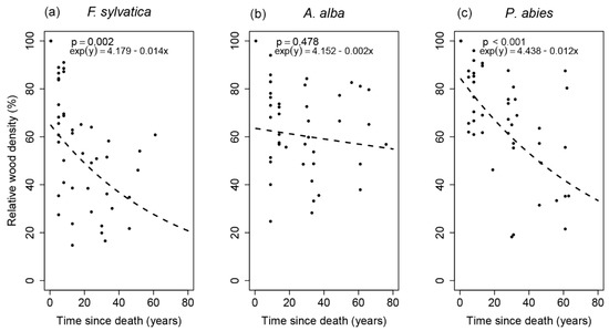
Figure 2.
Exponential regression models between the relative wood density and time since death.
Variability in the relative wood density of F. sylvatica logs peaked in TSD period 1 and then decreased to TSD period 3, when the lowest variability in terms of interquartile range was found (Table 3). In contrast, the relative wood density variability of A. alba logs increased with increasing TSD; the highest interquartile range was found in TSD period 3. Variability in the relative wood density of P. abies logs approximately increased with increasing TSD; the highest interquartile range was found in TSD period 3 (Table 2).
Table 3.
Interquartile ranges of relative wood density and moisture content over periods of TSD.
3.2. Effect of Variables on Changes in Moisture Content
Variability in the moisture content were the highest in TSD period 2 for A. alba and F. sylvatica, while for P. abies it was the highest in TSD period 3 (Table 3).
Changes in the deadwood moisture content over TSD were expressed by linear regressions that were statistically significant for A. alba, F. sylvatica and P. abies (Figure 3). The models showed increasing linear relationships, with F. sylvatica showing the highest R-squared (R2 = 0.276). The rate of change (slope) of moisture content with TSD was the highest for F. sylvatica (bF.sylvatica = 3.94) and lower for the coniferous species (bA.alba = 2.21, bP.abies = 1.93).
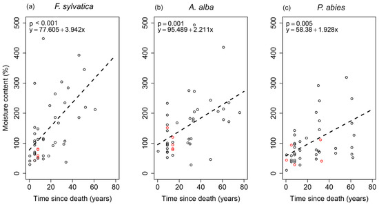
Figure 3.
Linear regression models between the moisture content and time since death for each tree species: (a) F. sylvatica; (b) A. alba; (c) P. abies. Red circles—logs without ground contact.
The degree of linear dependence between the wood density and moisture content (Pearson´s correlation coefficient r) is shown in Figure 4. These variables showed decreasing linear relationships, and F. sylvatica again had the highest R-squared (R2 = 0.390). Although F. sylvatica deadwood showed a strong negative relationship between the wood density and moisture content (r = −0.62), A. alba and P. abies deadwood showed moderate negative relationships (r = −0.45 and r = −0.46). The deadwood moisture of the three tree species was measured, and F. sylvatica and P. abies were compared as the two species were sampled at the same time. However, values of moisture were not significantly different between F. sylvatica and P. abies for any of the TSD periods. The effects of wood density and diameter on moisture and water content were analyzed in Appendix A.

Figure 4.
Correlation between the moisture content and wood density for each tree species: (a) F. sylvatica; (b) A. alba; (c) P. abies. Red circles—logs without ground contact.
Regarding the position of the log, 13.3% of A. alba, 24.5% of F. sylvatica, and 43.7% of P. abies logs from downed deadwood at the research plot were without ground contact. A total of 20.8% of A. alba, 16.1% of F. sylvatica, and 45.9% of P. abies from the sampled logs were without ground contact. Moisture content differences for logs with and without ground contact in the same decay stage and tree species were tested; however only DS 1 and 2 were included because all DS 3 logs in the sampled set were with ground contact (in Zofin overall, only 3.3% of the downed logs in DS 3 were without ground contact). For F. sylvatica and P. abies, no significant differences in terms of moisture content were found between logs with and without ground contact (p values from 0.138 to 0.492). However, for A. alba, significant differences were found between logs with and without ground contact (pDS1 = 0.019, pDS2 = 0.004). The average moisture content for A. alba logs in DS 1 without ground contact was 77.3%, while for logs with ground contact was 142.0%. In DS 2, the moisture content was 94.6% and 150.6% for A. alba logs without and with ground contact. The proportions of water storage for tree species and decay stages are given in Appendix A.
3.3. The Decomposition Ratees of Downed Logs
Values of the half-life and decomposition rate for downed logs with diameter 45–94 cm are shown in Table 4, and exponential models are shown in Figure 5. Although values of density and biomass loss for A. alba and F. sylvatica were normally distributed according to the Anderson–Darling test, values of P. abies density and biomass loss were not.
Table 4.
Estimated decomposition rates and half-lives (years) and their 95% confidence intervals in parentheses, decomposition rate constants k (year−1) and values of models fit.
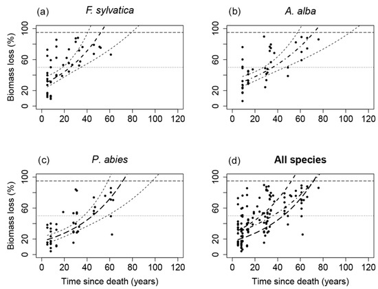
Figure 5.
Exponential models of the decomposition rate and half-life based on the biomass loss of downed logs for each tree species (a) F. sylvatica; (b) A. alba; (c) P. abies. (d) Logs of all tree species together with the line type according to the tree species: dashed line—F. sylvatica; dash-dotted line—A. alba; long-dashed line—P. abies.
Differences in the decomposition rate constant k and derived decomposition rates based on density loss vs. biomass loss were highest for A. alba (∆ k = 0.08, ∆ t0.95 = 23 years), and lower for F. sylvatica (∆ k = 0.03, ∆ t0.95 = 4 years) and P. abies (∆ k = 0.03, ∆ t0.95 = 13 years). Exponential model fit values were significantly better for biomass loss, especially for A. alba where the model of density loss was not statistically significant (Table 4). The better model fit for biomass loss also resulted in narrower 95% confidence intervals, i.e., more accurate estimates of decomposition rates (t0.95). The confidence intervals for F. sylvatica and P. abies t0.95 based on biomass loss were 38 and 39 years, while for density loss were 98 and 111 years. The effect of moisture content on the decomposition rates are shown in Appendix A.
4. Discussion
4.1. Changes in Relative Wood Density and Moisture during the Decomposition Process
We described trajectories of deadwood moisture increases and density decreases during the decomposition of downed logs. Mackensen and Bauhus [15] observed similar trends of moisture within TSD classes in south-eastern Australia, with moisture content increasing with age until 12 years of TSD for one species of Pinus and two species of Eucalyptus. In a study on spruce and larch deadwood on Cambisols, Umbrisols, and Podzols in a mountain forest, Petrillo et al. [26] concluded that an increasing water content and decreasing density of deadwood during the decomposition process could be explained by the gradual loss of wood structure (as in our relationship in Figure 4). Similar results have also been found in other studies on F. sylvatica [10] and P. abies deadwood [27]. In contrast, studying five mountain sites with A. alba, F. sylvatica and P. abies logs, Pichler et al. [48] found on that the moisture of F. sylvatica deadwood reached maximum values in decay stage 2 and moisture decreased in decay stage 3, while the moisture of P. abies deadwood reached minimum values in decay stage 2 (showing a U-shaped distribution). In another study, Paletto and Tossi [13] similarly observed moisture content decreasing from the first decay stage to the third decay stage, after which it increased rapidly to the fifth decay stage in subalpine and mountainous P. abies, mountainous mixed P. abies—A. alba and submountainous F. sylvatica forests.
We found that the dependence of wood moisture on the TSD and density was different between deciduous and coniferous species, being more significant in F. sylvatica than in A. alba and P. abies (Figure 3 and Figure 4). In addition, the proportion of the variance (R2) for moisture that is explained by the TSD and density is higher in downed F. sylvatica logs. Other unmeasured factors probably have greater effects on the moisture contents of A. alba and P. abies wood. Downed deadwood significantly increases water storage in a forest ecosystem. Late-decay deadwood has a higher moisture-holding capacity compared to topsoil, and may thus be used as refugia for small mammals, salamanders and soil-inhabiting organisms during hot and dry seasons [49,50,51].
The variability in moisture content could not be largely explained by differences in soil properties and the different exposure of logs to sunlight. All sampled logs were located on well-drained acidic soils and under the tree canopy. The high variability in relative wood density could have been caused by the colonization of different species of fungi and bacteria. The high number of macrofungal species in Zofin (known 800 species [52]) and the considerable differences in decomposer communities between individual logs [3] may have contributed to the wider interval of decomposition rates.
4.2. Decomposition Rates of Downed Logs
Downed logs at the same site decomposing for the same amount of time showed highly divergent values of density and biomass loss (Figure 5). The rate of downed deadwood decomposition was strongly different among logs. This was most likely due to properties of the wood substrate and environmental conditions. Downed logs differed in their mode and cause of mortality—treethrows or breakages, competition, or senescence. Each mortality mode can undergo different decomposition pathways by different decomposers, thus affecting the decomposition rate [53]. There are an unknown proportion of trees in which heartwood start decaying already during the life of the tree (typical for senescent trees). The existence of decaying wood in living trees is an important factor that shortens the residence time after such trees fall. We restricted our choice of downed logs to intermediate diameter to avoid bias from decomposition in extreme size categories; however, even the different diameters of the downed logs we studied (diameter 45–94 cm) certainly affect the decomposition rate. Micro-environmental conditions (temperature, water availability and gaseous regime) could have also played a role, and likely influenced the composition of saproxylic fungi communities and respirational carbon loss [54]. Herrmann et al. [8] also observed high variation in deadwood density within decay stages and hence only a few significant differences between adjacent decay stages within a given species. Our study did not aim to test the various factors influencing the different decay times of individual downed logs, but we rather intended to describe decomposition using the most homogeneous set of sampled logs available.
Krüger et al. [55] determined decomposition rate of downed F. sylvatica logs by radiocarbon dating to be 24 years in a beech-oak forest, and 35 years was reported in a beech forest on podsolic brown earth soil [19]. A decomposition rate of 54 years was reported from 4 sites on Luvisols, Cambisols, and Podsolic Cambisols by Herrmann et al. [8]. Kraigher et al. [10] modelled the decomposition rate of decaying F. sylvatica logs as 51 years in two fir-beech forests on Eutric Cambisols and Rendzic Leptosols. Finally, in two studies examining the trajectory of downed deadwood from natural temperate forests in Central Europe [37,56], decomposition rates were 43 and 57 years for F. sylvatica and A. alba logs of diameter 55+ cm at the same site (Zofin). For comparison, the decomposition rates based on biomass loss were 50 and 52 years for F. sylvatica and 71 and 83 years for A. alba, respectively, according to the different models presented here (Table 4). These are therefore longer decomposition rates than in previous studies at Zofin [37,56]. One factor leading to these differences is the fact that the decomposition rates here were calculated only from those logs that remain to the present, i.e., those with the slowest decay rate. In contrast, decomposition rates in the previous studies were calculated from all logs, even those that are currently completely decomposed. Another difference is in the models used—survival function vs. exponential.
Holeksa et al. [9] found that the decomposition rate of decaying P. abies wood was 71–113 years, with higher values for thicker stems on Skeletic Podzols and Humic–Albic Umbrisols and Dystric-Stagnic Cambrisols. Herrmann et al. [8] deduced from 5 sites on Luvisols, Cambisols, and Podsolic Cambisols that the decomposition rate was 88 years. Petrillo et al. [57] calculated residence times of P. abies deadwood to 45, 56, and 84 years based on different methods on Cambisols, Umbrisols, and Podzols. Using the different approaches in our study, we found decomposition rates based on biomass loss for P. abies of 72 and 109 years.
The different residence times of lying decaying logs also have effects on underlying forest soils that are dependent on the tree species. During beech log decay, underlying Entic Podzols have been shown to responded with a significant increase of nutrients, pH, and effective cation exchange capacity, and the maximal divergence compared to control sites was reached between 12 and 60 years after the trunk fell [58]. The even longer decay of coniferous deadwood could have an even longer lasting effect on soils.
5. Conclusions
Although sound beech wood had a higher density (0.558 g cm−3) than spruce and fir wood (0.405–0.411 g cm−3), it was subject to faster degradation in the initial phase of decomposition. Our study shows that tree species and time since death are key factors influencing the amount of water in deadwood. There was 217–517 kg of water per m3 in the downed deadwood, depending on the tree species and decay stage, which increases the water storage capacity of the forest ecosystem and provides resources for organisms, especially during dry seasons. Although logs were selected to have very similar climatic conditions in terms of altitude, tree canopy, and soil water regime, the variability of moisture of wood was quite high and varied with TSD, with the highest variability found in intermediate TSD period for A. alba and F. sylvatica, while for P. abies in late TSD period. Downed logs had considerable variability in their relative wood density during decomposition. Deadwood moisture was affected by the seasonality of the climate, so it would be necessary to take samples several times a year for more accurate moisture values for evaluations of deadwood retention capacity. The results of this study can be used to predict deadwood dynamics in terms of biomass, water storage, and subsequent changes in biodiversity, to formulate management recommendations, as well as to assess spatial soil complexity and patterns of biogeomorphic processes.
Author Contributions
Conceptualization, T.P.; methodology, T.P. and P.Š.; validation, T.P.; formal analysis, T.P.; investigation, T.P. and P.Š.; resources, T.P.; data curation, T.P. and P.Š.; writing—original draft preparation, T.P.; writing—review and editing, T.P. and P.Š.; visualization, T.P.; supervision, T.P.; project administration, T.P. and P.Š.; funding acquisition, T.P. and P.Š. All authors have read and agreed to the published version of the manuscript.
Funding
This research was funded by Grantová Agentura České Republiky, grant number 19-09427S and the student Interní grantová agentura Mendelovy univerzity v Brně, grant no. 6/2015 “Deadwood density variation with time since death of Picea abies and Fagus sylvatica”.
Institutional Review Board Statement
Not applicable.
Informed Consent Statement
Not applicable.
Data Availability Statement
Not applicable.
Acknowledgments
We would like to thank our colleagues Dušan Adam and Libor Hort for managing the tree census databases 1975–2012, the Department of Wood Science in Mendel University in Brno for facilitating the laboratory analysis, and David Hardekopf for English proofreading.
Conflicts of Interest
The authors declare no conflict of interest.
Appendix A
Appendix A.1. Downed Deadwood Biomass and Water Storage in the Plot
During the 2012 census in Zofin, the following total amounts of dry biomass in downed deadwood were recorded (with confidence intervals): 27.4 (23.7–31.0) Mg.ha−1 in F. sylvatica logs, 16.6 (14.4–18.8) Mg ha−1 in A. alba logs, 43.8 (39.9–47.7) Mg ha−1 in P. abies logs and 0.6 (0.5–0.7) Mg ha−1 in logs of other species; in total 88.4 (76.8–99.8) Mg ha−1. The volume of deadwood represented a significant proportion of the aboveground wood volume in the 2012 census, with downed deadwood comprising 32.6% of the aboveground wood volume, and standing deadwood comprising 12.2% of the aboveground volume. The volume of deadwood was higher than the volume of living wood in A. alba and P. abies. In F. sylvatica, on the other hand, this ratio was reversed (Figure A1). The distribution of deadwood biomass and water mass by species and decay stages is shown in Figure A2. There was an unbalanced structure of decay stages mainly for F. sylvatica and P. abies deadwood, caused by the disturbance event in 2007. The dry biomass in downed deadwood resulting from this exceptional disturbance event was 35.1 Mg ha−1 in 2012, which is a 72.9% increase compared to the 1997 census before the windstorm, when the dry biomass in downed deadwood was 48.2 Mg ha−1. It must be taken into account that logs that fell during this disturbance belonging to DS 1 (the highest wood density) represented 95.9% of the volume of logs falling during this windstorm.
The water storage was 29.3 (22.9–35.6) Mg ha−1 in downed F. sylvatica logs and 35.5 (26.4–44.5) Mg ha−1 in downed P. abies logs in the summer, 24.9 (19.7–30.0) Mg ha−1 in downed A. alba logs in the spring, and 0.6 (0.51–0.75) Mg ha−1 in downed logs of other species; in total approximately 87.8 (64.6–111.1) Mg ha−1.
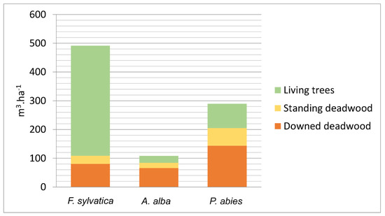
Figure A1.
Volume of living trees and deadwood per tree species in Zofin according to the 2012 census.
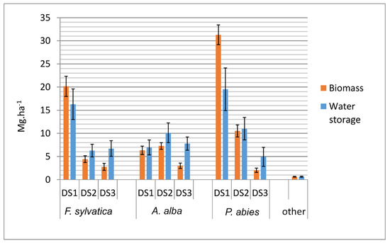
Figure A2.
Amounts of biomass and water storage in downed deadwood according to species and decay stage in Zofin. Error bars display confidence intervals.
Appendix A.2. The Effect of Wood Density and Diameter on Moisture and Water Content
A total of 56 sampled F. sylvatica logs of diameter 35–100 cm was used in the analysis. This dataset was divided into 2 groups with equal numbers of logs. Smaller size logs had diameter 35–64 cm, larger sized logs had diameter 65–100 cm. The rate of change (slope) of moisture content with TSD was higher for larger sized logs (b = 5.38) than for smaller sized logs (b = 1.73). Smaller sized logs had average TSD 15 years and average moisture content 129%, larger sized logs had average TSD 19 years and average moisture content 164%.
The dataset of F. sylvatica logs was then divided into 2 groups depending on wood density. Lower density logs had values 0.082–0.302 g.cm−3, higher density logs had values 0.313–0.711 g.cm−3. The rate of change of moisture content with TSD was higher for lower density logs (b = 3.13) than for higher density logs (b = 1.87).
A total of 53 sampled A. alba logs of diameter 40–110 cm and 61 sampled P. abies logs of diameter 35–110 cm was divided into 2 groups with equal numbers of logs. Mean values of water content (g.cm−3) did not indicate a visible effect of diameter (expressed by diameter category) on the amount of water in the downed deadwood (Table A1).
Table A1.
Mean values of water content (kg.m−3) depending on decay stage, species, and diameter of downed logs.
Table A1.
Mean values of water content (kg.m−3) depending on decay stage, species, and diameter of downed logs.
| F. sylvatica | A. alba | P. abies | ||||
|---|---|---|---|---|---|---|
| Decay Stage | Diameter | Diameter | Diameter | |||
| 35–64 cm | 65–100 cm | 40–70 cm | 71–110 cm | 35–60 cm | 61–110 cm | |
| DS 1 | 332.2 | 350.0 | 236.2 | 367.1 | 224.4 | 186.8 |
| DS 2 | 339.9 | 308.8 | 371.9 | 339.7 | 259.1 | 294.1 |
| DS 3 | 540.3 | 503.7 | 467.6 | 503.5 | 469.7 | 445.8 |
Appendix A.3. The Effect of Moisture Content on the Decomposition Rates
A total of 133 sampled logs of diameter 45–94 cm was divided into 2 groups with equal numbers of logs according to moisture content for each species. The decomposition rates derived from the decomposition rate constant k based on biomass loss were calculated. F. sylvatica logs with lower moisture content (29–103%) had the decomposition rate 72 years, while logs with higher moisture content (107–542%) had the decomposition rate 45 years. A. alba logs with different moisture content category had the same decomposition rates (89 years). P. abies logs with lower moisture content (10–76%) had the decomposition rate 130 years, while logs with higher moisture content (78–543%) had the decomposition rate 111 years. Although these results indicated a longer decomposition rate for logs with lower moisture (F. sylvatica and P. abies), these logs had a lower average TSD (moisture content dependence on TSD in Figure 2). As it turned out, the decay rate constant k is higher in logs in initial decay phase (lower TSD).
Appendix A.4. Diameter Distribution of Logs
Table A2.
Diameter distribution of the sampled logs used for analyzes. Diameter classes are diameters of logs rounded to the nearest tens.
Table A2.
Diameter distribution of the sampled logs used for analyzes. Diameter classes are diameters of logs rounded to the nearest tens.
| Diameter Class (cm) | Total | |||||
|---|---|---|---|---|---|---|
| 50 | 60 | 70 | 80 | 90 | ||
| Number of logs | 25 | 24 | 35 | 26 | 23 | 133 |
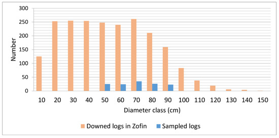
Figure A3.
Diameter structure of downed deadwood in Zofin (25 ha) and sampled logs. Diameter classes are diameters of logs rounded to the nearest tens.
Appendix A.5. Climate Data
Aridity index has been calculated according the following equation [59,60]:
where Pm is monthly precipitation [mm] and Tm is mean monthly temperature [°C]. Higher values of the aridity index indicate a more humid climate. Climate data from Zofin showed considerable differences in values of aridity index between months when taking into account April and June with their previous months mainly in the period 2018–2020. Data from the period 2015–2016 were not available. Therefore, these data only serve to illustrate the fluctuation of values during sampling period
IDM = 12Pm/(Tm + 10)
Table A3.
Mean monthly temperatures (Tm), mean monthly precipitation (Pm) and aridity indexes (IDM) in the months of sampling (April, June) and in the previous month from period 2017–2020. Data were obtained from the field climatic station in Zofin.
Table A3.
Mean monthly temperatures (Tm), mean monthly precipitation (Pm) and aridity indexes (IDM) in the months of sampling (April, June) and in the previous month from period 2017–2020. Data were obtained from the field climatic station in Zofin.
| Month, Year | Tm | Pm | IDM |
|---|---|---|---|
| March 2017 | 4.31 | 49.20 | 41.26 |
| April 2017 | 4.79 | 108.00 | 87.60 |
| May 2017 | 11.86 | 75.20 | 41.27 |
| June 2017 | 16.42 | 62.40 | 28.35 |
| March 2018 | −0.75 | 35.00 | 45.42 |
| April 2018 | 11.40 | 15.40 | 8.64 |
| May 2018 | 13.61 | 94.00 | 47.79 |
| June 2018 | 15.04 | 166.40 | 79.74 |
| March 2019 | 4.96 | 7.40 | 5.93 |
| April 2019 | 7.41 | 27.60 | 19.02 |
| May 2019 | 8.08 | 149.80 | 99.41 |
| June 2019 | 18.67 | 90.80 | 38.00 |
| March 2020 | 2.27 | 35.80 | 35.00 |
| April 2020 | 7.81 | 24.20 | 16.30 |
| May 2020 | 8.98 | 113.00 | 71.44 |
| June 2020 | 13.93 | 232.40 | 116.56 |
References
- Ódor, P.; Hees, A.F.M. Preferences of dead wood inhabiting bryophytes for decay stage, log size and habitat types in Hungarian beech forests. J. Bryol. 2004, 26, 79–95. [Google Scholar] [CrossRef]
- Savely, H.E., Jr. Ecological relations of certain animals in dead pine and oak logs. Ecol. Monogr. 1939, 9, 322–385. [Google Scholar] [CrossRef]
- Baldrian, P.; Zrůstová, P.; Tláskal, V.; Davidová, A.; Merhautová, V.; Vrška, T. Fungi associated with decomposing deadwood in a natural beech-dominated forest. Fungal Ecol. 2016, 23, 109–122. [Google Scholar] [CrossRef]
- Rajala, T.; Peltoniemi, M.; Pennanen, T.; Mäkipää, R. Fungal community dynamics in relation to substrate quality of decaying Norway spruce (Picea abies [L.] Karst.) logs in boreal forests. FEMS Microbiol. Ecol. 2012, 81, 494–505. [Google Scholar] [CrossRef] [Green Version]
- Cornwell, W.K.; Cornelissen, J.H.C.; Allison, S.D.; Bauhus, J.; Eggleton, P.; Preston, C.M.; Scarff, F.; Weedon, J.T.; Wirth, C.; Zanne, A.E. Plant traits and wood fates across the globe: Rotted, burned or consumed? Glob. Chang. Biol. 2009, 15, 2431–2449. [Google Scholar] [CrossRef] [Green Version]
- Šamonil, P.; Daněk, P.; Senecká, A.; Adam, D.; Phillips, J.D. The biomechanical effects of trees in a temperate forest. Earth Surf. Proc. Land 2018, 43, 1063–1072. [Google Scholar] [CrossRef]
- Müller-Using, S.; Bartsch, N. Decay dynamic of coarse and fine woody debris of beech (Fagus sylvatica L.) forest in Central Germany. Eur. J. For. Res. 2009, 128, 287–296. [Google Scholar] [CrossRef] [Green Version]
- Herrmann, S.; Kahl, T.; Bauhus, J. Decomposition dynamics of coarse woody debris of three important central European tree species. For. Ecosyst. 2015, 2, 27. [Google Scholar] [CrossRef] [Green Version]
- Holeksa, J.; Zielonka, T.; Żywiec, M. Modelling the decay of coarse woody debris in a subalpine Norway spruce forest of the West Carpathians, Poland. Can. J. For. Res. 2008, 38, 415–428. [Google Scholar] [CrossRef]
- Kraigher, H.; Jurc, D.; Kalan, P.; Kutnar, L.; Levanic, T.; Rupel, M.; Smolej, I. Beech Coarse Woody Debris Characteristics in two Virgin Forest Reserves in Southern Slovenia. Zb. Gozdarstva Lesar. 2002, 69, 91–134. [Google Scholar]
- Lombardi, F.; Cherubini, P.; Lasserre, B.; Tognetti, R.; Marchetti, M. Tree rings used to assess time since death of deadwood of different decay classes in beech and silver fir forests in the central Apenines (Molise, Italy). Can. J. For. Res. 2008, 38, 821–833. [Google Scholar] [CrossRef]
- Lombardi, F.; Cherubini, P.; Tognetti, R.; Cocozza, C.; Lasserre, B.; Marchetti, M. Investigating biochemical processes to assess deadwood decay of beech and silver fir in Mediterranean mountain forests. Ann. For. Sci. 2013, 70, 101–111. [Google Scholar] [CrossRef] [Green Version]
- Paletto, A.; Tossi, V. Deadwood density variation with decay class in seven tree species of the Italian Alps. Scand. J. For. Res. 2010, 25, 164–173. [Google Scholar] [CrossRef]
- Krankina, O.N.; Harmon, M.E. Dynamics of the dead wood carbon pool in northwestern Russian boreal forests. Water Air Soil Poll. 1995, 82, 227–238. [Google Scholar] [CrossRef]
- Mackensen, J.; Bauhus, J. Density loss and respiration rates in coarse woody debris of Pinus radiate, Eucalyptus regnans and Eucalyptus maculate. Soil Biol. Biochem. 2003, 35, 177–186. [Google Scholar] [CrossRef]
- Harmon, M.E.; Franklin, J.F.; Swanson, F.J.; Sollins, P.; Gregory, S.V.; Lattin, J.D.; Anderson, N.H.; Cline, S.P.; Aumen, N.G.; Sedell, J.R.; et al. Ecology of Coarse Woody Debris in Temperate Ecosystem. Adv. Ecol. Res. 1986, 15, 133–302. [Google Scholar] [CrossRef]
- Freschet, G.T.; Weedon, J.T.; Aerts, R.; van Hal, J.R.; Cornelissen, J.H.C. Interspecific differences in wood decay rates: Insights from a new short-term method to study long-term wood decomposition. J. Ecol. 2012, 100, 161–170. [Google Scholar] [CrossRef]
- Graham, R.L.; Cromack, J.R.K. Mass, nutrient content, and decay rate of dead boles in rain forests of Olympic National Park. Can. J. For. Res. 1982, 12, 511–522. [Google Scholar] [CrossRef]
- Shorohova, E.; Kapitsa, E. Influence of the substrate and ecosystem attributes on the decomposition rates of coarse woody debris in European boreal forests. For. Ecol. Manag. 2014, 315, 173–184. [Google Scholar] [CrossRef]
- Næsset, E. Decomposition rate constants of Picea abies logs in southeastern Norway. Can. J. For. Res. 1999, 29, 372–381. [Google Scholar] [CrossRef]
- Boddy, L. Fungal community ecology and wood decomposition processes in angiosperms: From standing tree to complete decay of coarse woody debris. Ecol. Bull. 2001, 49, 43–56. [Google Scholar]
- Olson, J.S. Energy storage and the balance of producers and decomposers in ecological systems. Ecology 1963, 44, 322–331. [Google Scholar] [CrossRef] [Green Version]
- Minderman, G. Addition, decomposition and accumulation of organic matter in forests. J. Ecol. 1968, 56, 355–362. [Google Scholar] [CrossRef]
- Zell, J.; Kändler, G.; Hanewinkel, M. Predicting constant decay rates of coarse woody debris–a meta-analysis approach with a mixed model. Ecol. Model. 2009, 220, 904–912. [Google Scholar] [CrossRef]
- Bütler, R.; Patty, L.; Le Bayon, R.-C.; Guenat, C.; Schlaepfer, R. Log decay of Picea abies in the Swiss Jura Mountains of central Europe. For. Ecol. Manag. 2007, 242, 791–799. [Google Scholar] [CrossRef] [Green Version]
- Petrillo, M.; Cherubini, P.; Sartori, G.; Abiven, S.; Ascher, J.; Bertoldi, D.; Camin, F.; Barbero, A.; Larcher, R.; Egli, M. Decomposition of Norway spruce and European larch coarse woody debris (CWD) in relation to different elevation and exposure in an Alpine setting. iForest 2015, 9, 154–164. [Google Scholar] [CrossRef] [Green Version]
- Teodosiu, M.; Bouriaud, O.B. Deadwood specific density and its influential factors: A case study from a pure Norway spruce old-growth forest in the Eastern Carpathians. For. Ecol. Manag. 2012, 283, 77–85. [Google Scholar] [CrossRef]
- Hoppe, B.; Purahong, W.; Wubet, T.; Kahl, T.; Bauhus, J.; Arnstadt, T.; Hofrichter, M.; Buscot, F.; Krüger, D. Linking molecular deadwood-inhabiting fungal diversity and community dynamics to ecosystem functions and processes in Central European forests. Fungal Divers. 2015, 77, 367–379. [Google Scholar] [CrossRef]
- Kubartová, A.; Ottosson, E.; Dahlberg, A.; Stenlid, J. Patterns of fungal communities among and within decaying logs revealed by 454 sequencing. Mol. Ecol. 2012, 21, 4514–4532. [Google Scholar] [CrossRef] [PubMed]
- Průša, E. Die Bomischen und Mahrischen Urwalder—Ihre Struktur und Okologie; Academia Verlag: Praha, Czech Republic, 1985. [Google Scholar]
- Michéli, E.; Schad, P.; Spaargaren, O.; Dent, D.; Nachtergale, F. World Reference Base for Soil Resources; World Soil Resources Reports; Food and Agricultural Organization of the United Nations: Rome, Italy, 2006; Volume 103. [Google Scholar]
- Šamonil, P.; Valtera, M.; Bek, S.; Šebková, B.; Vrška, T.; Houška, J. Soil variability through spatial scales in a permanently disturbed natural spruce-fir-beech forest. Eur. J. For. Res. 2011, 130, 1075–1091. [Google Scholar] [CrossRef]
- Tolasz, R.; Míková, T.; Valeriánová, A.; Voženílek, V. Atlas Podnebí Česka; Univerzita Palackého v Olomouci—ČHMU: Olomouc, Czech Rebublic, 2007. [Google Scholar]
- Janík, D.; Král, K.; Adam, D.; Hort, L.; Šamonil, P.; Unar, P.; Vrška, T.; McMahon, S. Tree spatial patterns of Fagus sylvatica expansion over 37 years. For. Ecol. Manag. 2016, 375, 134–145. [Google Scholar] [CrossRef] [Green Version]
- Šamonil, P.; Doleželová, P.; Vašíčková, I.; Adam, D.; Valtera, M.; Král, K.; Janík, D.; Šebková, B. Individual-based approach to the detection of disturbance history through spatial scales in a natural beech-dominated forest. J. Veg. Sci. 2013, 24, 1167–1184. [Google Scholar] [CrossRef]
- Český Úřad Zeměměřický a Katastrální—ČÚZK. Základní Báze Geografických dat České Republiky (ZABAGED®), Výškopis–grid 10 × 10 m. Available online: https://ags.cuzk.cz/geoprohlizec/?m=META_ZBG_GRID10 (accessed on 1 January 2014).
- Přívětivý, T.; Janík, D.; Unar, P.; Adam, D.; Král, K.; Vrška, T. How do environmental conditions affect the deadwood decomposition of European beech (Fagus sylvatica L.)? For. Ecol. Manag. 2016, 381, 177–187. [Google Scholar] [CrossRef]
- Král, K.; Valtera, M.; Janík, D.; Šamonil, P.; Vrška, T. Spatial variability of general stand characteristics in central European beech-dominated natural stands—Effects of scale. For. Ecol. Manag. 2014, 328, 353–364. [Google Scholar] [CrossRef]
- Nowacki, G.J.; Abrams, M.D. Radial-growth averaging criteria for reconstructing disturbance histories from presettlement-origin oaks. Ecol. Monogr. 1997, 67, 225–249. [Google Scholar] [CrossRef]
- Black, B.A.; Abrams, M.D. Use boundary-line growth patterns as a basis for dendroecological release criteria. Ecol. Appl. 2003, 13, 1733–1749. [Google Scholar] [CrossRef] [Green Version]
- Šamonil, P.; Schaetzl, R.J.; Valtera, M.; Goliáš, V.; Baldrian, P.; Vašíčková, I.; Adam, D.; Janík, D.; Hort, L. Crossdating of disturbances by tree uprooting: Can treethrow microtopography persist for 6000 years? For. Ecol. Manag. 2013, 307, 123–135. [Google Scholar] [CrossRef]
- Vašíčková, I.; Šamonil, P.; Fuentes, U.A.E.; Král, K.; Daněk, P.; Adam, D. The true response of Fagus sylvatica L. to disturbances: A basis for the empirical inference of release criteria for temperate forests. For. Ecol. Manag. 2016, 374, 174–185. [Google Scholar] [CrossRef]
- QGIS.org. QGIS Geographic Information System. QGIS Association. Available online: http://www.qgis.org (accessed on 1 June 2021).
- Pralesy ČR. PraleStat Software. Available online: https://naturalforests.cz/research-pralestat-software#v4 (accessed on 1 June 2021).
- Petráš, R. Matematický model tvaru kmeňa listnatých drevín. Lesn. Cas. 1990, 36, 231–241. [Google Scholar]
- R Core Team. R: A Language and Environment for Statistical Computing; R Foundation for Statistical Computing: Vienna, Austria, 2021; Available online: http://www.R-project.org (accessed on 14 May 2021).
- Brackebusch, A.P. Gain and Loss of Moisture in Large Forest Fuels; USDA Forest Service: Ogden, UT, USA, 1975. [Google Scholar]
- Pichler, V.; Homolák, M.; Skierucha, W.; Pichlerová, M.; Ramírez, D.; Gregor, J.; Jaloviar, P. Variability of moisture in coarse woody debris from several ecologically important tree species of the Temperate Zone of Europe. Ecohydrology 2012, 5, 424–434. [Google Scholar] [CrossRef]
- Fauteux, D.; Mazerolle, M.J.; Imbeau, L.; Drapeau, P. Site occupancy and spatial co-occurence of boreal small mammals are favoured by late-decay woody debris. Can. J. For. Res. 2013, 43, 419–427. [Google Scholar] [CrossRef]
- Marra, J.L.; Edmonds, R.L. Soil arthropods responses to different patch types in a mixed-conifer forest of the Sierra Nevada. For. Sci. 2005, 51, 255–265. [Google Scholar] [CrossRef]
- O’Donnell, K.; Thompson, F.R.; Semlitsch, R.D. Predicting variation in microhabitat utilization of terrestrial salamanders. Herpetologica 2014, 70, 259–265. [Google Scholar] [CrossRef]
- Beran, M. Monitoring Hub—Lignikolní Makromycety na Tlejících Kmenech v NPR Žofínský Prales. Monitoring Přirozených lesů ČR. Eea Grants 2016. [Google Scholar]
- Stokland, J.N.; Siitonen, J.; Jonsson, B.G. Biodiversity in Dead Wood; Cambridge University Press: Cambridge, UK, 2012; pp. 121–123. [Google Scholar]
- Cornelissen, J.H.C.; Sass-Klaassen, U.; Poorter, L.; van Geffen, K.; van Logtestijn, R.S.P.; van Hal, J.; Goudzwaard, L.; Sterck, F.J.; Klaassen, R.K.W.M.; Freschet, G.T.; et al. Controls on Coarse Wood Decay in Temperate Tree Species: Birth of the LOGLIFE Experiment. AMBIO 2012, 41, 231–245. [Google Scholar] [CrossRef] [Green Version]
- Krüger, I.; Muhr, J.; Hartl-Meier, C.; Schulz, C.; Borken, W. Age determination of coarse woody debris with radiocarbon analysis and dendrochronological cross-dating. Eur. J. For. Res. 2014, 133, 931–939. [Google Scholar] [CrossRef]
- Přívětivý, T.; Adam, D.; Vrška, T. Decay dynamics of Abies alba and Picea abies deadwood in relation to environmental conditions. For. Ecol. Manag. 2018, 427, 250–259. [Google Scholar] [CrossRef]
- Petrillo, M.; Cherubini, M.; Fravolini, G.; Marchetti, M.; Ascher-Jenull, J.; Schärer, M.; Synal, H.A.; Bertoldi, D.; Camin, F.; Larcher, R.; et al. Time since death and decay rate constants of Norway spruce and European larch deadwood in subalpine forests determined using dendrochronology and radiocarbon dating. Biogeosciences 2016, 13, 1537–1552. [Google Scholar] [CrossRef] [Green Version]
- Šamonil, P.; Daněk, P.; Baldrian, P.; Tláskal, V.; Tejnecký, V.; Drábek, O. Convergence, divergence or chaos? Consequences of tree trunk decay for pedogenesis and the soil microbiome in a temperate natural forest. Geoderma 2020, 376, 114499. [Google Scholar] [CrossRef]
- de Martonne, E. Géographie Physique; Armand Colin: Paris, France, 1920. [Google Scholar]
- Coscarelli, R.; Gaudio, R.; Caloiero, T. Climatic Trends: An Investigation for a Calabrian Basin (Southern Italy). In International Symposium on Basis of Civilization—Water Science, Rome, Italy, 3–6 December 2003; Rome Headquearters Italian National Research Council: Rome, Italy, 2004; pp. 255–266. [Google Scholar]
Publisher’s Note: MDPI stays neutral with regard to jurisdictional claims in published maps and institutional affiliations. |
© 2021 by the authors. Licensee MDPI, Basel, Switzerland. This article is an open access article distributed under the terms and conditions of the Creative Commons Attribution (CC BY) license (https://creativecommons.org/licenses/by/4.0/).