Sublinear Time Motif Discovery from Multiple Sequences

Abstract

In this paper, a natural probabilistic model for motif discovery has been used to experimentally test the quality of motif discovery programs. In this model, there are k background sequences, and each character in a background sequence is a random character from an alphabet, Σ. A motif $G=g_1{g}_2\dots g_m$ is a string of m characters. In each background sequence is implanted a probabilistically-generated approximate copy of G. For a probabilistically-generated approximate copy $b_1{b}_2\dots b_m$ of G, every character, $b_i$, is probabilistically generated, such that the probability for $b_i\ne g_i$ is at most α. We develop two new randomized algorithms and one new deterministic algorithm. They make advancements in the following aspects: (1) The algorithms are much faster than those before. Our algorithms can even run in sublinear time. (2) They can handle any motif pattern. (3) The restriction for the alphabet size is a lower bound of four. This gives them potential applications in practical problems, since gene sequences have an alphabet size of four. (4) All algorithms have rigorous proofs about their performances. The methods developed in this paper have been used in the software implementation. We observed some encouraging results that show improved performance for motif detection compared with other software.

1. Introduction

Motif discovery is an important problem in computational biology and computer science. For instance, it has applications in coding theory [1,2], locating binding sites and conserved regions in unaligned sequences [3,4,5,6], genetic drug target identification [7], designing genetic probes [7] and universal PCR primer design [7,8,9,10].

This paper focuses on the application of motif discovery to find conserved regions in a set of given DNA, RNA or protein sequences. Such conserved regions may represent common biological functions or structures. Many performance measures have been proposed for motif discovery. Let C be a subset of 0–1 sequences of length n. The covering radius of C is the smallest integer, r, such that each vector in ${\{0,1\}}^n$ is at a distance at most r from a string in C. The decision problem associated with the covering radius for a set of binary sequences is NP-complete [1]. The similar closest string and substring problems were proven to be NP-hard [1,7]. Some approximation algorithms have been proposed. Li et al. [11] gave an approximation scheme for the closest string and substring problems. The related consensus patterns problem is that given n sequences $s_1,\cdots ,s_n$, find a region of length L in each $s_i$ and a string, s, of length L, so that the total Hamming distance from s to these regions is minimized. Approximation algorithms for the consensus patterns problem were reported in [12]. Furthermore, a number of heuristics and programs have been developed [13,14,15,16,17].

In many applications, motifs are faint and may not be apparent when two sequences alone are compared, but may become clearer when more sequences are compared together [18]. For this reason, it has been conjectured that comparing more sequences together can help with identifying faint motifs. This paper is a theoretical approach with a rigorous probabilistic analysis.

We study a natural probabilistic model for motif discovery. In this model, there are k background sequences, and each character in the background sequence is a random character from an alphabet, Σ. A motif $G=g_1{g}_2\dots g_m$ is a string of m characters. In each background sequence is implanted a probabilistically-generated approximate copy of G. For a probabilistically-generated approximate copy $b_1{b}_2\dots b_m$ of G, every character, $b_i$, is probabilistically generated, such that the probability for $b_i\ne g_i$, which is called a mutation, is at most α. This model was first proposed in [13] and has been widely used in experimentally testing motif discovery programs [14,15,16,17]. We note that a mutation in our model converts a character, $g_i$, in the motif into a different character, $b_i$, without probability restriction. This means that a character, $g_i$, in the motif may not become any character $b_i$ in $\Sigma -\{g_i\}$ with equal probability.

We develop three algorithms for which, under the probabilistic model, one can find the implanted motif with high probability via a tradeoff between computational time and the probability of mutation. Each algorithm has a preprocessing phase and the voting phase. We use a pair of functions, $(t_1(n,k),t_2(n,k))$, to describe the computational complexity of the motif detection algorithm, where n is the largest length of the input sequence and k is the number of sequences. Function $t_1(n,k)$ is the time complexity for the part for preprocessing, and $t_2(n,k)$ is the time complexity for recovering one character for the motif after preprocessing. The total time is $O(t_1(n,k)+t_2(n,k)|G|)$.

(1) There exists a randomized algorithm, such that there are positive constants, $c_0$ and $c_1$, such that, if the alphabet size is at least four, the number of sequences is at least $c_{1}logn$, the motif length is at least $c_{0}logn$ and each character in the motif region has a probability of at most $\frac{1}{{(logn)}^{2+\mu }}$ of mutation for some fixed $\mu >0$, then the motif can be recovered with a probability of at least $\frac{3}{4}$ in $(O(\frac{n}{\sqrt{h}}{(logn)}^{\frac{7}{2}}+h^2{log}^{2}n),O(logn))$ time, where n is the longest length of any input sequences and $h=min(|G|,n^{\frac{2}{5}})$. The algorithm’s total time is sublinear if the motif length, $|G|$, is in the range $[{(logn)}^{7+\mu },\frac{n}{{(logn)}^{1+\mu }}]$. This is the first sublinear time algorithm with rigorous analysis in this model.

(2) There exists a randomized algorithm, such that there are positive constants, $c_0,c_1$ and α, such that if the alphabet size is at least four, the number of sequences is at least $c_{1}logn$, the motif length is at least $c_{0}logn$ and each character in the motif region has a probability of at most α of mutation, then the motif can be recovered with a probability of at least $\frac{3}{4}$ in $(O(\frac{n^2}{|G|}{(logn)}^{O(1)}),O(logn))$ time.

(3) There exists a deterministic algorithm, such that there are positive constants, $c_0,c_1$ and α, such that if the alphabet size is at least four, the number of sequences is at least $c_{1}logn$, the motif length is at least $c_{0}logn$ and each character in the motif region has a probability of at most α of mutation, then the motif can be recovered with a probability of at least $\frac{3}{4}$ in $(O(n^2{(logn)}^{O(1)}),O(logn))$ time.

The research in this model has been reported in [19,20,21]. In [19], Fu et al.. developed an algorithm that needs the alphabet size to be a constant that is much larger than four. In [20], our algorithm cannot handle all possible motif patterns. In [21], Liu et al. designed an algorithm that runs in $O(n^3)$ time and lacks rigorous analysis about its performance. The motif recovery in this natural and simple model has not been fully understood and seems to be a complicated problem.

This paper presents two new randomized algorithms and one new deterministic algorithm. They make advancements in the following aspects: (1) The algorithms are much faster than those before. Our algorithms can even run in sublinear time. (2) They can handle any motif pattern. (3) The restriction for the alphabet size is as small as four, giving them potential applications in practical problems, since gene sequences have an alphabet size of four. (4) All algorithms have rigorous proofs about their performances.

The algorithm for motif detection is named Recover-Motif(.). The entire Recover-Motif(.) is described in Section 4.2. We analyze Algorithm Recover-Motif (.) in Section 6.

2. Notations and the Model of Sequence Generation

For a set, A, $||A||$ denotes the number of elements in A. Σ is an alphabet with $||\Sigma ||=t\ge 2$. For an integer, $n\ge 0$, ${\Sigma }^n$ is the set of sequences of a length of n with characters from Σ. For a sequence $S=a_1{a}_2\cdots a_n$, $S[i]$ denotes the character, $a_i$, and $S[i,j]$ denotes the substring, $a_i\cdots a_j$, for $1\le i\le j\le n$. $|S|$ denotes the length of the sequence, S. We use ∅ to represent the empty sequence, which has a length of zero.

Let $G=g_1{g}_2\cdots g_m$ be a fixed sequence of m characters. G is the motif to be discovered by our algorithm. A $\Theta (n,G,\alpha )$-sequence has the form $S=a_1\cdots a_{n_1}{b}_1\cdots b_m{a}_{n_1+1}\cdots a_{n_2}$, where $n_2+m\le n$, each $a_i$ has a probability of $\frac{1}{t}$ to be equal to π for each $\pi \in \Sigma$ and $b_i$ has a probability of at most α and not equal to $g_i$ for $1\le i\le m$, where $m=|G|$. $\aleph (S)$ denotes the motif region $b_1\cdots b_m$ of S. A mutation converts a character, $g_i$, in the motif into an arbitrary, different character, $b_i$, without probability restriction. This allows a character, $g_i$, in the motif to change into any character, $b_i$, in $\Sigma -\{g_i\}$ with even a different probability. The motif region of S may start at an arbitrary position in S. Furthermore, a mutation may convert a character, $g_i$, in the motif into an arbitrary, different character, $b_i$, only subject to the restriction that $g_i$ will mutate with a probability of at most α.

For two sequences $S_1=a_1\cdots a_m$ and $S_2=b_1\cdots b_m$ of the same length, let the relative Hamming distance $\mathrm{diff}(S_1,S_2)=\frac{|\{i|a_i\ne b_i(i=1,\cdots ,m)\}|}{m}$.

Definition 1.

For two intervals, $[i_1,j_1]$ and $[i_2,j_2]$, define $\mathrm{shift}([i_1,j_1],[i_2,j_2])=min(|i_1-i_2|,|j_1-j_2|)$.

3. Brief Introduction to the Algorithm

Every detection algorithm in this paper has two phases. The first phase is preprocessing, so that the motif regions from multiple sequences can be aligned in the same column region. The second phase is to recover the motif via voting. We use a pair of functions, $(t_1(n,k),t_2(n,k))$, to describe the computational complexity of the motif detection algorithm. Function $t_1(n,k)$ is the time complexity for the preprocessing phase, and $t_2(n,k)$ is the time complexity for outputting one character for the motif in the voting phase.

The motif, G, is a pattern unknown to algorithm Recover-Motif, and algorithm Recover-Motif will attempt to recover G from a series of $\Theta (n,G,\alpha )$-sequences generated by the probabilistic model.

3.1. Algorithm

The algorithm first detects a position that is close to the left motif boundary in a sequence. It finds such a position via sampling and collision between two sequences. After the rough left boundary of a sequence is found, it is used to find the rough boundaries of the rest of the sequences. Similarly, we find those right boundaries of the motif among the input sequences. The exact left boundary of each motif region will be detected in the next phase via voting. Each character of the motif is recovered by voting among all the characters at the same positions in the motif regions of input sequences. For a sequence, S, a sample point is a random position, i, in S. For two sequences, S and $S^{\prime }$, with two sample points, i and j, respectively, a rough motif boundary is detected by the similarity of $S[i,i+l]$ and $S^{\prime }[i,i+l]$ for some reasonably large parameter, l.

Descriptions of the Algorithm

Input: $Z=Z_1\cup Z_2$, where $Z_1=\{S_1^{\prime },\cdots ,S_{2k_1}^{\prime }\}$ and $Z_2=\{S_1^{″},\cdots ,S_{k_2}^{″}\}$ are two sets of input sequences.

Output: planted motif in each sequence and consensus string. Start:

Randomly select sample points from each sequence, both in $Z_1$ and $Z_2$.

For each pair of sequences selected from $Z_1$ and $Z_2$,

    find the rough left and rough right boundaries via the matching at sample points.

    Improve the rough boundaries.

If the motif boundaries of each sequence in $Z_2$ are not empty,

    use the Voting algorithm to get the planted motifs.

End of Algorithm.

3.2. An Example

We provide the following example for the brief idea of our algorithm. Let the following input strings be defined as below. We assume that the original motif is TTTTTAACGATTAGCS. The motif part is displayed with bold font, and the mutated characters in the motif region have been marked by * in their feet.

3.2.1.. Input Sequences

This contains two groups $Z_1=\{S_1^{\prime },S_2^{\prime }\}$ and $Z_2=\{S_1^{″},S_2^{″},S_3^{″},S_4^{″},S_5^{″}\}$.

$$\begin{array}{ccc}\hfill Z_1:& & \\ \hfill S_1^{\prime }& =& GTACCATGGA\mathbf{TT}{\mathbf{A}}_{*}\mathbf{TTAACGATTAGCS}TAGAGGACCTA.\hfill \\ \hfill S_2^{\prime }& =& AATCCTTA{\mathbf{C}}_{*}\mathbf{TTTTAACGATTAGCS}GTC.\hfill \end{array}$$

The above two strings are used to detect the initial motif region and use them to deal with the motif in the second group below.

$$\begin{array}{ccc}\hfill Z_2:& & \\ \hfill S_1^{″}& =& ATTCGATCCAG\mathbf{TTTTTAACG}{\mathbf{G}}_{*}\mathbf{TTAGCS}CAATTACTTAG.\hfill \\ \hfill S_2^{″}& =& GCATTGCAT\mathbf{TTTTTAACGATTA}{\mathbf{C}}_{*}\mathbf{CS}GTACTTAGCTAGATC.\hfill \\ \hfill S_3^{″}& =& TCAGGGCATCGAGAC\mathbf{TTTTTA}{\mathbf{G}}_{*}\mathbf{CGATTAGCS}CTAGAATCAGACCT.\hfill \\ \hfill S_4^{″}& =& GTACCTGGCATTGAACG\mathbf{TTTTTAACGATTAGC}{\mathbf{A}}_{*}TGCAGATGGACCTTTA.\hfill \\ \hfill S_5^{″}& =& AATGGATCAGA\mathbf{TTTTTAACGATT}{\mathbf{C}}_{*}\mathbf{GCS}CTAGATTCAG.\hfill \end{array}$$

3.2.2.. Select Sample Points

Some sample points of two sequences in $Z_1$ are selected randomly and marked with the little dots on the top.

$$\begin{array}{ccc}\hfill S_1^{\prime }& =& GT\dot{A}CC\dot{A}TG\dot{G}A\mathbf{T}\dot{\mathbf{T}}{\mathbf{A}}_{*}\mathbf{T}\mathbf{TA}\dot{\mathbf{A}}\mathbf{CGA}\dot{\mathbf{T}}\mathbf{T}\dot{\mathbf{A}}\mathbf{GC}\dot{\mathbf{S}}TA\dot{G}AG\dot{G}ACC\dot{T}A.\hfill \\ \hfill S_2^{\prime }& =& \dot{A}AT\dot{C}CTT\dot{A}{\mathbf{C}}_{*}\dot{\mathbf{T}}\mathbf{TTT}\dot{\mathbf{A}}\mathbf{AC}\dot{\mathbf{G}}\mathbf{A}\dot{\mathbf{T}}\mathbf{TA}\dot{\mathbf{G}}\mathbf{CS}\dot{G}TC.\hfill \end{array}$$

3.2.3.. Collision Detection

In this step, the left and right rough boundaries of two sequences will be marked. The following shows the left collision, which happens nearby the left motif boundary and are marked by two overline $\overline{TATT}$ and $\overline{TTTT}$ subsequences.

$$\begin{array}{ccc}\hfill S_1^{\prime }& =& GT\dot{A}CC\dot{A}TG\dot{G}A\mathbf{T}\overline{\dot{\mathbf{T}}{\mathbf{A}}_{*}\mathbf{TT}}\mathbf{A}\dot{\mathbf{A}}\mathbf{CGA}\dot{\mathbf{T}}\mathbf{T}\dot{\mathbf{A}}\mathbf{GC}\dot{\mathbf{S}}TA\dot{G}AG\dot{G}ACC\dot{T}A.\hfill \\ \hfill S_2^{\prime }& =& \dot{A}AT\dot{C}{C}_{*}TT\dot{A}{\mathbf{C}}_{*}\overline{\dot{\mathbf{T}}\mathbf{TTT}}\dot{\mathbf{A}}\mathbf{AC}\dot{\mathbf{G}}\mathbf{A}\dot{\mathbf{T}}\mathbf{TA}\dot{\mathbf{G}}\mathbf{CS}\dot{G}TC.\hfill \end{array}$$

The following shows the right collision, which happens nearby the right motif boundary and is marked by two overline $\overline{TTAG}$ subsequences.

$$\begin{array}{ccc}\hfill S_1^{\prime }& =& GT\dot{A}CC\dot{A_{*}}TG\dot{G}A\mathbf{T}\dot{\mathbf{T}}{\mathbf{A}}_{*}\mathbf{TT}\mathbf{A}\dot{\mathbf{A}}\mathbf{CGA}\overline{\dot{\mathbf{T}}\mathbf{T}\dot{\mathbf{A}}\mathbf{G}}\mathbf{C}\dot{\mathbf{S}}TA\dot{G}AG\dot{G}ACC\dot{T}A.\hfill \\ \hfill S_2^{\prime }& =& \dot{A}AT\dot{C}{C}_{*}TT\dot{A}{\mathbf{C}}_{*}\dot{\mathbf{T}}\mathbf{TTT}\dot{\mathbf{A}}\mathbf{AC}\dot{\mathbf{G}}\mathbf{A}\overline{\dot{\mathbf{T}}\mathbf{TA}\dot{\mathbf{G}}}\mathbf{CS}\dot{G}TC.\hfill \end{array}$$

3.2.4.. Improving the Boundaries

In the early phase of the algorithm, we first detect a small piece of the motif in $S_1^{\prime }$ by comparing $S_1^{\prime }$ and $S_2^{\prime }$. Assume that “$\mathbf{T}{\mathbf{A}}_{*}\mathbf{TT}$” and “$\mathbf{TTAG}$” are found in the left and right motif regions of $S_1^{\prime }$, respectively. The rough motif length will be calculated via the difference of the location of the first character, ‘T’, of the first subsequence and the location of the last character, ‘G’, of the second subsequence. The position marked by “A” is the rough left boundary of the motif, and the position marked by “T” is the rough right boundary of the motif in $S_1^{\prime }$ below.

$$\begin{array}{ccc}\hfill S_1^{\prime }& =& GTACCATGG\underline{A}{\mathbf{TTA}}_{*}\mathbf{TTAACGATTAGCS}\underline{T}AGAGGACCTA.\hfill \\ \hfill S_2^{\prime }& =& AATCCTT\underline{A}{\mathbf{C}}_{*}\mathbf{TTTTAACGATTAGCS}\underline{G}TC.\hfill \end{array}$$

3.2.5.. Select Sample Points for the Sequences in $Z_2$

Some sample points near the motif boundaries of $S_1^{\prime }$ are selected.

$S_1^{\prime }=GTACCATG\dot{G}A\mathbf{T}\dot{\mathbf{T}}{\mathbf{A}}_{*}\dot{\mathbf{T}}\mathbf{T}\mathbf{AACGATT}\dot{\mathbf{A}}\mathbf{G}\dot{\mathbf{C}}\mathbf{S}T\dot{A}GAGGACCTA$.

Sample points are selected in each sequence in $Z_2$.

$$\begin{array}{ccc}\hfill S_1^{″}& =& A\dot{T}TC\dot{G}ATCC\dot{A}G\mathbf{T}\dot{\mathbf{T}}\mathbf{T}\dot{\mathbf{T}}{\mathbf{TAACGG}}_{*}\mathbf{TTAG}\dot{\mathbf{C}}\mathbf{S}C\dot{A}AT\dot{T}ACTT\dot{A}G.\hfill \\ \hfill S_2^{″}& =& G\dot{C}ATT\dot{G}CAT\mathbf{T}\dot{\mathbf{T}}{\mathbf{TTTAACGATTAC}}_{*}\dot{\mathbf{C}}\mathbf{S}GT\dot{A}CTT\dot{A}GCT\dot{A}GA\dot{T}C.\hfill \\ \hfill S_3^{″}& =& \dot{T}CA\dot{G}GGCA\dot{T}CGA\dot{G}AC\mathbf{TTT}\dot{\mathbf{T}}{\mathbf{TAG}}_{*}\mathbf{CGATTAG}\dot{\mathbf{C}}\mathbf{S}CTA\dot{G}AATC\dot{A}GAC\dot{C}T.\hfill \\ \hfill S_4^{″}& =& GT\dot{A}CCT\dot{G}GCAT\dot{T}GAACG\mathbf{T}\dot{\mathbf{T}}\mathbf{TTTAACGATT}\dot{\mathbf{A}}{\mathbf{GCA}}_{*}TGC\dot{A}GAT\dot{G}GACCT\dot{T}TA.\hfill \\ \hfill S_5^{″}& =& AA\dot{T}GGA\dot{T}CAGA\mathbf{T}\dot{\mathbf{T}}{\mathbf{TTTAACGATTC}}_{*}\mathbf{G}\dot{\mathbf{C}}\mathbf{S}CTA\dot{G}ATT\dot{C}AG.\hfill \end{array}$$

3.2.6.. Collision Detection Between $S_1^{\prime }$ with the Sequences in $Z_2$

The rough motif boundaries of the sequences in $Z_2$ are detected via the collisions with the subsequences near the motif area of $S_1^{\prime }$.

$S_1^{\prime }=GTACCATG\dot{G}A\mathbf{T}\dot{\mathbf{T}}{\mathbf{A}}_{*}\dot{\mathbf{T}}\mathbf{T}\mathbf{AACGATT}\dot{\mathbf{A}}\mathbf{G}\dot{\mathbf{C}}\mathbf{S}T\dot{A}GAGGACCTA$.

The rough motif boundaries are marked by the lines over the matched subsequences.

$$\begin{array}{ccc}\hfill S_1^{″}& =& A\dot{T}TC\dot{G}ATCC\dot{A}G\mathbf{T}\overline{\dot{\mathbf{T}}\mathbf{T}\dot{\mathbf{T}}\mathbf{T}}{\mathbf{AACGG}}_{*}\mathbf{T}\overline{\mathbf{TAG}\dot{\mathbf{C}}}\mathbf{S}C\dot{A}AT\dot{T}ACTT\dot{A}G.\hfill \\ \hfill S_2^{″}& =& G\dot{C}ATT\dot{G}CAT\mathbf{T}\overline{\dot{\mathbf{T}}\mathbf{TTT}}\mathbf{AACGAT}\overline{{\mathbf{TAC}}_{*}\dot{\mathbf{C}}}\mathbf{S}GT\dot{A}CTT\dot{A}GCT\dot{A}GA\dot{T}C.\hfill \\ \hfill S_3^{″}& =& \dot{T}CA\dot{G}GGCA\dot{T}CGA\dot{G}AC\mathbf{TTT}\overline{\dot{\mathbf{T}}{\mathbf{TAG}}_{*}}\mathbf{CGAT}\overline{\mathbf{TAG}\dot{\mathbf{C}}}\mathbf{S}CTA\dot{G}AATC\dot{A}GAC\dot{C}T.\hfill \\ \hfill S_4^{″}& =& GT\dot{A}CCT\dot{G}GCAT\dot{T}GAACG\mathbf{T}\overline{\dot{\mathbf{T}}\mathbf{TTT}}\mathbf{AACG}\overline{\mathbf{ATT}\dot{\mathbf{A}}}{\mathbf{GCA}}_{*}TGC\dot{A}GAT\dot{G}GACCT\dot{T}TA.\hfill \\ \hfill S_5^{″}& =& AA\dot{T}GGA\dot{T}CAGA\mathbf{T}\overline{\dot{\mathbf{T}}\mathbf{TTT}}\mathbf{AACGAT}\overline{{\mathbf{TC}}_{*}\mathbf{G}\dot{\mathbf{C}}}\mathbf{S}CTA\dot{G}ATT\dot{C}AG.\hfill \end{array}$$

3.2.7.. Improving the Motif Boundaries for the Sequences in $Z_2$

After the collision with the sequences in $Z_2$, we obtain the rough location of the motifs of the sequences in $Z_2$. Their rough motif boundaries for the sequences in $Z_2$ are improved to be closer to exact boundaries.

$S_1^{\prime }=GTACCATGGA\overline{{\mathbf{TTA}}_{*}\mathbf{T}}\mathbf{T}\mathbf{AACGATT}\overline{\mathbf{AGCS}}TAGAGGACCTA$.

The improved motif boundaries of the sequences in $Z_2$ are marked below. This phase does not cost much time, as only the positions near the rough motif boundaries are tested.

$$\begin{array}{ccc}\hfill S_1^{″}& =& ATTCGATCCA\underline{G}\mathbf{TTTTTAACG}{\mathbf{G}}_{*}\mathbf{TTAGCS}\underline{C}AATTACTTAG.\hfill \\ \hfill S_2^{″}& =& GCATTGC\underline{A}T{\mathbf{TTTTTAACGATTAC}}_{*}\mathbf{CS}\underline{G}TACTTAGCTAGATC.\hfill \\ \hfill S_3^{″}& =& TCAGGGCATCGAGA\underline{C}{\mathbf{TTTTTAG}}_{*}\mathbf{CGATTAGCS}\underline{C}TAGAATCAGACCT.\hfill \\ \hfill S_4^{″}& =& GTACCTGGCATTGAAC\underline{G}{\mathbf{TTTTTAACGATTAGCA}}_{*}\underline{T}GCAGATGGACCTTTA.\hfill \\ \hfill S_5^{″}& =& AATGGATCAG\underline{A}{\mathbf{TTTTTAACGATTC}}_{*}\mathbf{GCS}C\underline{T}AGATTCAG.\hfill \end{array}$$

3.2.8.. Motif Boundaries for the Sequences in $Z_2$

$S_1^{\prime }=GTACCATGGA\overline{{\mathbf{TTA}}_{*}\mathbf{T}}\mathbf{T}\mathbf{AACGATT}\overline{\mathbf{AGCS}}TAGAGGACCTA$.

Use the pair $(G_L,G_R)$ with $G_L=\overline{\mathbf{TTAT}}$ and $G_R=\overline{\mathbf{AGCS}}$ to find the motif boundaries in the sequences of $Z_2$. The rough boundaries of the second group are marked below with underlines. In this phase, the exact motif boundaries for most sequences of $Z_2$ can be found.

$$\begin{array}{ccc}\hfill S_1^{″}& =& ATTCGATCCA\underline{G}\mathbf{TTTTTAACG}{\mathbf{G}}_{*}\mathbf{TTAGCS}\underline{C}AATTACTTAG.\hfill \\ \hfill S_2^{″}& =& GCATTGCA\underline{T}{\mathbf{TTTTTAACGATTAC}}_{*}\mathbf{CS}\underline{G}TACTTAGCTAGATC.\hfill \\ \hfill S_3^{″}& =& TCAGGGCATCGAGA\underline{C}{\mathbf{TTTTTAG}}_{*}\mathbf{CGATTAGCS}\underline{C}TAGAATCAGACCT.\hfill \\ \hfill S_4^{″}& =& GTACCTGGCATTGAAC\underline{G}{\mathbf{TTTTTAACGATTAGCA}}_{*}\underline{T}GCAGATGGACCTTTA.\hfill \\ \hfill S_5^{″}& =& AATGGATCAG\underline{A}{\mathbf{TTTTTAACGATTC}}_{*}\mathbf{GCS}\underline{C}TAGATTCAG.\hfill \end{array}$$

3.2.9.. Extracting the Motif Regions

The motif regions of the second group will be extracted. The original motif is recovered via voting at each column.

$$\begin{array}{ccc}\hfill G_1^{″}& =& \mathbf{TTTTTAACG}{\mathbf{G}}_{*}\mathbf{TTAGCS}\hfill \\ \hfill G_2^{″}& =& \mathbf{TTTTTAACGATTA}{\mathbf{C}}_{*}\mathbf{CS}\hfill \\ \hfill G_3^{″}& =& \mathbf{TTTTTA}{\mathbf{G}}_{*}\mathbf{CGATTAGCS}\hfill \\ \hfill G_4^{″}& =& \mathbf{TTTTTAACGATTAGC}{\mathbf{A}}_{*}\hfill \\ \hfill G_5^{″}& =& \mathbf{TTTTTAACGATT}{\mathbf{C}}_{*}\mathbf{GCS}\hfill \end{array}$$

3.2.10.. Recovering Motif via Voting

The original motif, TTTTTAACGATTAGCS, is recovered via voting at all columns. For example, the last S in the motif is recovered via voting among the characters, S, S, S, A, S, in the last column.

3.3. Our Results

We give an algorithm for the case with at most a $\frac{1}{{(logn)}^{2+\mu }}$ mutation rate. The performance of the algorithm is stated in Theorem 2. Theorem 2 implies Corollary 3 by selecting $k=c_{1}logn$ with some constant $c_1$ that is large enough.

Theorem 2.

Assume that μ is a fixed number in $(0,1)$ and the alphabet size, t, is at least four. There exists a randomized algorithm and a constant $c_0$, such that if the length of the motif, G, is at least $c_{0}logn$, then, given k independent $\Theta (n,G,\frac{1}{{(logn)}^{2+\mu }})$-sequences, the algorithm outputs $G^{\prime }$, such that:

(1) with a probability of at most $e^{-\Omega (k)}$, $|G^{\prime }|\ne |G|$;

(2) for each $1\le i\le |G|$, with a probability of at most $e^{-\Omega (k)}$, $G^{\prime }[i]\ne G[i]$; and

(3) with a probability of at most $\frac{k}{n^3}$, the algorithm does not stop in $(O(k(\frac{n}{\sqrt{h}}{(logn)}^{\frac{5}{2}}+h^{2}logn)),O(k))$ time, where n is the longest length of any input sequences, and $h=min(|G|,n^{\frac{2}{5}})$.

Corollary 3.

There exists a randomized algorithm and positive constants, $c_0,c_1$ and μ, such that if the alphabet size is at least four, the number of sequences is at least $c_{1}logn$, the motif length is at least $c_{0}logn$ and each character in the motif region has a probability of at most $\frac{1}{{(logn)}^{2+\mu }}$ of mutation, then the motif can be recovered with a probability of at least $\frac{3}{4}$ in $(O(\frac{n}{\sqrt{h}}{(logn)}^{\frac{7}{2}}+h^2{log}^{2}n),O(logn))$ time, where n is the longest length of any input sequences, and $h=min(|G|,n^{\frac{2}{5}})$.

We give a randomized algorithm for the case with a $\Omega (1)$ mutation rate. The performance of the algorithm is stated in Theorem 4. Theorem 4 implies Corollary 5 by selecting $k=c_{1}logn$ with some constant $c_1$ that is large enough.

Theorem 4.

Assume that the alphabet size, t, is at least four. There exists a randomized algorithm and a constant $c_0$, such that if the length of the motif G is at least $c_{0}logn$, then, given k independent $\Theta (n,G,\mu ))$-sequences, the algorithm outputs $G^{\prime }$, such that:

(1) with a probability of at most $e^{-\Omega (k)}$, $|G^{\prime }|\ne |G|$;

(2) for each $1\le i\le |G|$, with a probability of at most $e^{-\Omega (k)}$, $G^{\prime }[i]\ne G[i]$; and

(3) with a probability of at most $\frac{k}{n^3}$, the algorithm does not stop in $(O(k(\frac{n^2}{|G|}{(logn)}^{O(1)}+h^2)),O(k))$,

where n is the longest length of any input sequences, and $h=min(|G|,n^{\frac{2}{5}})$.

Corollary 5.

There exists a randomized algorithm and positive constants, $c_0,c_1$ and α, such that if the alphabet size is at least four, the number of sequences is at least $c_{1}logn$, the motif length is at least $c_{0}logn$ and each character in the motif region has a probability of at most α of mutation, then the motif can be recovered with a probability of at least $\frac{3}{4}$ in $(O(\frac{n^2}{|G|}{(logn)}^{O(1)}),O(logn))$ time.

We give a deterministic algorithm for the case with a $\Omega (1)$ mutation rate. The performance of the algorithm is stated in Theorem 6. Theorem 6 implies Corollary 7 by selecting $k=c_{1}logn$ with some constant $c_1$ that is large enough.

Theorem 6.

Assume that the alphabet size, t, is at least four. There exists a deterministic algorithm and a constant, $c_0$, such that if the length of the motif G is at least $c_{0}logn$, then, given k independent $\Theta (n,G,\mu ))$-sequences, the algorithm runs in $(O(n^2{(logn)}^{O(1)}+h^{2}k),O(k))$ and outputs $G^{\prime }$, such that:

(1) with a probability of at most $e^{-\Omega (k)}$, $|G^{\prime }|\ne |G|$;

(2) for each $1\le i\le |G|$, with a probability of at most $e^{-\Omega (k)}$, $G^{\prime }[i]\ne G[i]$; and

(3) with a probability of at most $\frac{k}{n^3}$, the algorithm does not stop in $(O(k(n^2{(logn)}^{O(1)}+h^2)),O(k))$ time, where nis the longest length of any input sequences, and $h=min(|G|,n^{\frac{2}{5}})$.

Corollary 7.

There exists a deterministic algorithm and positive constants, $c_0,c_1$ and α, such that if the alphabet size is at least four, the number of sequences is at least $c_{1}logn$, the motif length is at least $c_{0}logn$ and each character in the motif region has a probability of at most α of mutation, then the motif can be recovered with a probability of at least $\frac{3}{4}$ in $(O(n^2{(logn)}^{O(1)}),O(logn))$ time.

4. Algorithm Recover-Motif

In this section, we give a unified approach to describe three algorithms. The performance of the algorithms is stated in Theorems 2, 4 and 6. The description of Algorithm Recover-Motif is given in Section 4.2. The analysis of the algorithm is given at Section 6.

4.1. Some Parameters

Definition 8.

i.

Parameter x is selected to be 10. This parameter controls the failure probability of our algorithms to be at most $\frac{1}{2^x}$.

ii.

The size of the alphabet is $t\ge 4$.

iii.

Select a constant ${\rho }_0\in (0,1)$ to have inequality (1):

$$\begin{array}{c}\hfill {\rho }_0<\frac{t-1}{2t}\end{array}$$

(1)

iv.

The constant $ϵ\in (0,1)$ is selected to satisfy:

$$\begin{array}{c}\hfill ϵ<min((\frac{t-1}{t}-(2{\rho }_0+2ϵ)),\frac{1}{5}(1-\frac{2}{t-1}-\frac{4}{2^x}),\frac{1}{3})\end{array}$$

(2)

The existence of ϵ follows from inequality (1). The constant ϵ is used to control the mutation in the motif area. It is a part of parameter β defined in item (xiv) of this definition.

v.

Let $c=e^{-\frac{{ϵ}^2}{3}}$. The constant, c, is used to simplify probabilistic bounds, which are derived from the applications of Chernoff bounds (see Corollary 18).

vi.

Define $r(y)=(\frac{1}{t-1}+\frac{c^y}{1-c})$.

vii.

Define $u_1$ to be a large constant that, for all $v\ge 0$:

$$\begin{array}{c}\hfill \frac{2(v+u_1)c^{v+u_1}}{{(1-c)}^2}\le \frac{1}{5·2^x}\end{array}$$

(3)

viii.

Select constant ${\rho }_1\in (0,1)$, such that:

$$\begin{array}{c}\hfill \frac{2}{t-1}+\frac{4}{2^x}+5ϵ+{\rho }_1<1\end{array}$$

(4)

The existence of ${\rho }_1$ follows from $ϵ<\frac{1}{5}(1-\frac{2}{t-1}-\frac{4}{2^x})$, which is implied by inequality (2).

ix.

Select constant ${\rho }_2\in (0,1)$ and constant positive integer v that are large enough, such that:

$$\begin{array}{ccc}& & \frac{6(v+u_1)c^v}{1-c}+{\rho }_2<{\rho }_1,\mathrm{and}\hfill \end{array}$$

(5)

$$\begin{array}{ccc}& & (\frac{1}{2^x}+(v+u_1)\frac{c^v}{1-c}+\frac{c^v}{1-c}+\frac{1}{5·2^x})\le 1/2\hfill \end{array}$$

(6)

x.

Define ${\varsigma }_0=\frac{1}{2^x}$, and: $\phi (v)=(v+u_1)\frac{c^v}{1-c}+\frac{c^v}{1-c})$

xi.

Select constant ${\alpha }_0$, such that:

$$\begin{array}{ccc}\hfill 4(v-1){\alpha }_0+{\alpha }_0& <& {\rho }_2,\mathrm{and}\hfill \end{array}$$

(7)

$$\begin{array}{ccc}\hfill {\alpha }_0& <& {\rho }_0\hfill \end{array}$$

(8)

Adding inequalities (4), (5) and (7), we have inequality (9):

$$\begin{array}{c}\hfill (\frac{2}{t-1}+\frac{4}{2^x}+5ϵ)+\frac{6(v+u_1)c^v}{1-c}+(4(v-1){\alpha }_0+{\alpha }_0)<1\end{array}$$

(9)

By arranging the terms in inequality (9) and the definitions of $r(v)$ and $\phi (v)$, we have inequality (10):

$$\begin{array}{c}\hfill 2((2(v-1){\alpha }_0+\frac{c^v}{1-c})+r(v)+2({\varsigma }_0+\phi (v))+2ϵ)+({\alpha }_0+ϵ)<1\end{array}$$

(10)

xii.

The maximal mutation rate, α, for the second algorithm (Theorem 4) and the third algorithm (Theorem 6) are selected as ${\alpha }_0$. Since the mutation rate of our sublinear time algorithm is bounded by $\frac{1}{{(logn)}^{2+\mu }}$, the maximal mutation rate α for the first algorithm (Theorem 2) is less than ${\alpha }_0$ when n is large enough. We always assume that all mutation rates α in our three algorithms are in the range $(0,{\alpha }_0]$.

xiii.

Define $q(y)=2(v-1)\alpha +\frac{2c^y}{1-c}$. By inequality (10), the definition of $q(y)$ and the fact that $\alpha \in (0,{\alpha }_0)$, we have:

$$\begin{array}{ccc}\hfill 2(q(v)+r(v)+2({\varsigma }_0+\phi (v))+2ϵ)+({\alpha }_0+ϵ)& <& 1\hfill \end{array}$$

(11)

Inequality (11) implies $q(v)\le \frac{1}{2}$. By inequality (6), we have that:

$$\begin{array}{c}\hfill (\frac{1}{2^x}+(v+u_1)\frac{c^v}{1-c}+\frac{c^v}{1-c}+\frac{1}{5·2^x})+q(v)\le 3/4\end{array}$$

(12)

xiv.

Let $\beta =2\alpha +2ϵ$. The parameter, β, controls the similarity of $\aleph (S)$ and the original motif, G (see Lemma 27).

xv.

Define $R=r(v)$.

xvi.

We define the following $Q_0$.

$$\begin{array}{c}\hfill Q_0=q(v)\end{array}$$

(13)

The parameter, $Q_0$, used in Lemma 27 gives an upper bound of the probability that a $\Theta (n,G,\alpha )$-sequence, S, whose $\aleph (S)$ will not be similar enough to the original motif, G, according to the conditions in Lemma 27.

xvii.

Select constant $d_0$, such that:

$$\begin{array}{c}\hfill n^3{c}^{d_{0}logn}<\frac{1}{5·2^x}\mathrm{for}\mathrm{all}\mathrm{large}n\end{array}$$

(14)

xviii.

Select constant $d_1$, such that $(v+u_1)c^{d_{1}logn}<\frac{1}{5·2^x}$.

xix.

Select number $u_2$, such that:

$$\begin{array}{ccc}\hfill (d_{1}logn)(v+u_1)\frac{c^{v+u_2}}{1-c}& \le & \frac{1}{5·2^x}.\mathrm{and}\hfill \end{array}$$

(15)

$$\begin{array}{ccc}\hfill (v+u_1)\frac{c^{v+u_2}}{1-c}& <& \frac{1}{5·2^x}\hfill \end{array}$$

(16)

Since only n is variable, we can make $u_2=O(loglogn)$.

xx.

For a fixed $c_0\in (0,1)$, define ${\delta }_{c_0}=\frac{ln\frac{1}{c_0}}{2}$.

4.2. Description of Algorithm Recover-Motif

The algorithms are described in this section. The description combines three algorithms together. The simplest deterministic algorithm is also given in Section 5. Before presenting the algorithm, we define some notions.

Definition 9.

• Two sequences, $X_1$ and $X_2$, are weakly left matched if: (1) both $|X_1|$ and $|X_2|$ are at least $d_{0}logn$; and (2) $\mathrm{diff}(X_1[1,i],X_2[1,i])\le \beta$ for all integers i, $v\le i\le d_{0}logn$, where v is defined in item (ix) in Definition 8.
• Two sequences, $X_1$ and $X_2$, are left matched if: (1) $d_{0}logn\le |X_1|,|X_2|$; (2) $X_1[i]=X_2[i]$ for $i=1,\cdots ,v-1$; and (3) $\mathrm{diff}(X_1[1,i],X_2[1,i])\le \beta$ for all integers i, $v\le i\le d_{0}logn$.
• Two sequences, $X_1$ and $X_2$, are weakly right matched if $X_1^R$ and $X_2^R$ are weakly left matched, where $X^R=a_n\cdots a_1$ is the inverse sequence of $X=a_1\cdots a_n$.
• Two sequences, $X_1$ and $X_2$, are right matched if $X_1^R$ and $X_2^R$ are left matched, where $X^R=a_n\cdots a_1$ is the inverse sequence of $X=a_1\cdots a_n$.
• Two sequences, $X_1$ and $X_2$, are matched if $X_1$ and $X_2$ are both left and right matched.

Variable L will be controlled in the range $L\in [{(logn)}^{3+{ϵ}_1},n^{\frac{2}{5}-{ϵ}_2}]$ in our algorithm with a high probability. We define the following functions that depend on L.

Definition 10.

Define $M(L)=\frac{\sqrt{3logn+x}}{\sqrt{1-\gamma }}\sqrt{L}logn$. Define $M_1(L)=\frac{{\delta }_{c_0}M(L)}{logn}$ (see (xx) of Definition 8 for ${\delta }_{c_0}$), where $c_0=\frac{1}{4}$.

We would like to minimize the function $(\frac{n}{L}M+L^2)logn$. This selection can make the total time complexity sublinear.

Definition 11.

For a $\Theta (n,G,\alpha )$ sequence, S, define LB(S) to be the left boundary, l, of the motif region $\aleph (S)$ in S and RB(S) to be the right boundary, r, of the motif region $\aleph (S)$ in S, such that $\aleph (S)=S[l,r]$.

4.2.1.. Boundary-Phase of Algorithm Recover-Motif 

The first phase of Algorithm Recover-Motif finds the rough motif boundaries of all input sequences. It first detects the rough motif boundaries of one sequence via comparing two input sequences. Then, the rough boundaries of the first sequence are used to find the rough motif boundaries of other input sequences.

Three algorithms share most of the functions. We have a unified approach to describe them. A special variable, “algorithm-type”, selects one of the three algorithms, respectively.

Definition 12.

Let algorithm-type represent one of the three algorithm types, “RANDOMIZED-SUBLINEAR”, “RANDOMIZED-SUBQUADRATIC” and “DETERMINISTIC-SUPERQUADRATIC”.

Definition 13.

Assume that $A_1$ is a set of positions in a $\Theta (n,G,\alpha )$ sequence, $S_1$, and $A_2$ is a set of positions in a $\Theta (n,G,\alpha )$ sequence, $S_2$. If there are positions $a_1\in A_1$ and $a_2\in A_2$, such that for some position, j, with $1\le j\le |G|$, $a_1$ is the position of $\aleph (S_1)[j]$ in $S_1$ and $a_2$ is the position of $\aleph (S_2)[j]$ in $S_2$, then $A_1$ and $A_2$ have a collision at $(a_1,a_2)$.

In the following function, Collision-Detection, the parameter, $\omega \le \beta$, is defined below in the three algorithms.

$$\begin{array}{ccc}\hfill {\omega }_{\mathrm{algorithm}-\mathrm{type}}& =& \left\{\begin{array}{cc}0\hfill & \mathrm{if}\mathrm{algorithm}-\mathrm{type}=\mathrm{RANDOMIZED}-\mathrm{SUBLINEAR};\hfill \\ \beta \hfill & if\mathrm{algorithm}-\mathrm{type}=\mathrm{RANDOMIZED}-\mathrm{SUBQUADRATIC};\hfill \\ \beta \hfill & if\mathrm{algorithm}-\mathrm{type}=\mathrm{DETERMINISTIC}-\mathrm{SUPERQUADRATIC}.\hfill \end{array}\right.\hfill \end{array}$$

(17)

Function Collision-Detection$(S_1,U_1,S_2,U_2)$ is used to detect a point, $a_1\in U_1$, in the motif area in $S_1$ and another $a_1^{\prime }\in U_1$ point in the motif area of $S_1$. The two points, $a_1$ and $a_1^{\prime }$, are close to the left and right motif boundaries of $S_1$, respectively. A similar pair of points, $e_1$ and $e_1^{\prime }$, in $U_2$ is also derived for $S_2$. See the examples in Section 3.2.3..

Collision-Detection$(S_1,U_1,S_2,U_2)$

Input: a pair of $\Theta (n,G,\alpha )$-sequences, $S_1$ and $S_2$; $U_i$ is a set of locations in $S_i$ for $i=1,2$.

Output: the left and right rough boundaries of two sequences.

    Let $D_1$ be all subsequences $S_1[a,a+d_{0}logn-1]$ of $S_1$ of a length of $d_{0}logn$ with $a\in U_1$.

    Let $D_2$ be all subsequences $S_2[b,b+d_{0}logn-1]$ of $S_2$ of a length of $d_{0}logn$ with $b\in U_2$.

    Find two subsequences, $X_1=S_1[a_1,a_1+d_{0}logn-1]\in D_1$ and

    $X_2=S_2[b_1,b_1+d_{0}logn-1]\in D_2$, such that $a_1$ is the least and $\mathrm{diff}(X_1,X_2)\le {\omega }_{\mathrm{algorithm}-\mathrm{type}}$.

    Find two subsequences, $X_1^{\prime }=S_1[a_1^{\prime },a_1^{\prime }+d_{0}logn-1]\in D_1$ and

    $X_2^{\prime }=S_2[b_1^{\prime },b_1^{\prime }+d_{0}logn-1]\in D_2$, such that $a_1^{\prime }$ is the largest and

    $\mathrm{diff}(X_1^{\prime },X_2^{\prime })\le {\omega }_{\mathrm{algorithm}-\mathrm{type}}$.

    Find two subsequences, $Y_1=S_1[f_1,f_1+d_{0}logn-1]\in D_1$ and

    $Y_2=S_2[e_1,e_1+d_{0}logn-1]\in D_2$, such that $e_1$ is the least and

    $\mathrm{diff}(Y_1,Y_2)\le {\omega }_{\mathrm{algorithm}-\mathrm{type}}$.

    Find two subsequences, $Y_1^{\prime }=S_1[f_1^{\prime },f_1^{\prime }+d_{0}logn-1]\in D_1$ and

    $Y_2^{\prime }=S_2[e_1^{\prime },e_1^{\prime }+d_{0}logn-1]\in D_2$, such that $e_1^{\prime }$ is the largest and

    $\mathrm{diff}(Y_1^{\prime },Y_2^{\prime })\le {\omega }_{\mathrm{algorithm}-\mathrm{type}}$.

    Return $(a_1,a_1^{\prime },e_1,e_1^{\prime })$.

End of Collision-Detection.

Definition 14.

Let $[a,b]$ be an interval with two integers boundaries, a and b, and l be a positive integer parameter. Define an l-partition of $[a,b]$ to be l-$P([a,b])$, which contains the intervals $[a_1,b_1],[a_2,b_2],\cdots ,[a_r,b_r]$, such that $a_1=a,b_r=b,a_{i+1}=b_i+1,b_i=a_i+l-1$ for $i=1,2,\cdots ,r-1$ and $a_r\le b_r\le a_i+l-1$.

For example, the three-partition of the interval $[1,10]$ is 3-$P([1,10])=\{[1,3],[4,6],[7,9],[10,10]\}$. Function Point-Selection$(S,L,I)$ will be defined differently in three different algorithms, where I is an interval of positions in sequence S and L is a positive integer parameter. For randomized algorithms, some random points are selected in L-$P(I)$. For a deterministic algorithm, all points in I are selected. See the examples in Section 3.2.2..

Point-Selection$(S,L,I)$

Input: a pair of $\Theta (n,G,\alpha )$-sequences, S, a size parameter, L, of partition and a set of intervals, I, of positions in S.

Output: a set, U, of positions from S, respectively.

Steps:

Let $U=\varnothing$.

If algorithm-type=RANDOMIZED-SUBLINEAR or RANDOMIZED-SUBQUADRATICand

    if $(L\ge \frac{{(logn)}^{3+\tau }}{100})$:

        for each interval, $I^{\prime }$, in I, obtain its L-partition in L-$P(I^{\prime })$ and for each interval, J, in L-$P(I^{\prime })$,

            sample $M(L)$ (see Definition 10) random positions in J and put them into U.

    Else,

        put every position of I into $U_1$.

If algorithm-type=DETERMINISTIC-SUPERQUADRATIC,

        put every position of I into U.

Return U.

End of Point-Selection.

The function, Improve-Boundaries$(S_1,a_l,a_r,S_2,f_l,f_r,L)$, is used to improve the existing rough left and right boundaries, $a_l$ and $a_r$, of $S_1$, respectively, and to improve the existing rough left and right boundaries, $f_l$ and $f_r$, of $S_2$, respectively. We assume $a_l\in [\mathrm{LB}(S_1)-L,\mathrm{LB}(S_1)+L]$, $a_r\in [\mathrm{RB}(S_1)-L,\mathrm{LB}(S_1)+L]$, $f_l\in [\mathrm{LB}(S_2)-L,\mathrm{LB}(S_2)+L]$ and $f_r\in [\mathrm{RB}(S_2)-L,\mathrm{RB}(S_2)+L]$. After calling this function, more accurate approximate boundaries will be derived. From the probabilistic analysis, we have a good chance to get the exact motif boundaries for both $S_1$ and $S_2$. See the examples in Section 3.2.7..

Improve-Boundaries$(S_1,a_l,a_r,S_2,f_l,f_r,L)$

Input: a $\Theta (n,G,\alpha )$-sequence, $S_1$, with rough left and right boundaries, $a_l$ and $a_r$, a $\Theta (n,G,\alpha )$-sequences, $S_2$ with rough left and right boundaries, $f_l$ and $f_r$, and an approximate distance, L, to the nearest motif boundary from those rough boundaries (the parameter, L, usually has the properties of $\mathrm{LB}(S_1)\in [a_l-L,a_l]$, $\mathrm{RB}(S_1)\in [a_r,a_r+L]$, $\mathrm{LB}(S_2)\in [f_l-L,f_l]$ and $\mathrm{RB}(S_2)\in [f_r,f_r+L]$).

Output: improved rough left and right boundaries for both $S_1$ and $S_2$.

Steps:

    Find two subsequences, $X_1=S_1[a_1,a_1+d_{0}logn-1]$ and $X_2=S_2[b_2,b_2+d_{0}logn-1]$,

    with $a_1\in [a_l-L,a_l+L]$ and $b_2\in [f_l-L,f_l+L]$, such that $\mathrm{diff}(X_1,X_2)\le \beta$ and $a_1$ is

    the least.

    Find two subsequences, $X_1^{\prime }=S_1[a_1^{\prime },a_1^{\prime }+d_{0}logn-1]$ and $X_2^{\prime }=S_2[b_2^{\prime },b_2^{\prime }+d_{0}logn-1]$,

    with $a_1^{\prime }\in [a_r-L,a_r+L]$ and $b_2\in [f_r-L,f_r+L]$, such that $\mathrm{diff}(X_1^{\prime },X_2^{\prime })\le \beta$ and $a_1^{\prime }$ is

    the largest.

    Find two subsequences, $Y_1=S_1[e_1,e_1+d_{0}logn-1]$ and $Y_2=S_2[f_2,f_2+d_{0}logn-1]$,

    with $e_1\in [a_l-L,a_l+L]$ and $f_2\in [f_l-L,f_l+L]$, such that $\mathrm{diff}(Y_1,Y_2)\le \beta$ and $f_2$ is

    the least.

    Find two subsequences, $Y_1^{\prime }=S_1[e_1^{\prime },e_1^{\prime }+d_{0}logn-1]$ and $Y_2^{\prime }=S_2[f_2^{\prime },f_2^{\prime }+d_{0}logn-1]$,

    with $e_1^{\prime }\in [a_r-L,a_r+L]$ and $f_2^{\prime }\in [f_r-L,f_r+L]$, such that $\mathrm{diff}(Y_1^{\prime },Y_2^{\prime })\le \beta$ and $f_2^{\prime }$ is

    the largest.

    Return $(a_1,a_1^{\prime },f_2,f_2^{\prime })$.

End of Improve-Boundaries.

The function, Initial-Boundaries$(S_1,S_2)$, detects the motif boundaries for two sequences, $S_1$ and $S_2$. It first detects rough motif boundaries that are controlled by parameter L. The rough boundaries will be improved to exact motif boundaries via calling Improve-Boundaries$(.)$. See the examples inSection 3.2.2., Section 3.2.3., Section 3.2.4., Section 3.2.5., Section 3.2.6., Section 3.2.7. and Section 3.2.8..

Initial-Boundaries$(S_1,S_2)$

Input: a pair of $\Theta (n,G,\alpha )$-sequences, $S_1$ and $S_2$.

Output: rough left boundary ${\mathrm{roughLeft}}_{S_1}$ of $S_1$, right boundary ${\mathrm{roughRight}}_{S_1}$ of $S_1$, rough left boundary ${\mathrm{roughLeft}}_{S_2}$ of $S_2$ and right boundary ${\mathrm{roughRight}}_{S_2}$ of $S_2$.

Steps:

    Let $U_1=U_2=\varnothing$.

    Let $L=n^{2/5}$.

    Repeat.

        Let $U_1=$Point-Selection$(S_1,L,[1,|S_1|])$.

        Let $U_2=$Point-Selection$(S_2,L,[1,|S_2|])$.

        Let $(L_{S_1},R_{S_1},L_{S_2},R_{S_2})=$Collision-Detection$(S_1,U_1,S_2,U_2)$.

        If ($L_{S_1}\ne \varnothing$ and $R_{S_1}\ne \varnothing$),

        then go to H.

        Else, $L=L/2$,

    until $(L<\frac{1}{2}\frac{{(logn)}^{3+\tau }}{100})$.

    H: Return Improve-Boundaries$(S_1,L_{S_1},R_{S_1},S_2,L_{S_2},R_{S_2},2L)$.

End of Initial-Boundaries.

If $L_S$ and $R_S$ are the left and right motif boundaries of a sequence, S, then the motif length is $R_S-L_S+1$. When we have the exact motif boundaries, $L_{S_i}^{\prime }$ and $R_{S_i}^{\prime }$, for most sequences, $S_i$, with high probability, their motif length can be derived via the median in ${\cup }_i\{R_{S_i}^{\prime }-L_{S_i}^{\prime }+1\}$. Therefore, we have the function, Motif-Length-And-Boundaries($Z_1$), to compute the length of the motif region.

Motif-Length-And-Boundaries($Z_1$)

Input: $Z_1=\{S_1^{\prime },\cdots ,S_{2k_1}^{\prime }\}$ is a set of independent $\Theta (n,G,\alpha )$ sequences.

Steps:

For $i=1$ to $k_1$,

    let $({\mathrm{roughLeft}}_{S_{2i-1}^{\prime }},{\mathrm{roughRight}}_{S_{2i}^{\prime }})$=Initial-Boundaries$(S_{2i-1}^{\prime },S_{2i}^{\prime })$.

Let $L_1$ be the median of ${\cup }_{i=1}^{k_1}\{({\mathrm{roughRight}}_{S_{2i-1}^{\prime }}-{\mathrm{roughLeft}}_{S_{2i-1}^{\prime }}+1)\}$.

Return $L_1$.

End of Motif-Length-And-Boundaries.

4.2.2.. Extract-Phase of Algorithm Recover-Motif

After a set of motif candidates, W, is produced from Boundary-Phase of algorithm Recover-Motif, we use this set to match with another set of input sequences to recover the hidden motif by voting.

Match$(G_l,G_r,S_i^{″})$

Input: a motif left part, $G_l$ (which can be derived from the rough left boundary of an input sequence, S), a motif right part, $G_r$, and a sequence, $S_i^{″}$, from the group, $Z_2$, with known rough left and right boundaries.

Output: either a rough motif region of $S_i^{″}$ or an empty sequence, which means the failure in extracting the motif region, $\aleph (S_i^{″})$, of $S_i^{″}$.

Steps:

    Find a position, a, in $S_i^{″}$ with ${\mathrm{roughLeft}}_{S_i^{″}}\le a\le {\mathrm{roughLeft}}_{S_i^{″}}+(v+u_2)$,

    such that $G_l$ and $S_i^{″}[a,a+|G_l|-1]$ are left matched (see Definition 9).

    Find a position, b, in $S_i^{″}$ with ${\mathrm{roughRight}}_{S_i^{″}}-(v+u_2)\le b\le {\mathrm{roughRight}}_{S_i^{″}}$,

    such that $G_r$ and $S_i^{″}[b-|G_r|+1,b]$ are right matched (see Definition 9).

    If both a and b are found,

    then output $S_i^{″}[a,b]$.

    Else, output ∅ (empty string).

End of Match.

If the left, $G_l$, and right, $G_r$, motif parts are known, we extract all the motif regions for all sequences in the set, $Z_2$, by the function, Extract$(G_l,G_r,Z_2$).

Extract$(G_l,G_r,Z_2$)

Input $Z_2=\{S_1^{″},S_2^{″},\cdots ,S_{k_2}^{″}\}$ and left and right motif parts, $G_l$ and $G_r$ (see function Match$(G_l,G_r,S_i)$).

Steps:

    For each $S_i^{″}$ with $i=1,2,\cdots ,k_2$,

        let $G_i^{″}=\mathrm{Match}(G_l,G_r,S_i^{″})$.

    Return $(G_1^{″},G_2^{″},\cdots ,G_{k_2}^{″})$.

End of Extract.

The following is Extract-Phase of algorithm Recover-Motif. It extracts the motif regions of another set, $Z_2$, of input sequences. The function is based on the condition that exact motif boundaries can be derived for most sequences. See the examples in Section 3.2.9..

Extract-Phase($S^{\prime },Z_2$):

Input $S^{\prime }$ is an input sequence with known ${\mathrm{roughLeft}}_{S^{\prime }}$ and ${\mathrm{roughRight}}_{S^{\prime }}$ for its rough left and right boundaries, respectively, and $Z_2=\{S_1^{″},\cdots ,S_{k_2}^{″}\}$ is a set of input sequences.

Steps:

    For each subsequence $G_l=S^{\prime }[a,a+d_{0}logn-1]$ with $a\in [{\mathrm{roughLeft}}_{S^{\prime }},{\mathrm{roughLeft}}_{S^{\prime }}+(v+u_1)]$

    and $G_r=S^{\prime }[b-d_{0}logn+1,b]$, with $b\in [{\mathrm{roughRight}}_{S^{\prime }}-(v+u_1),{\mathrm{roughRight}}_{S^{\prime }}]$,

        let $(G_1^{″},G_2^{″},\cdots ,G_{k_2}^{″})$ be the output from Extract$(G_l,G_r,Z_2$).

        If the number of empty sequences in $G_1^{″},\cdots ,G_{k_2}^{″}$ is at most $(Q_0+(R+2ϵ))k_2$,

        then return $(G_1^{″},G_2^{″},\cdots ,G_{k_2}^{″})$.

    Return ∅ (empty set).

End of Extract-Phase .

4.2.3.. Voting-Phase

The function, Vote$(G_1^{″},G_2^{″},\cdots ,G_{k_2}^{″})$, is to generate another sequence, $G^{\prime }$, by voting, where $G^{\prime }[i]$ is the most frequent character among $G_1^{″}[i],G_2^{″}[i],\cdots ,G_{k_2}^{″}[i]$. See the examples in Section 3.2.10..

Voting-Phase$(G_1^{″},G_2^{″},\cdots ,G_{k_2}^{″})$

Input: $\Theta (n,G,\alpha )$ sequences, $G_1^{″},G_2^{″},\cdots ,G_{k_2}^{″}$, of the same length, m.

Output: a sequence, $G^{\prime }$, which is derived by voting on every position of the input sequences.

Steps:

    For each $j=1,\cdots ,m$,

        let $a_j$ be the most frequent character among $G_1^{″}[j],\cdots ,G_{k_2}^{″}[j]$.

    Return $G^{\prime }=a_1\cdots a_m$.

End of Vote.

4.2.4.. Entire Algorithm Recover-Motif 

The entire algorithm is described below. The input has two sets of sequences, $Z_1$ and $Z_2$. It detects the motif boundaries for the sequences in $Z_1$ via pairwise comparisons and, also, the motif length. The motif regions of the sequences in $Z_2$ are detected in the next phase and will be extracted. The original motif is recovered via voting for each column of characters among the extracted motif regions.

We maintain the sizes of $Z_1$ and $Z_2$ to be roughly equal, which implies:

$$\begin{array}{c}\hfill |Z_1|=\Theta (|Z_2|)\end{array}$$

(18)

Algorithm Recover-Motif (Z)

Input: $Z=Z_1\cup Z_2$, where $Z_1=\{S_1^{\prime },\cdots ,S_{2k_1}^{\prime }\}$ and $Z_2=\{S_1^{″},\cdots ,S_{k_2}^{″}\}$ are two sets of input sequences.

Steps:

Preprocessing part:

For each $S\in Z_1\cup Z_2$, let ${\mathrm{roughLeft}}_S={\mathrm{roughRight}}_S=0$ (the two boundaries are unknown).

$l_{motif}=$MotifLengthAndBoundaries($Z_1$).

Let $L=l_{motif}/4$.

For $i=1$ to $k_1$,

    let $U_{S_{2i-1}^{\prime }}=$Point-Selection$(S_{2i-1}^{\prime },L,[{\mathrm{roughLeft}}_{S_{2i-1}^{\prime }}-2L,{\mathrm{roughLeft}}_{S_{2i-1}^{\prime }}+2L])\cup$

                Point-Selection$(S_{2i-1}^{\prime },L,[{\mathrm{roughRight}}_{S_{2i-1}^{\prime }}-2L,{\mathrm{roughRight}}_{S_{2i-1}^{\prime }}+2L])$.

For $j=1$ to $k_2$,

    let $U_{S_j^{″}}=$Point-Selection$(S_j^{″},L,[1,|S_j^{″}|])$.

For $i=1$ to $k_1$,

    for each $S_j^{″}\in Z_2$,

        Let $(L_{S_{2i-1}^{\prime }},R_{S_{2i-1}^{\prime }},L_{S_j^{″}},R_{S_j^{″}})=$Collision-Detection$(S_{2i-1}^{\prime },U_{S_{2i-1}^{\prime }},S_j^{″},U_{S_j^{″}})$.

        Let $(L_{S_{2i-1}^{\prime }},R_{S_{2i-1}^{\prime }},{\mathrm{roughLeft}}_{S_j^{″}},{\mathrm{roughRight}}_{S_j^{″}})$=

            Improve-Boundaries$(S_{2i-1}^{\prime },L_{S_{2i-1}^{\prime }},R_{S_{2i-1}^{\prime }},S_j^{″},L_{S_j^{″}},R_{S_j^{″}},2L)$.

    Let $(G_1^{″},G_2^{″},\cdots ,G_{k_2}^{″})$ be the output from Extract-Phase($S_{2i-1}^{\prime },Z_2$).

    If $(G_1^{″},G_2^{″},\cdots ,G_{k_2}^{″})$ is not empty,

    then go to the Voting part.

Voting part:

    Return Voting-Phase($G_1^{″},G_2^{″},\cdots ,G_{k_2}^{″}$).

End of Algorithm Recover-Motif .

5. Deterministic Algorithm

In this section, we give a deterministic algorithm, which is a simplified version of the unified algorithm described before in Section 4.2. It is simpler than the randomized versions. The first phase of Algorithm Recover-Motif (.) finds the rough motif boundaries of all input sequences. It first detects the rough motif boundaries of one sequence via comparing two input sequences. Then, the rough boundaries of the first sequence are used to find the rough motif boundaries of other input sequences. We still let:

$$\begin{array}{c}\hfill {\omega }_{\mathrm{DETERMINISTIC}-\mathrm{SUPERQUADRATIC}}=\beta .\end{array}$$

(19)

Collision-Detection$(S_1,S_2)$

Input: a pair of $\Theta (n,G,\alpha )$-sequences, $S_1$ and $S_2$; $U_i$ is a set of locations in $S_i$ for $i=1,2$.

Output: the left and right rough boundaries of two sequences.

    Let $D_1$ be all subsequences, $S_1[a,a+d_{0}logn-1]$, of $S_1$ of a length of $d_{0}logn$ with $a\in [1,|S_1|]$.

    Let $D_2$ be all subsequences, $S_2[b,b+d_{0}logn-1]$, of $S_2$ of a length of $d_{0}logn$ with $b\in [1,|S_2|]$.

    Find two subsequences, $X_1=S_1[a_1,a_1+d_{0}logn-1]\in D_1$ and

    $X_2=S_2[b_1,b_1+d_{0}logn-1]\in D_2$, such that $a_1$ is the least and $\mathrm{diff}(X_1,X_2)\le {\omega }_{\mathrm{DETERMINISTIC}-\mathrm{SUPERQUADRATIC}}$.

    Find two subsequences, $X_1^{\prime }=S_1[a_1^{\prime },a_1^{\prime }+d_{0}logn-1]\in D_1$ and

    $X_2^{\prime }=S_2[b_1^{\prime },b_1^{\prime }+d_{0}logn-1]\in D_2$, such that $a_1^{\prime }$ is the largest and

    $\mathrm{diff}(X_1^{\prime },X_2^{\prime })\le {\omega }_{\mathrm{DETERMINISTIC}-\mathrm{SUPERQUADRATIC}}$.

    Find two subsequences, $Y_1=S_1[f_1,f_1+d_{0}logn-1]\in D_1$ and

    $Y_2=S_2[e_1,e_1+d_{0}logn-1]\in D_2$, such that $e_1$ is the least and

    $\mathrm{diff}(Y_1,Y_2)\le {\omega }_{\mathrm{DETERMINISTIC}-\mathrm{SUPERQUADRATIC}}$.

    Find two subsequences, $Y_1^{\prime }=S_1[f_1^{\prime },f_1^{\prime }+d_{0}logn-1]\in D_1$ and

    $Y_2^{\prime }=S_2[e_1^{\prime },e_1^{\prime }+d_{0}logn-1]\in D_2$, such that $e_1^{\prime }$ is the largest and

    $\mathrm{diff}(Y_1^{\prime },Y_2^{\prime })\le {\omega }_{\mathrm{DETERMINISTIC}-\mathrm{SUPERQUADRATIC}}$.

    Return $(a_1,a_1^{\prime },e_1,e_1^{\prime })$.

End of Collision-Detection.

Function Point-Selection$(S_1,S_2,L)$ is not used in the deterministic algorithm.

Improve-Boundaries$(S_1,a_l,a_r,S_2,f_l,f_r,L)$ is the same as that in the randomized algorithms.

Initial-Boundaries$(S_1,S_2)$

Input: a pair of $\Theta (n,G,\alpha )$-sequences, $S_1$ and $S_2$.

Output: rough left boundary ${\mathrm{roughLeft}}_{S_1}$ of $S_1$, right boundary ${\mathrm{roughRight}}_{S_1}$ of $S_1$, rough left boundary ${\mathrm{roughLeft}}_{S_2}$ of $S_2$ and right boundary ${\mathrm{roughRight}}_{S_2}$ of $S_2$.

Steps:

    Let $U_1=U_2=\varnothing$.

    Let $L=n^{2/5}$.

    Repeat.

        Let $(L_{S_1},R_{S_1},L_{S_2},R_{S_2})=$Collision-Detection$(S_1,S_2)$.

        If ($L_{S_1}\ne \varnothing$ and $R_{S_1}\ne \varnothing$),

        then go to H.

        Else, $L=L/2$,

    until $(L<\frac{1}{2}\frac{{(logn)}^{3+\tau }}{100})$.

    H: Return Improve-Boundaries$(S_1,L_{S_l},R_{S_1},S_2,L_{S_2},R_{S_2},2L)$.

End of Initial-Boundaries.

Motif-Length-And-Boundaries($Z_1$) is the same as that before.

Match$(G_l,G_r,S_i)$ is the same as that for the randomized algorithm.

Extract$(G_l,G_r,Z_2$) is the same as that for the randomized algorithm.

The following is Extract-Phase of algorithm Recover-Motif. It extracts the motif regions of another set, $Z_2$, of input sequences.

Extract-Phase($S^{\prime },Z_2$) is the same as that for the randomized algorithm.

Voting-Phase$(G_1^{″},G_2^{″},\cdots ,G_{k_2}^{″})$ is the same as that for the randomized algorithm.

The entire deterministic algorithm is described below. We maintain the sizes of $Z_1$ and $Z_2$ to be roughly equal.

Algorithm Recover-Motif (Z)

Input: $Z=Z_1\cup Z_2$, where $Z_1=\{S_1^{\prime },\cdots ,S_{2k_1}^{\prime }\}$ and $Z_2=\{S_1^{″},\cdots ,S_{k_2}^{″}\}$ are two sets of input sequences.

Steps:

Preprocessing part:

For each $S\in Z_1\cup Z_2$, let ${\mathrm{roughLeft}}_S={\mathrm{roughRight}}_S=0$ (the two boundaries are unknown).

$l_{motif}=$MotifLengthAndBoundaries($Z_1$).

Let $L=l_{motif}/4$.

For $i=1$ to $k_1$,

    for each $S_j^{″}\in Z_2$,

        let $(L_{S_{2i-1}^{\prime }},R_{S_{2i-1}^{\prime }},L_{S_j^{″}},R_{S_j^{″}})=$Collision-Detection$(S_{2i-1}^{\prime },S_j^{″})$.

        Let $(L_{S_{2i-1}^{\prime }},R_{S_{2i-1}^{\prime }},{\mathrm{roughLeft}}_{S_j^{″}},{\mathrm{roughRight}}_{S_j^{″}})$=

            Improve-Boundaries$(S_{2i-1}^{\prime },L_{S_{2i-1}^{\prime }},R_{S_{2i-1}^{\prime }},S_j^{″},L_{S_j^{″}},R_{S_j^{″}},2L)$.

    Let $(G_1^{″},G_2^{″},\cdots ,G_{k_2}^{″})$ be the output from Extract-Phase($S_{2i-1}^{\prime },Z_2$).

    If $(G_1^{″},G_2^{″},\cdots ,G_{k_2}^{″})$ is not empty,

    then go to the Voting part.

Voting part:

    Return Voting-Phase($G_1^{″},G_2^{″},\cdots ,G_{k_2}^{″}$).

End of Algorithm Recover-Motif .

6. Analysis of the Algorithm

The correctness of the algorithm will be proven via a series of lemmas in Section 6.2 and Section 6.3. Section 6.2 is for Boundary-Phase and Section 6.3 is for Extract-Phase. Furthermore, Section 6.3 gives some lemmas for the two randomized algorithms, and Section 6.4 gives the proof for the deterministic algorithm.

6.1. Review of Some Classical Results in Probability

Some well-known results in classical probability theory are listed. The readers can skip this section if they understand them well. The inclusion of these results make the paper self-contained.

• For a list of events, $A_1,\cdots ,A_m$, $\mathrm{Pr}[A_1\cup A_2\cup \cdots \cup A_m]\le \mathrm{Pr}[A_1]+\mathrm{Pr}[A_2]+\cdots +\mathrm{Pr}[A_m]$.
• For two independent events, A and B, $\mathrm{Pr}[A\cap B]=\mathrm{Pr}[A]\mathrm{Pr}[B]$.
• For a random variable, Y, $\mathrm{Pr}[Y\ge t]\le \frac{E[Y]}{t}$ for all positive real numbers, t. This is called Markov inequality.

The analysis of our algorithm employs the Chernoff bound [22] and Corollary 18 below, which can be derived from it (see [11]).

Theorem 15

([22]). Let $X_1,\cdots ,X_n$ be n independent random 0–1 variables, where $X_i$ takes one with a probability of $p_i$. Let $X={\sum }_{i=1}^n{X}_i$, and $\mu =E[X]$. Then, for any $\delta >0$:

i.

$Pr(X<(1-\delta )\mu )<e^{-\frac{1}{2}\mu {\delta }^2}$ and

ii.

$Pr(X>(1+\delta )\mu )<{\left[\frac{e^{\delta }}{{(1+\delta )}^{(1+\delta )}}\right]}^{\mu }$.

We follow the proof of Theorem 15 to make the following version of the Chernoff bound, so that it can be used in our algorithm analysis.

Theorem 16.

Let $X_1,\cdots ,X_n$ be n independent random 0–1 variables, where $X_i$ takes one with a probability of at most p. Let $X={\sum }_{i=1}^n{X}_i$. Then, for any $\delta >0$, $Pr(X>(1+\delta )pn)<{\left[\frac{e^{\delta }}{{(1+\delta )}^{(1+\delta )}}\right]}^{pn}$.

Define $g(\delta )=\frac{e^{\delta }}{{(1+\delta )}^{(1+\delta )}}$. We note that $g(\delta )$ is always strictly less than one for all $\delta >0$ and $g(\delta )$ is fixed if δ is a constant. This can be verified by checking that the function $f(x)=ln\frac{e^x}{{(1+x)}^{(1+x)}}=x-(1+x)ln(1+x)$ is decreasing and $f(0)=0$. This is because $f^{\prime }(x)=-ln(1+x)$, which is less than zero for all $x>0$.

Theorem 17.

Let $X_1,\cdots ,X_n$ be n independent random 0–1 variables, where $X_i$ takes one with a probability of at most p. Let $X={\sum }_{i=1}^n{X}_i$. Then, for any $\delta >0$, $Pr(X<(1-\delta )pn)<e^{-{\frac{1}{2}}^{pn}{\delta }^2}$.

Corollary 18

([11]). Let $X_1,\cdots ,X_n$ be n independent random 0–1 variables, and $X={\sum }_{i=1}^n{X}_i$.

i) If $X_i$ takes one with a probability of at most p, then for any $\frac{1}{3}>ϵ>0$, $Pr(X>pn+ϵn)<e^{-\frac{1}{3}n{ϵ}^2}$.

ii) If $X_i$ takes one with a probability of at least p, then for any $ϵ>0$, $Pr(X<pn-ϵn)<e^{-\frac{1}{2}n{ϵ}^2}$.

6.2. Analysis of Boundary-Phase of Algorithm Recover-Motif

Lemma 19 shows that with only a small probability, a sequence can match a random sequence. It will be used to prove that when two substrings in two different $\Theta (n,G,\alpha )$-sequences are similar, they are unlikely not to coincide with the motif regions in the two $\Theta (n,G,\alpha )$-sequences, respectively.

Lemma 19.

Assume that $X_1$ and $X_2$ are two independent sequences of the same length and that every character of $X_2$ is a random character from Σ. Then:

i.

if $1\le |X_1|=|X_2|<v$, then the probability that $X_1$ and $X_2$ are matched is $\le \frac{1}{t^{|X_1|}}$ ($t=||\Sigma ||$); and

ii.

the probability for $\mathrm{diff}(X_1,X_2)\le \beta$ is at most $e^{-\frac{{ϵ}^2|X_1|}{3}}$.

Proof: 

The two statements are proven as follows.

Statement i: For every character, $X_2[j]$, with $1\le j<v$, the probability is $\frac{1}{t}$ that $X_2[j]=X_1[j]$.

Statement ii: For every character, $X_2[j]$, with $1\le j\le |X_2|$, the probability is $\frac{1}{t}$ for $X_2[j]$ to equal $X_1[j]$. If $\mathrm{diff}(X_1,X_2)\le \beta$, the two sequences, $X_1$ and $X_2$, are identical in at least $(1-\beta )|X_1|$ positions, but the expected number of positions where the two sequences are identical is $\frac{1}{t}|X_1|$. The probability for $\mathrm{diff}(X_1,X_2)\le \beta$ is at most $e^{-\frac{{(1-\beta -\frac{1}{t})}^2}{3}|X_1|}\le e^{-\frac{{ϵ}^2}{3}|X_1|}$ by Corollary 18, Definition and 9, items (xiv) and xii, equation (8) and inequality (2) in Definition 8.   ▮

Lemma 20 shows that with a small probability, an input $\Theta (n,G,\alpha )$ sequence contains a motif region that has many mutations.

Lemma 20.

i.

With a probability of at most $c^t$, a $\Theta (n,G,\alpha )$ sequence, S, changes more than $\frac{\beta }{2}t$ characters in its motif region, $\aleph (S)[i,i+t-1]$, with $1\le i\le i+t-1\le |G|$, where c is defined in item (v) in Definition 8.

ii.

With a probability of at most $\frac{c^y}{1-c}$, a $\Theta (n,G,\alpha )$ sequence, S, changes more than $\frac{\beta }{2}t$ characters in its left motif region, $\aleph (S)[1,t]$, for some t with $y\le t\le |G|$, where c is defined in item (v) in Definition 8.

Proof: 

Statement i: Every character in the $\aleph (S)$ region has a probability of at most α to mutate. We know that $|\aleph (S)|=|G|\ge d$. By Corollary 18, with a probability of at most $e^{-\frac{{ϵ}^2}{3}t}$, $\aleph (S)[i,i+t-1]$ has more than $(\alpha +ϵ)t$ mutations.

Statement ii: We know that $|\aleph (S)|=|G|\ge d$. By Corollary 18, with a probability of at most $e^{-\frac{{ϵ}^2}{3}t}$, a sequence, S, in $Z_1$ has more than $(\alpha +ϵ)t$ mutations (recall the setting for β in Definition 9) among the first left t characters. The total probability is at most ${\sum }_{t=y}^{\infty }{e}^{-\frac{{ϵ}^2}{3}t}=\frac{c^y}{1-c}$.   ▮

Lemma 21 shows that Improve-Boundaries() has a good chance to improve the accuracy of rough motif boundaries. Note that $\mathrm{LB}(S)$ and $\mathrm{RB}(S)$ are the left and right motif boundaries of S, respectively (see Definition 11).

Lemma 21.

Assume that $\Theta (n,G,\alpha )$ sequence $S_i$ has $L_{S_i}\in [\mathrm{LB}(S_i)-L,\mathrm{LB}(S_i)+L]$ and $R_{S_i}\in [\mathrm{RB}(S_i)-L,\mathrm{RB}(S_i)+L]$ for $i=1,2$. Then, for $({\mathrm{roughLeft}}_{S_1},{\mathrm{roughRight}}_{S_1},{\mathrm{roughLeft}}_{S_2},$${\mathrm{roughRight}}_{S_2})$=Improve-Boundaries$(S_1,L_{S_1},R_{S_1},S_2,L_{S_2},R_{S_2},L)$, we have the following two facts:

i.

with a probability of at most $\frac{2c^v}{1-c}+\frac{2(v+u)c^{v+u}}{{(1-c)}^2}+\frac{1}{5·2^{x}n}$; ${\mathrm{roughLeft}}_{S_i}$ is not in $[\mathrm{LB}(S_i)-(v+u),\mathrm{LB}(S_i)]$ for $i=1,2$.

ii.

with a probability of at most $\frac{2c^v}{1-c}+\frac{2(v+u)c^{v+u}}{{(1-c)}^2}+\frac{1}{5·2^{x}n}$, ${\mathrm{roughRight}}_{S_i}$ is not in $[\mathrm{RB}(S_i),\mathrm{RB}(S_i)+(v+u)]$ for $i=1,2$.

iii.

Improve-Boundaries$(S_1,L_{S_1},R_{S_1},S_2,L_{S_2},R_{S_2},L)$ runs in $O(L^{2}logn)$ time.

Proof: 

We need a bound for the following inequality:

$$\begin{array}{c}\hfill \sum _{i=j}^{\infty }i{a}^i<\frac{j{a}^j}{{(1-a)}^2}\end{array}$$

(20)

Let $f(x)={\sum }_{i=j}^{\infty }{e}^{\theta ix}$. Compute the derivative $f^{\prime }(x)=\theta {\sum }_{i=j}^{\infty }i{e}^{\theta ix}$. We also have the closed form for the function $f(x)=\frac{e^{\theta jx}}{1-e^{\theta x}}$, which implies:

$$\begin{array}{ccc}\hfill f^{\prime }(x)& =& \frac{\theta j{e}^{\theta jx}(1-e^{\theta x})-e^{\theta jx}(-\theta e^{\theta x})}{{(1-e^{\theta x})}^2}\hfill \end{array}$$

(21)

$$\begin{array}{ccc}& =& \frac{\theta j{e}^{\theta jx}-\theta (j-1)e^{\theta (j+1)x}}{{(1-e^{\theta x})}^2}\hfill \end{array}$$

(22)

Let $\theta =lna$ and $x=1$. We have ${\sum }_{i=j}^{\infty }i{a}^i=\frac{j{a}^j-(j-1)a^{j+1}}{{(1-a)}^2}<\frac{j{a}^j}{{(1-a)}^2}$.

Statement i. By Lemma 20, with a probability of at most $\frac{2c^v}{1-c}$, one of the left motif first y character region of $S_i$ will change $\frac{\beta }{2y}$ characters. Therefore, with a probability of at most $P_1=\frac{2c^v}{1-c}$, ${\mathrm{roughLeft}}_{S_i}>\mathrm{LB}(S_i)$.

For a pair of positions, p, in $S_1$, and q, in $S_2$, without loss of generality, assume that p has a larger distance to the left boundary $\mathrm{LB}(S_1)$ of $S_1$ than q to the left boundary $\mathrm{LB}(S_2)$ of $S_2$. Let $v+y$ be the distance from p to the left boundary $\mathrm{LB}(S_1)$ of $S_1$.

By Lemma 19, the probability is at most $c^{v+y}$ that there will be a match. There are at most $(v+y)$ cases for q. With a probability of at most $P_2=2{\sum }_{y=u}^{\infty }(v+y)c^{v+y}<\frac{2(v+u)c^{v+u}}{{(1-c)}^2}$, by inequality (20), ${\mathrm{roughLeft}}_{S_1}<LB(S_1)-(v+u)$.

For the cases that one position is in a random region and has a distance more than $d_{0}logn$ from the left boundary, the probability is at most $P_3=n^2{c}^{d_{0}logn}<\frac{1}{5·2^{x}n}$ by inequality (14).

Therefore, we have a total probability of at most $P_1+P_2+P_3$ that ${\mathrm{roughLeft}}_{S_1}$ is not in $[\mathrm{LB}(S_1)-(v+u),\mathrm{LB}(S_1)]$.

Statement ii. One can also provide a symmetric analogous proof for this statement.

Statement iii. The computation time easily follows from the implementation of Improve-Boundaries $(S_1,L_{S_1},R_{S_1},S_2,L_{S_2},R_{S_2})$.   ▮

Lemma 22.

Assume that for each L with $0<L\le \frac{|G|}{2}$, with a probability of at most $\varsigma (n)$, $L_{S_i}\notin [{\mathrm{LB}}_{S_i}-L,{\mathrm{LB}}_{S_i}+L]$ for $i=1,2$, where $(L_{S_1},R_{S_1},L_{S_2},R_{S_2})=$ Collision-Detection($S_1,U_1,S_2,U_2)$,$U_1=$ Point-Selection$(S_1,L)$ and $U_2=$ Point-Selection$(S_2,L)$. Then, with a probability of at most $\varsigma (n)+\frac{2(v+u_1)c^{v+u_1}}{{(1-c)}^2}+\frac{c^v}{1-c}+\frac{1}{5·2^{x}n}$, Initial-Boundary$(S_1,S_2)$ returns $(L_{S_1},R_{S_1},L_{S_2},R_{S_2})$ with $L_{S_i}\notin [\mathrm{LB}(S_i)-(v+u_1),\mathrm{LB}(S_i)]$ or $R_{S_i}\notin [\mathrm{RB}(S_i),\mathrm{RB}(S_i)+(v+u_1))]$ for $i=1,2$.

Proof: 

It follows from Lemma 21:   ▮

Lemma 23.

Assume that with a probability of $p<0.5$, each $S_{2i-1}^{\prime }$ has its rough boundaries, ${\mathrm{roughLeft}}_{S_{2i-1}^{\prime }}\notin [\mathrm{LB}(S_{2i-1}^{\prime })-u,\mathrm{LB}(S_{2i-1}^{\prime })]$ or ${\mathrm{roughRight}}_{S_{2i-1}^{\prime }}\notin [\mathrm{RB}(S_{2i-1}^{\prime }),\mathrm{RB}(S_{2i-1}^{\prime })+u]$; then, with a probability of at most $e^{-{(0.5-p-ϵ)}^2{k}_1/3}$, $l_{motif}$ is not in $[|G|-2u,|G|+2u]$, where $l_{motif}$ is selected as the median of ${\cup }_{i=1}^{k_1}\{({\mathrm{roughRight}}_{S_{2i-1}^{\prime }}-{\mathrm{roughLeft}}_{S_{2i-1}^{\prime }})\}$.

Proof: 

If both ${\mathrm{roughLeft}}_{S_{2i-1}^{\prime }}\in [\mathrm{LB}(S_{2i-1}^{\prime })-u,\mathrm{LB}(S_{2i-1}^{\prime })]$ and ${\mathrm{roughRight}}_{S_{2i-1}^{\prime }}\in [\mathrm{RB}(S_{2i-1}^{\prime }),\mathrm{RB}(S_{2i-1}^{\prime })+u]$, then $({\mathrm{roughRight}}_{S_{2i-1}^{\prime }}-{\mathrm{roughLeft}}_{S_{2i-1}^{\prime }})$ is in $[|G|-2u,|G|+2u]$.

If the median of ${\cup }_{i=1}^{k_1}\{({\mathrm{roughRight}}_{S_{2i-1}^{\prime }}-{\mathrm{roughLeft}}_{S_{2i-1}^{\prime }})\}$ is not in $[|G|-2u,|G|+2u]$, then there are at least $k_1$ numbers, i, to have ${\mathrm{roughLeft}}_{S_{2i-1}^{\prime }}\notin [\mathrm{LB}(S_{2i-1}^{\prime })-u,\mathrm{LB}(S_{2i-1}^{\prime })]$ or ${\mathrm{roughRight}}_{S_{2i-1}^{\prime }}\notin [\mathrm{RB}(S_{2i-1}^{\prime }),\mathrm{RB}(S_{2i-1}^{\prime })+u]$.

On the other hand, the probability is at most p, ${\mathrm{roughLeft}}_{S_{2i-1}^{\prime }}\notin [\mathrm{LB}(S_{2i-1}^{\prime })-u,\mathrm{LB}(S_{2i-1}^{\prime })]$ or ${\mathrm{roughRight}}_{S_{2i-1}^{\prime }}\notin [\mathrm{RB}(S_{2i-1}^{\prime }),\mathrm{RB}(S_{2i-1}^{\prime })+u]$. Therefore, this lemma follows from Corollary 18.   ▮

For a $\Theta (n,G,\alpha )$-sequence S, we often obtain its left rough boundary with ${\mathrm{roughLeft}}_S\le \mathrm{LB}(S)$. Sometimes, its exact left boundary may be missed in the algorithm.

Definition 24.

• A $\Theta (n,G,\alpha )$-sequence, S, misses its left boundary if ${\mathrm{roughLeft}}_S>\mathrm{LB}(S)$.
• A $\Theta (n,G,\alpha )$-sequence, S, misses its right boundary if ${\mathrm{roughRight}}_S<\mathrm{RB}(S)$.

Definition 25.

i.

A $\Theta (n,G,\alpha )$-sequence, S, contains a left half stable motif region, $\aleph (S)$, if $\mathrm{diff}(G^{\prime }[1,h],G[1,h])\le \frac{\beta }{2}$ for all $h=v,v+1,\cdots ,m$, where $G^{\prime }=\aleph (S)$, and $m=|G|$, as defined in Definition 8 and Section 2, respectively.

ii.

A $\Theta (n,G,\alpha )$-sequence, S, contains a right half stable motif region, $\aleph (S)$, if $\mathrm{diff}(G^{\prime }[m-h,m],G[m-h,m])\le \frac{\beta }{2}$ for $h=v-1,v+1,\cdots ,m-1$, where $G^{\prime }=\aleph (S)$ and $m=|G|$.

iii.

A $\Theta (n,G,\alpha )$-sequence, S, contains a stable motif region, $\aleph (S)$, satisfying the following conditions: (1) $G^{\prime }[i]=G[i]$ for $i=1,\cdots ,v-1$; (2) $G^{\prime }[m-i+1]=G[m-i+1]$ for $i=1,\cdots ,v-1$; and (3) the S motif region is both left and right half stable, where $G^{\prime }=\aleph (S)$ and $m=|G|$.

Definition 26.

Assume that:

• $l_{motif}\in [|G|-2(v+u_1),|G|+2(v+u_1)]$;
• Scontains both a left half and a right half stable motif region and ${\mathrm{roughLeft}}_S\in [\mathrm{LB}(S)-(v+u_1),\mathrm{LB}(S)]$ and ${\mathrm{roughRight}}_S\in [\mathrm{RB}(S),\mathrm{RB}(S)+(v+u_1)]$ (see Definition 8 for $u_1$ and v); and
• for each L with $(v+u_1)<L\le \frac{|G|}{2}$, if $S_1$ has ${\mathrm{roughLeft}}_{S_1}\in [{\mathrm{LB}}_{S_1}-L,{\mathrm{LB}}_{S_1}+L]$ and ${\mathrm{roughRight}}_{S_1}\in [{\mathrm{RB}}_{S_1}-L,{\mathrm{RB}}_{S_1}+L]$, then with a probability of at most $\varsigma (n)$, $L_{S_i^{″}}\notin [{\mathrm{LB}}_{S_i^{″}}-2L,{\mathrm{LB}}_{S_i^{″}}+2L]$ for $i=1,2$, where $(L_{S_1},R_{S_1},L_{S_i^{″}},R_{S_i^{″}})=$ Collision-Detection($S_1,U_1,S_i^{″},U_2)$, $U_1=$ Point-Selection$(S_1,L,[{\mathrm{roughLeft}}_{S_1}-2L,{\mathrm{roughLeft}}_{S_1}+2L])\cup$ Point-Selection$(S_1,L,[{\mathrm{roughRight}}_{S_1}-2L,{\mathrm{roughRight}}_{S_1}+2L])$ and $U_2=$ Point-Selection$(S_i^{″},$$L,[1,|S_i^{″}|])$.
• The rough boundaries for all sequences, $S_i^{″}\in Z_2$, are computed via $(L_S,R_S,L_{S_i^{″}},R_{S_i^{″}})=$ Collision-Detection$(S,U_S,S_i^{″},U_{S_i^{″}})$ and $(L_S,R_S,{\mathrm{roughLeft}}_{S_i^{″}},{\mathrm{roughRight}}_{S_i^{″}})$ = Improve-Boundaries$(S,$ $L_S,R_S,S_i^{″},L_{S_i^{″}},R_{S_i^{″}},2L)$.

Then, with a probability of at most $e^{-\frac{{ϵ}^2{k}_2}{3}}$, there are more than $(2(\varsigma (n)+(v+u_1)\frac{c^{v+u}}{1-c}+\frac{c^v}{1-c})+ϵ)k_2$ sequences $S_i^{″}$ in $\{S_1^{″},\cdots ,S_{k_2}^{″}\}$ with $\mathrm{roughLeft}(S_i^{″})\notin [\mathrm{LB}(S_i^{″})-(v+u),\mathrm{LB}(S_i^{″})]$ or $\mathrm{roughRight}(S_i^{″})\notin [\mathrm{RB}(S_i^{″}),\mathrm{RB}(S_i^{″})+(v+u)]$.

Proof: 

According to the condition of this lemma, with a probability of at most $P_1=\varsigma (n)$, $L_{S_i^{″}}\notin [{\mathrm{LB}}_{S_i^{″}}-2L,{\mathrm{LB}}_{S_i^{″}}+2L]$, where $(L_S,R_S,L_{S_i^{″}},R_{S_i^{″}})=$ Collision-Detection($S,U_1,S_i^{″},U_2)$ and $(U_1,U_2)=$ Point-Selection$(S,S_i^{″},L)$.

For a fixed pattern from S, by Lemma 19, with a probability of at most ${\sum }_{y=v+u}^{\infty }{c}^y=\frac{c^{v+u}}{1-c}$, it has a distance of more than $v+u$ to the true left boundary. As we need to deal with $v+u_1$ possible patterns from S, with a probability of at most $P_{2,l}=(v+u_1)·\frac{c^{v+u}}{1-c}$, ${\mathrm{roughLeft}}_{S_i^{″}}<\mathrm{LB}(S_i^{″})-(v+u)$.

Similarly, with a probability of at most $P_{2,r}=(v+u_1)\frac{c^{v+u}}{1-c}$, ${\mathrm{roughRight}}_{S_i^{″}}>\mathrm{RB}(S_i^{″})+(v+u)$. Let $P_2=P_{2,l}+P_{2,r}$.

With a probability of at most $P_{3,l}=\frac{c^v}{1-c}$, $S_i^{″}$ does not contain a left half stable motif region by Lemma 20. Similarly, with a probability of at most $P_{3,r}=\frac{c^v}{1-c}$, $S_i^{″}$ does not contain a right half stable motif region. Let $P_3=P_{3,l}+P_{3,r}$.

Although, S is involved in searching the left boundary with all other sequences. The non-missing condition is to let each sequence not change too many characters in the motif region. Therefore, this is an independent event for each sequence. It is safe to use the Chernoff bound to deal with it.

With a probability of at most $P=e^{-\frac{{ϵ}^2{k}_2}{3}}$, there are more than $(P_1+P_2+P_3+ϵ)k_2$ sequences, $S_i^{″}$, in $\{S_1^{″},\cdots ,S_{k_2}^{″}\}$ with $\mathrm{roughLeft}(S_i^{″})\notin [\mathrm{LB}(S_i^{″})-(v+u),\mathrm{LB}(S_i^{″})]$ or $\mathrm{roughRight}(S_i^{″})\notin [\mathrm{RB}(S_i^{″}),\mathrm{RB}(S_i^{″})+(v+u)]$.   ▮

6.3. Analysis of Extract-Phase and Voting-Phase of Algorithm Recover-Motif

Lemma 27 shows that with a high probability, the left and last parts of the motif region in a $\Theta (n,G,\alpha )$-sequence do not change much.

Lemma 27.

With a probability of at most $Q_0$ defined in Equation (13), a $\Theta (n,G,\alpha )$-sequence, S, does not contain a stable motif region.

Proof: 

The probability is $V_1=2(v-1)\alpha$ not to satisfy conditions (1) and (2) of item (iii) in Definition 25. Consider condition (3) of item (iii) in Definition 25. Since every character of $\aleph (S)[1,m]$ (notice that $m=|G|$) has a probability of at most α to mutate, by Corollary 18, the probability is at most $e^{-\frac{1}{3}{ϵ}^{2}r}$ that $\mathrm{diff}(G[1,h],G^{\prime }[1,h])>\frac{\beta }{2}=\alpha +ϵ$. Let $V_3={\sum }_{r=v}^{\infty }{e}^{-\frac{1}{3}{ϵ}^{2}r}=\frac{c^v}{1-c}$, where $c=e^{-\frac{1}{3}{ϵ}^2}$, as defined in Definition 8. Therefore, the probability is at most $V_3$ that $\mathrm{diff}(G[1,h],G^{\prime }[1,h])>\frac{\beta }{2}=\alpha +ϵ$ for some $h\in \{v,v+1,\cdots ,m\}$. Similarly, we define $V_4={\sum }_{r=v}^{\infty }{e}^{-\frac{1}{3}{ϵ}^{2}r}\le \frac{c^v}{1-c}$ for the probability on the right-hand side. The probability is at most $V_4$ that $\mathrm{diff}(G[m-h,m],G^{\prime }[m-h,m])>\frac{\beta }{2}=\alpha +ϵ$ for some $h\in \{v,v+1,\cdots ,m\}$. The probability that S does not contain a stable motif region is at most $V_1+V_3+V_4=Q_0$.   ▮

Definition 28.

Assume that $Z_1=\{S_1^{\prime },\cdots ,S_{2k_1}^{\prime }\}$ contains $S_{2i-1}^{\prime }$, which contains a stable motif region. We fix such a $S_{2i-1}^{\prime }$.

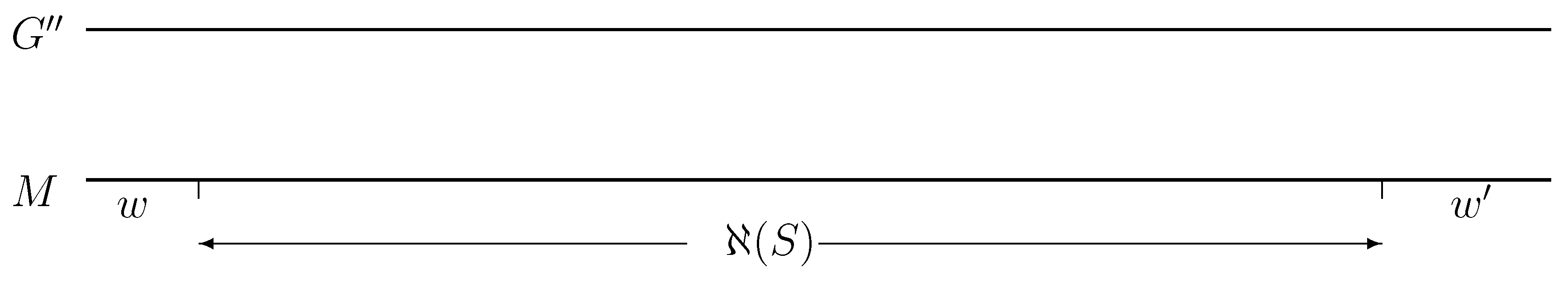
• Define $G_L=\aleph (S_{2i-1}^{\prime })[1,d_{0}logn-1]$ to be the left part of the motif region, $\aleph (S_{2i-1}^{\prime })$.
• Define $G_R=\aleph (S_{2i-1}^{\prime })[|G|-(d_{0}logn)+1,|G|]$ to be the right part of the motif region, $\aleph (S_{2i-1}^{\prime })$.

Lemma 29 shows that with a high probability, Extract-Phase of algorithm Recover-Motif extracts the correct motif regions from the sequences in $Z_1$. It uses $G^{″}$ to match $\aleph (S)$ in another sequences, S. The parameter, R, gives a small probability that the matched region between $G^{″}$ and S is not in $\aleph (S)$.

Lemma 29.

i.

Assume that $G_l$ and $G_r$ are fixed sequences of length $d_{0}logn$. Let S be a $\Theta (n,G,\alpha )$-sequence with $M=\mathrm{Match}(G_l,G_r,S)$, and let $w_0$ be the number of characters of M that are not in the region of $\aleph (S)$. Then, the probability is at most R that $w_0\ge 1$, where R is defined in (xv) of Definition 8.

ii.

The probability is at most $Q_0$ that given a $\Theta (n,G,\alpha )$-sequence S, $\mathrm{Match}(G_L,G_R,S)=\varnothing$.

Proof: 

Assume that $w_0\ge 1$. Let w be the number of characters outside of $\aleph (S)$ on the left of M, and let $w^{\prime }$ be the number of characters outside of $\aleph (S)$ on the right of M. Clearly, $w_0=w+w^{\prime }$. Since $w_0\ge 1$, either $w\ge 1$ or $w^{\prime }\ge 1$. See Figure 1. Without loss of generality, we assume $w\ge 1$.

Figure 1. $G^{″}$ and M.

Statement i: There are two cases.

Case (a): $1\le w<v$. By Lemma 19, the probability for this case is at most $\frac{1}{t}$ for a fixed w. The total probability for this case for $1\le w<v$ is at most ${\sum }_{i=1}^{v-1}\frac{1}{t^i}\le {\sum }_{i=1}^{\infty }\frac{1}{t^i}=\frac{1}{t-1}$.

Case (b): $v\le w$. By Lemma 19, the probability is at most $e^{-\frac{{ϵ}^2}{3}w}$ for a fixed w. The total probability for $v\le w$ is at most ${\sum }_{w=v}^{\infty }{e}^{-\frac{{ϵ}^2}{3}w}=\frac{c^v}{1-c}$.

The probability analysis is similar when $w^{\prime }\ge 1$. Therefore, the probability for this case is at most $R=(\frac{1}{t-1}+\frac{c^v}{1-c})$ for $w_0\ge 1$.

Statement ii: By Lemma 27, with a probability of at most $Q_0$, S does not contain a stable motif region. Therefore, we have a probability of at most $Q_0$ that given a random $\Theta (n,G,\alpha )$-sequence, S, $\mathrm{Match}(G_L,G_R,S)=\varnothing$.   ▮

Lemma 30 shows that we can use $G_l$ and $G_r$ to extract most of the motif regions for the sequences in $Z_2$ if $G^{\prime }=G_L$ (recall that $G_L$ is defined right after Lemma 27).

Lemma 30.

Assume that $G_l$ and $G_r$ are two sequences of a length of $d_{0}logn$, and $G_i=\mathrm{Match}(G_l,G_r,S_i^{″})$ for $S_i^{″}\in Z_2=\{S_1^{″},\cdots ,S_{k_2}^{″}\}$ and $i=1,\cdots ,k_2$ (recall that each sequence, $G_i$, is either an empty sequence or a sequence of the length of $|G_l|$).

i.

If $G_l=G_L$, $G_r=G_R$ and there are no more than $y{k}_2$ ($y\in [0,1]$) sequences, $S_i^{″}$, with ${\mathrm{roughLeft}}_{S_i^{″}}\notin [\mathrm{LB}(S_i^{″})-(v+u_2),\mathrm{LB}(S_i^{″})]$ or ${\mathrm{roughRight}}_{S_i^{″}}\notin [\mathrm{RB}(S_i^{″}),\mathrm{RB}(S_i^{″})+(v+u_2)]$, then the probability is at most $e^{-\frac{{ϵ}^2{k}_2}{3}}$ that there are more than $(Q_0+y+ϵ)k_2$ sequences, $G_i$, with $G_i=\varnothing$.

ii.

For arbitrary $G_l$ and $G_r$, with a probability of at most $e^{-\frac{{ϵ}^2{k}_2}{3}}$, $|\{i|G_i\ne \varnothing \mathrm{and}{G}_i\ne \aleph (S_i^{″}),i=1,\cdots ,k_2\}|>(R+ϵ)k_2$, where R is defined in Definition 8.

Proof: 

Recall that sequence $G_{1L}$ is selected right after Lemma 27.

Statement i: By Lemma 29, for every $S_i^{″}\in Z_2$, the probability is at most $Q_0$ that $S_i^{″}$ does not contain a stable motif region, $\aleph (S_i^{″})$. By Corollary 18, we have a probability of at most $e^{-\frac{{ϵ}^2{k}_2}{3}}$ that there are more than $(Q_0+y+ϵ)k_2$ sequences, $G_i$, with $G_i=\varnothing$.

Statement ii: By Lemma 29, the probability is at most R that $G_i\ne \aleph (S_i^{″})$. By Corollary 18, with a probability of at most $e^{-\frac{{ϵ}^2{k}_2}{3}}$, $|\{i|G_i\ne \aleph (S_i^{″}),i=1,\cdots ,k_2\}|>(R+ϵ)k_2$.   ▮

Definition 31.

• Given two sequences, $G_r$ and $G_r$, define:
  $M(G_r,G_r)=\{G_i^{″}:G_i^{″}=$Match$(G_l,G_r,{\mathrm{roughLeft}}_{S_i^{″}},{\mathrm{roughRight}}_{S_i^{″}},S_i^{″})$$i=1,\cdots ,k_2\}$.
• For a $\Theta (n,G,\alpha )$ sequence, S, define $G_{S,L}$ to be the $\aleph (S)[1,d_{0}logn]$, which is the leftmost subsequence of a length of $d_{0}logn$ in the motif region of S.
• For a $\Theta (n,G,\alpha )$ sequence, S, define $G_{S,R}$ to be the $\aleph (S)[m-d_{0}logn+1,m]$, which is the rightmost subsequence of a length of $d_{0}logn$ in the motif region of S, where $m=|G|=|\aleph (S)|$;

the condition iv of Lemma 32.

Lemma 32.

Assume that we have the following conditions:

i.

For each L with $0<L\le \frac{|G|}{2}$, with a probability of at most ${\varsigma }_1(n)$, $L_{S_i}\notin [{\mathrm{LB}}_{S_i}-2L,{\mathrm{LB}}_{S_i}+2L]$ or $R_{S_i}\notin [{\mathrm{RB}}_{S_i}-2L,{\mathrm{RB}}_{S_i}+2L]$ for $i=1,2$, where $(L_{S_1},R_{S_1},L_{S_2},R_{S_2})=$Collision-Detection($S_1,U_1,S_2,U_2)$, $U_1=$Point-Selection$(S_1,L,[1,|S_1|])$ and $U_2=$Point-Selection$(S_2,L,[1,|S_2|])$.

ii.

For each L with $0<L\le \frac{|G|}{2}$, if $S_1$ has ${\mathrm{roughLeft}}_{S_1}\in [{\mathrm{LB}}_{S_1}-L,{\mathrm{LB}}_{S_1}+L]$ and ${\mathrm{roughRight}}_{S_1}\in [{\mathrm{RB}}_{S_1}-L,{\mathrm{RB}}_{S_1}+L]$, then with a probability of at most ${\varsigma }_2(n)$, $L_{S_i^{″}}\notin [{\mathrm{LB}}_{S_i^{″}}-2L,{\mathrm{LB}}_{S_i^{″}}+2L]$ for $i=1$ or $i=2$, where $(L_{S_1},R_{S_1},L_{S_i^{″}},R_{S_i^{″}})=$ Collision-Detection($S_1,U_1,S_i^{″},U_2)$, $U_1=$ Point-Selection$(S_1,L,[{\mathrm{roughLeft}}_{S_1}-2L,{\mathrm{roughLeft}}_{S_1}+2L])\cup$ Point-Selection$(S_1,L,[{\mathrm{roughRight}}_{S_1}-2L,{\mathrm{roughRight}}_{S_1}+2L])$ and $U_2=$ Point-Selection $(S_i^{″},L,[1,|S_i^{″}|])$.

iii.

The inequality $(P_0+Q_0)<c_0$ holds for some constant $c_0<1$, where $Q_0$ is defined in Equation (13) and $P_0={\varsigma }_1(n)+\frac{2(v+u_1)c^{v+u_1}}{{(1-c)}^2}+\frac{c^v}{1-c}+\frac{1}{5·2^{x}n}$.

iv.

The inequality $1-2(Q_0+V_0+(R+2ϵ))-(\alpha +ϵ)>0$ holds, where $V_0=(2({\varsigma }_2(n)+(v+u_1)\frac{c^{v+u_2}}{1-c}+\frac{c^v}{1-c})+ϵ)$.

Then, the algorithm generates a set of at most $k_2$ subsequences for voting and votes for a sequence, $G^{\prime }$, such that:

(1) with a probability of at most $e^{-\Omega (k_1)}+e^{-\Omega (k_2)}$, $|G^{\prime }|\ne |G|$; and

(2) for each $1\le i\le |G|$, with a probability of at most $e^{-\Omega (k_1)}+e^{-\Omega (k_2)}$, $G^{\prime }[i]\ne G[i]$.

Before proving Lemma 32, we note that both ${\varsigma }_1(n)$ and ${\varsigma }_2(n)$ are at most $\frac{1}{2^x{n}^3}$ for all of the three algorithms. They will be proven by Lemma 47 and Lemma 46 for the case algorithm-type=RANDOMIZED-SUBLINEAR, Lemma 41 and Lemma 40 for the case algorithm-type=RANDOMIZED-SUBQUADRATIC, and Lemma 35 for the case algorithm-type=DETERMINISTIC-SUPERQUADRATIC.

Proof: 

 

By Lemmas 22, with a probability of at most $P_0={\varsigma }_1(n)+\frac{2(v+u_1)c^{v+u_1}}{{(1-c)}^2}+\frac{c^v}{1-c}+\frac{1}{5·2^{x}n}$, ${\mathrm{roughLeft}}_{S_{2i-1}^{\prime }}\notin [\mathrm{LB}(S_{2i-1}^{\prime })-(v+u_1),\mathrm{LB}(S_{2i-1}^{\prime })]$ or ${\mathrm{roughRight}}_{S_{2i-1}^{\prime }}\notin [\mathrm{RB}(S_{2i-1}^{\prime }),\mathrm{RB}(S_{2i-1}^{\prime })+(v+u_1)]$.

By Lemma 23, with a probability of at most $P_a=e^{-{(0.5-P_0-ϵ)}^2{k}_1/3}=e^{-\Omega (k_1)}$, the approximate motif length, $l_{motif}$, is not in the range $[|G|-2(v+u_1),|G|+2(v+u_1)]$. Assume $l_{motif}\in [|G|-2(v+u_1),|G|+2(v+u_1)]$ in the rest of the proof of this lemma.

By Lemma 27, with a probability of at most $Q_0$, a $\Theta (n,G,\alpha )$ sequence does not contain a stable motif region. Therefore, with a probability of at most $P_1={(P_0+Q_0)}^{k_1}$, the following statement is false:

(i) One of $S_{2i-1}^{\prime }$ for $i=1,\cdots ,k_1$ has ${\mathrm{roughLeft}}_{S_{2i-1}^{\prime }}\in [\mathrm{LB}(S_{2i-1}^{\prime })-(v+u_1),\mathrm{LB}(S_{2i-1}^{\prime })]$, ${\mathrm{roughRight}}_{S_{2i-1}^{\prime }}\in [\mathrm{RB}(S_{2i-1}^{\prime }),\mathrm{RB}(S_{2i-1}^{\prime })+(v+u_1)]$ and has a stable motif region.

By Lemma 26, with a probability of at most $P_2=e^{-\frac{{ϵ}^2{k}_2}{3}}$, there are more than $(2({\varsigma }_2(n)+(v+u_1)\frac{c^{v+u_2}}{1-c}+\frac{c^v}{1-c})+ϵ)k_2$ sequences $S_i^{″}$ with ${\mathrm{roughLeft}}_{S_i^{″}}\notin [\mathrm{LB}(S_i^{″})-(v+u_2),\mathrm{LB}(S_i^{″})]$ or ${\mathrm{roughRight}}_{S_i^{″}}\notin [\mathrm{RB}(S_i^{″}),\mathrm{LB}(S_i^{″})+(v+u_2)]$. In other words, with a probability of at most $P_2$, the following statement is false:

(ii) There are no more than $V_0{k}_2$ sequences $S_i^{″}$ with ${\mathrm{roughLeft}}_{S_i^{″}}\notin [\mathrm{LB}(S_i^{″})-(v+u_2),\mathrm{LB}(S_i^{″})]$ or ${\mathrm{roughRight}}_{S_i^{″}}\notin [\mathrm{RB}(S_i^{″}),\mathrm{RB}(S_i^{″})+(v+u_2)]$, where $V_0=(2({\varsigma }_2(n)+(v+u_1)\frac{c^{v+u_2}}{1-c}+\frac{c^v}{1-c})+ϵ)$.

Assume that Statement (ii) is true. By Lemma 30, with a probability of at most $P_3=c^{k_2}$, the following statement is false:

(iii) $M(G_L,G_R)$ contains at most $(Q_0+V_0+ϵ)k_2$ empty sequences.

We start from the rough left boundary, ${\mathrm{roughLeft}}_1$, of $S_1$ to match the other left boundaries of $S_i^{″}$ for $i=1,\cdots ,k_2$. There are in total at most $2(v+u_1)$ candidates to consider.

By Lemma 30, if $M(G_l,G_r)$, which consists of $k_2$ matched regions, has at most $(Q_0+V_0+ϵ)k_2$ empty sequences, then it has more than $(R+ϵ)k_2$ from non-motif regions with a probability of at most$P_4=2(v+u_1)e^{-\frac{{ϵ}^2{k}_2}{3}}$. After the pattern is fixed, those events in the matching are considered to be independent of each other. This is why we can apply the Chernoff bound to deal with them. Therefore, the probability is at most $P_4$; the following statement is false:

(iv) If $M(G_l,G_r)$ contains at most $(Q_0+V_0+ϵ)k_2$ empty sequences, then $M(G_l,G_r)$ contains at most $(Q_0+V_0+ϵ+(R+ϵ))k_2=(Q_0+V_0+(R+2ϵ))k_2$ elements not from motif regions $\{\aleph (S_i^{″}):1\le i\le k_2\}$.

Therefore, with a probability of at most $P_a+P_1+P_2+P_3+P_4=e^{-\Omega (k_1)}+e^{-\Omega (k_2)}$, the sequences are not ready for voting in the next phase, which means the following two conditions are satisfied:

(a) There exists $G_l$ and $G_r$ generated by the algorithm, such that $M(G_l,G_r)$ contains at most $(Q_0+V_0+(R+2ϵ))k_2$ elements not from motif regions $\{\aleph (S_i^{″}):1\le i\le k_2\}$.

(b) For every $G_l$ and $G_r$ that $M(G_l,G_r)$ contains at most $(Q_0+V_0+ϵ)k_2$ empty sequences generated by the algorithm, $M(G_l,G_r)$ contains at most $(Q_0+V_0+ϵ+(R+ϵ))k_2=(Q_0+V_0+(R+2ϵ))k_2$ elements not from motif regions $\{\aleph (S_i^{″}):1\le i\le k_2\}$.

Statement (1): For a $M(G_l,G_r)$ with at most $(Q_0+V_0+(R+2ϵ))k_2$ elements not from motif regions $\{\aleph (S_i^{″}):1\le i\le k_2\}$, we still have $k_2-(Q_0+V_0+(R+2ϵ))k_2$ elements in $M(G_l,G_r)$ from motif regions $\{\aleph (S_i^{″}):1\le i\le k_2\}$. By the condition (iv) in this lemma, we have $k_2-(Q_0+V_0+(R+2ϵ))k_2>(Q_0+V_0+(R+2ϵ))k_2$. Therefore, $|G^{\prime }|$ is selected to be the length of G in the Voting-Phase().

Statement (2): For a $M(G_l,G_r)=\{G_1^{″},\cdots ,G_{k_2}^{″}\}$ with at most $(Q_0+V_0+(R+2ϵ))k_2$ elements not from motif regions $\{\aleph (S_i^{″}):1\le i\le k_2\}$, we still have $k_2-(Q_0+V_0+(R+2ϵ))k_2$ elements in $M(G_l,G_r)$ from motif regions $\{\aleph (S_i^{″}):1\le i\le k_2\}$. By Corollary 18, with a probability of at most $e^{-\frac{{ϵ}^2{k}_2}{3}}$, there are more than $(\alpha +ϵ)k_2$ characters that are mutated in the same position among all $k_2$ motif regions for the sequences in $Z_2$. We have that $k_2-(Q_0+V_0+(R+2ϵ))k_2-(\alpha +ϵ)k_2>(Q_0+V_0+(R+2ϵ))k_2$ by the condition (iv) in this lemma. We let $G^{\prime }[j]$ be the most frequent character among $G_1^{″}[j],\cdots ,G_{k_2}^{″}[j]$ in Voting-Phase. Therefore, with a probability of at most $e^{-\Omega (k_1)}+e^{-\Omega (k_2)}$, $G^{\prime }[j]\ne G[j]$.   ▮

We will use multiple variable functions to characterize the computational time for three algorithms. In order to unify the complexity analysis of three algorithms, we introduce the following notation.

Definition 33.

A function, $T(x,y):N\times N\to N$, is nondecreasing if it is nondecreasing on both variables. If for arbitrary positive constants, $c_1$ and $c_2$, $T(c_{1}x,c_{2}y)\le cT(x,y)$ for some positive constant, c, then $T(x,y)$ is slow.

Lemma 34.

Assume that $t(x,y)$, $s(n,L)$ and $g(n,l)$ are non-decreasing slow functions.Assume that Collision-Detection($S_1,U_1,S_2,U_2$) returns the result in $t(n,||U_1||+||U_2||)$ time and the Point-Selection($S_1,S_2,L)$) selects $s(n,L)$ positions in $g(n,L)$ time. Assume that with a probability of at most $\phi (n)$, the function Initial-Boundaries() does not stop when $L\le |G|/4$, and $||U_{S_{2i-1}^{\prime }}||+||U_{S_j^{″}}||$ in the algorithm Recover-Motif is no more than $f(n,|G|)$.

Then, with a probability of at most $k_1\phi (n)$, the entire algorithm Recover-Motif does not stop in the time complexity $(O(k_1({\sum }_{i=1}^{i_0}(t(n,s(n,\frac{n}{2^i{n}^{2/5}}))+g(n,\frac{n}{2^{i_0}{n}^{2/5}})))+k_1{h}^{2}logn+k_1{k}_{2}t(n,f(n,|G|))+h^{2}logn)+k_1{k}_2(logn)(loglogn)),O(k_2))$, where $i_0$ is the largest j, such that $\frac{n}{2^j{n}^{2/5}}\le min(n^{2/5},|G|)$ and $h=min(n^{2/5},|G|)$.

Proof: 

The function Initial-Boundaries()is executed $k_1$ times. According to the condition that with a probability of at most $\phi (n)$, the function Initial-Boundaries(.) does not stop when $L\le |G|/4$, we have the fact that with a probability of at most $k_1\phi (n)$, one of those executions of Initial-Boundaries(.) does not stop when $L\le |G|/4$.

In the rest of the proof, we assume that all executions of Initial-Boundaries(.) stops when $L\le |G|/4$.

When $L=O(h)$, we detect rough left and right motif boundaries and run Improve-Boundaries(), which takes $O(h^{2}logn)$ time by Lemma 21. It takes $O({\sum }_{i=1}^{i_0}(t(n,s(n,\frac{n}{2^i{n}^{2/5}}))+g(n,\frac{n}{2^i{n}^{2/5}})+h^{2}logn)$ time to run Initial-Boundaries($S_{2i-1}^{\prime },S_{2i}^{\prime }$) one time for one pair ($S_{2i-1}^{\prime },S_{2i}^{\prime }$) in $Z_1$. It takes $O(k_1({\sum }_{i=1}^{i_0}(t(n,s(n,\frac{n}{2^i{n}^{2/5}}))+g(n,\frac{n}{2^i{n}^{2/5}})+k_1{h}^{2}logn)$ time to run Initial-Boundaries($S_{2i-1}^{\prime },S_{2i}^{\prime }$) one time for all pairs ($S_{2i-1}^{\prime },S_{2i}^{\prime }$) in $Z_1$.

It takes $k_2(t(n,f(n,|G|))+h^{2}logn)$ time to find the rough boundaries for all sequences in $Z_2$ with a fixed sequence, S, from $Z_1$ by executing for the loop “For each $S_j^{″}\in Z_2$” in the algorithm Recover-Motif. It takes $k_1{k}_2(t(n,f(n,|G|))+h^{2}logn)$ time to find the rough boundaries for all sequences in $Z_2$ via all sequences, $S_{2i-1}^{\prime }$, from $Z_1$ through the loop “For each $S_j^{″}\in Z_2$” in the algorithm Recover-Motif.

Recall that parameters v and $u_1$ are constants, and $u_2$ is $O(loglogn)$. Calling Match($G_l,G_r,S_i^{″}$) takes $O((v+u_2)logn)$ time for each $S_i^{″}\in Z_2$. The total times for calling Match($G_l,G_r,S_i^{″}$) is $O(k_1{k}_2(v+u_1)(v+u_2)logn)=O(k_1{k}_2(logn)(loglogn))$.

The voting part takes $O(k_2)$ time for executing voting for recovering one character in the motif.   ▮

6.4. Deterministic Algorithm for an $\Omega (1)$ Mutation Rate

In this section, we give a deterministic algorithm for the case with an $\Omega (1)$ mutation rate. The performance of the algorithm is stated in Theorem 6.

Lemma 35.

Let algorithm-type=DETERMINISTIC-SUPERQUADRATIC. Assume that $d_{0}logn\le L\le |G|/2$ and $c_{0}logn\le |G|$. Let $I_1$ be a set of intervals of the positions of $S_1$ that satisfies $[\mathrm{LB}(S_1)-L,\mathrm{LB}(S_1)+L]\cup [\mathrm{RB}(S_1)-L,\mathrm{RB}(S_1)+L]\subseteq {\cup }_{I^{\prime }\in I_1}{I}^{\prime }$. Let $I_2$ be a set of intervals of the positions of $S_2$ that satisfies $[\mathrm{LB}(S_2)-L,\mathrm{LB}(S_2)+L]\cup [\mathrm{RB}(S_2)-L,\mathrm{RB}(S_2)+L]\subseteq {\cup }_{I^{\prime }\in I_2}{I}^{\prime }$. Let $U_1=$ Point-Selection$(S_1,L,I_1)$, $U_2=$ Point-Selection$(S_2,L,I_2)$ and $(L_{S_1},R_{S_1},L_{S_2},R_{S_2})=$ Collision-Detection$(S_1,U_1,S_2,,U_2)$. Then:

i.

with a probability of at most $\frac{1}{2^x{n}^3}$, the left rough boundary, $L_{S_1}$, has at most $d_{0}logn$ distance from $\mathrm{LB}(S_1)$ and the left rough boundary $L_{S_2}$ has at most $d_{0}logn$ distance from $\mathrm{LB}(S_2)$.

ii.

with a probability of at most $\frac{1}{2^x{n}^3}$, the right rough boundary, $R_{S_1}$, has at most $d_{0}logn$ distance from $\mathrm{RB}(S_1)$ and the right boundary of $R_{S_2}$ has at most $d_{0}logn$ distance from $\mathrm{RB}(S_2)$.

Proof: 

For two sequences, $S_1$ and $S_2$, let $\aleph (S_a)$ be the subsequence, $S_a[i_a,j_a]$, for $a=1,2$. By Corollary 18, with a probability of at most $P_l=2c^{d_{0}logn}\le \frac{2}{5·2^x{n}^3}$ (see inequality (8) in Definition 14), there are more than $(\alpha +ϵ)d_{0}logn$ mutations in $S_a[i_a,i_a+d_{0}logn-1]$ for $a=1,2$.

With a probability of at most $P_l$, the left boundary position is missed during the matching. We have similar $P_r=P_l$ to miss the right boundary.

Assume that $p_1$ and $p_2$ are two positions of $S_1$ and $S_2$, respectively. If one of two positions is outside the motif region and has more than $d_{0}logn$ distance to the motif boundary, with a probability of at most $c^{-d_{0}logn}\le \frac{1}{5·2^x{n}^3}$ (see inequality (8) in Definition 14), for them to match requires $\mathrm{diff}(Y_1,Y_2)\le \beta$ by Lemma 19, where $Y_a$ is a subsequence $S_a[p_a,p_a+d_{0}logn-1]$ for $a=1,2$.   ▮

Lemma 36.

For the case algorithm-type=DETERMINISTIC-SUPERQUADRATIC, we have:

i.

Collision-Detection($S_1,U_1,S_2,U_2$) takes $t(n,||U_1||+||U_2||)=O((||U_1||+||U_2{||)}^{2}logn)$ time.

ii.

Point-Selection($S_1,L,[1,|S_1|]$) selects $s(n,L)=O(n)$ positions in $g(n,L)=O(n)$ time.

iii.

$||U_{S_{2i-1}^{\prime }}||+||U_{S_j^{″}}||$ in the algorithm Recover-Motif is no more than $f(n,|G|)=O(|G|+n)$.

iv.

With a probability of at most $\frac{k}{2^x{n}^3}$, the algorithm Recover-Motif does not run in computational complexity $(O(k(n^2{(logn)}^{O(1)}+h^{2}logn)),O(k))$.

Proof: 

Statement i. The parameter, ${\omega }_{\mathrm{DETERMINISTIC}-\mathrm{SUPERQUADRATIC}}$, is set to be β in Collision-Detection. It follows from the time complexity of the brute force method.

Statement ii. It follows from the implementation of Point-Selection().

Statement iii. It follows from the choice of Point-Selection(.) for the sublinear time algorithm at Recover-Motif(.).

Statement iv. It follows from Lemma 34 and Statements i, ii and iii.   ▮

We give the proof for Theorem 6.

Proof: 

[Theorem 6] The computational time part of this theorem follows from Lemma 36.

By Lemma 35, we let ${\varsigma }_1(n)=\frac{1}{2^x{n}^3}\le {\varsigma }_0$ for the probability bound, ${\varsigma }_1(n)$, in the condition (i) of Lemma 32.

By Lemma 35, we can let ${\varsigma }_2(n)=\frac{1}{2^x{n}^3}\le {\varsigma }_0$ for the probability bound, ${\varsigma }_2(n)$, in the condition (i) of Lemma 32

By inequality (12), the condition (iii) of Lemma 32 is satisfied.

By inequality (11), we know that the condition (iv) of Lemma 32 can be satisfied.

The failure probability part of this theorem follows from Lemma 21 and Lemma 32 by using the fact that $k_1,k_2$ and k are of the same order (see equation (18)).   ▮

6.5. Randomized Algorithms for Motif Detection

In this section, we present two randomized algorithms for motif detection. The first one is a sublinear time algorithm that can handle $\frac{1}{{(logn)}^{2+\mu }}$ mutation, and the second one is a super-linear time algorithm that can handle $\Omega (1)$ mutation. They also share some common functions.

Lemma 37.

Let $c_1$ be a constant in $(0,1)$. Assume m and n are two non-negative integers with $m\le n$. Then, for every integer, $m_1$, with $0\le m_1\le \frac{{\delta }_{c_1}m}{lnn}$, $\left(\genfrac{}{}{0pt}{}{n}{m_1}\right)c_1^m\le e^{(mln{c}_1)/2}$, where constant ${\delta }_{c_1}=\frac{-ln{c}_1}{2}$ as defined in Definition 8.

Proof: 

We have the inequalities:

$$\begin{array}{ccc}\hfill \left(\genfrac{}{}{0pt}{}{n}{m_1}\right)c_1^m& \le & n^{m_1}{c}_1^m\hfill \end{array}$$

(23)

$$\begin{array}{ccc}& =& e^{m_{1}lnn}{c}_1^m\hfill \end{array}$$

(24)

$$\begin{array}{ccc}& \le & e^{\frac{{\delta }_{c_1}m}{lnn}lnn}{c}_1^m\hfill \end{array}$$

(25)

$$\begin{array}{ccc}& =& e^{{\delta }_{c_1}m}{e}^{mln{c}_1}\hfill \end{array}$$

(26)

$$\begin{array}{ccc}& =& e^{(mln{c}_1)/2}\hfill \end{array}$$

(27)

   ▮

Lemma 38.

Let $S=U\cup V$ be a set of n elements with $U\cap V=\varnothing$. Assume that $x_1,\cdots ,x_m$ are m random elements in S. Then, with a probability of at most $\left(\genfrac{}{}{0pt}{}{||U||}{m_1}\right){(\frac{||V||+m_1}{n})}^m$, the list, $x_1,\cdots ,x_m$, contains at most $m_1$ different elements from U (in other words, $||\{x_1,\cdots ,x_m\}\cap U||\le m_1$).

Proof: 

For a subset, $S^{\prime }\subseteq S$, with $||S^{\prime }||=m_0$ for some integer, $m_0\ge 0$, the probability is at most ${(\frac{m_0}{n})}^m$ that all elements, $x_1,\cdots ,x_m$, are in $S^{\prime }$. For every subset, $X\subseteq S$, with $||X||\le m_1$, there exists another subset, $S^{\prime }\subseteq S$, such that $||S^{\prime }||=m_1$ and $X\subseteq S^{\prime }$. We have that $\mathrm{Pr}[||\{x_1,\cdots ,x_m\}\cap U||\le m_1]\le \mathrm{Pr}[\{x_1,\cdots ,x_m\}\cap U\subseteq U^{\prime }\mathrm{for}\mathrm{some}{U}^{\prime }\subseteq U\mathrm{with}||U^{\prime }||=m_1]$. There are $\left(\genfrac{}{}{0pt}{}{||U||}{m_1}\right)$ subsets of U with a size of $m_1$. We have the probability of at most $\left(\genfrac{}{}{0pt}{}{||U||}{m_1}\right){(\frac{||V||+m_1}{n})}^m$ that $x_1,\cdots ,x_m$ contains at most $m_1$ different elements in U.   ▮

Lemma 39.

Let β be a constant in $(0,1)$ and $c_1=1-\frac{\beta }{2}$. Let $m_1\le \frac{{\delta }_{c_1}m}{ln\beta n}$ and $m\le n^{1-ϵ}$ for some fixed $ϵ>0$. Let $S_1$ and $S_2$ be two sets of n elements with $||S_1\cap S_2||\ge \beta n$ and C be a set of the size $||C||\le \gamma m_1$ for some constant $\gamma \in (0,1)$. Then, for all large n, with a probability of at most $2e^{-\frac{(1-\gamma )m_{1}m}{n}}$, we have $(A-C)\cap (B-C)=\varnothing$, where $A=\{x_1,\cdots ,x_m\}$ and $B=\{y_1,\cdots ,y_m\}$ are two sets, which may have multiplicities, of m random elements from $S_1$ and $S_2$, respectively.

Proof: 

In the entire proof of this lemma, we always assume that n is sufficiently large. We are going to give an upper bound about the probability that B does not contain any element in $A--C$. For each element, $y_i\in B$, with a probability of at most $1-\frac{||A||-||C||}{n}$, $y_i$ is not in $A--C$. Therefore, the probability is at most ${(1-\frac{||A||-||C||}{n})}^m$ that B does not contain any element in $A--C$.

By Lemma 38, the probability is at most $\left(\genfrac{}{}{0pt}{}{\beta n}{m_1}\right){(\frac{(1-\beta )n+m_1}{n})}^m$ that $||A\cap (S_1\cap S_2)||\le m_1$. We have the inequalities:

$$\begin{array}{ccc}& & \mathrm{Pr}[(A-C)\cap (B-C)=\varnothing ]\hfill \end{array}$$

(28)

$$\begin{array}{ccc}& =& \mathrm{Pr}[(A-C)\cap (B-C)=\varnothing |||A\cap (S_1\cap S_2)||\ge m_1]·\mathrm{Pr}[||A\cap (S_1\cap S_2)||\ge m_1]+\hfill \end{array}$$

(29)

$$\begin{array}{ccc}& & \mathrm{Pr}[(A-C)\cap (B-C)=\varnothing |||A\cap (S_1\cap S_2)||<m_1]·\mathrm{Pr}[|A\cap (S_1\cap S_2)|<m_1]\hfill \end{array}$$

(30)

$$\begin{array}{ccc}& \le & \mathrm{Pr}[(A-C)\cap (B-C)=\varnothing |||A\cap (S_1\cap S_2)||\ge m_1]+\mathrm{Pr}[||A\cap (S_1\cap S_2)||<m_1]\hfill \end{array}$$

(31)

$$\begin{array}{ccc}& \le & {(1-\frac{||A||-||C||}{n})}^m+\left(\genfrac{}{}{0pt}{}{\beta n}{m_1}\right){(\frac{(1-\beta )n+m_1}{n})}^m\hfill \end{array}$$

(32)

$$\begin{array}{ccc}& \le & {(1-\frac{||(A\cap S_1\cap S_2)||-||C||}{n})}^m+\left(\genfrac{}{}{0pt}{}{\beta n}{m_1}\right){(\frac{(1-\beta )n+m_1}{n})}^m\hfill \end{array}$$

(33)

$$\begin{array}{ccc}& \le & {(1-\frac{(1-\gamma )m_1}{n})}^m+\left(\genfrac{}{}{0pt}{}{\beta n}{m_1}\right){(\frac{(1-\beta )n+m_1}{n})}^m\hfill \end{array}$$

(34)

$$\begin{array}{ccc}& \le & e^{-\frac{(1-\gamma )m_{1}m}{n}}+\left(\genfrac{}{}{0pt}{}{\beta n}{m_1}\right){(\frac{(1-\beta )n+m_1}{n})}^m\hfill \end{array}$$

(35)

$$\begin{array}{ccc}& \le & e^{-\frac{(1-\gamma )m_{1}m}{n}}+\left(\genfrac{}{}{0pt}{}{\beta n}{m_1}\right){(1-\frac{\beta }{2})}^m\hfill \end{array}$$

(36)

$$\begin{array}{ccc}& \le & e^{-\frac{(1-\gamma )m_{1}m}{n}}+e^{(mln{c}_1)/2}\hfill \end{array}$$

(37)

$$\begin{array}{ccc}& \le & 2e^{-\frac{(1-\gamma )m_{1}m}{n}}\hfill \end{array}$$

(38)

The inequality, ${(1-\frac{(1-\gamma )m_1}{n})}^m\le e^{-\frac{(1-\gamma )m_{1}m}{n}}$, which is used from Equation (34) to Equation (35), follows from the fact that $1-x\le e^{-x}$. The transition from (35) to (36) follows from the fact that $\frac{m_1}{n}\le \frac{\beta }{2}$, since $m_1=o(n)$, according to the conditions of the lemma.

It is easy to see that $\frac{2(1-\gamma )m_{1}m}{-mln{c}_1}=\frac{2(1-\gamma )m_1}{-ln{c}_1}\le n$ for all large n. Thus, $\frac{(1-\gamma )m_{1}m}{n}\ge (mln{c}_1)/2$ (note that $ln{c}_1<0$ as $c_1\in (0,1)$). Thus, by Lemma 37, $\left(\genfrac{}{}{0pt}{}{\beta n}{m_1}\right){(1-\frac{\beta }{2})}^m\le e^{mln{c}_1/2}\le e^{-\frac{(1-\gamma )m_{1}m}{n}}$. This is why we have the transition from Equation (37) to Equation (38). Therefore, $\mathrm{Pr}[(A-C)\cap (B-C)=\varnothing ]\le 2e^{-\frac{(1-\gamma )m_{1}m}{n}}$.   ▮

6.5.1.. Randomized Algorithm for an $\Omega (1)$ Mutation Rate

In this section, we give an algorithm for the case with an $\Omega (1)$ mutation rate. The performance of the algorithm is stated in Theorem 4.

Lemma 40.

Let algorithm-type=RANDOMIZED-SUBQUADRATIC. Assume that $d_{0}logn\le L\le |G|/2$ and $c_{0}logn\le |G|<\frac{{(logn)}^{3+\tau }}{100}$. Let $I_1$ be a set of intervals of the positions of $S_1$ that satisfy $[\mathrm{LB}(S_1)-L,\mathrm{LB}(S_1)+L]\cup [\mathrm{RB}(S_1)-L,\mathrm{RB}(S_1)+L]\subseteq {\cup }_{I^{\prime }\in I_1}{I}^{\prime }$. Let $I_2$ be a set of intervals of the positions of $S_2$ that satisfy $[\mathrm{LB}(S_2)-L,\mathrm{LB}(S_2)+L]\cup [\mathrm{RB}(S_2)-L,\mathrm{RB}(S_2)+L]\subseteq {\cup }_{I^{\prime }\in I_2}{I}^{\prime }$. Let $U_1=$ Point-Selection$(S_1,L,I_1)$, $U_2=$ Point-Selection$(S_2,L,I_2)$ and $(L_{S_1},R_{S_1},L_{S_2},R_{S_2})=$ Collision-Detection$(S_1,U_1,S_2,,U_2)$. Then:

i.

with a probability of at most $\frac{1}{2^x{n}^3}$, the left rough boundary, $L_{S_1}$, has at most $d_{0}logn$ distance from $\mathrm{LB}(S_1)$ and the left rough boundary, $L_{S_2}$, has at most $d_{0}logn$ distance from $\mathrm{LB}(S_2)$;

ii.

with a probability of at most $\frac{1}{2^x{n}^3}$, the right rough boundary, $R_{S_1}$, has at most $d_{0}logn$ distance from $\mathrm{RB}(S_1)$ and the right boundary of $R_{S_2}$ has at most $d_{0}logn$ distance from $\mathrm{RB}(S_2)$.

Proof: 

The proof is the same as Lemma 35 for the algorithm with algorithm-type=DETERMINISTIC-SUPERQUADRATIC. For two sequences, $S_1$ and $S_2$, let $\aleph (S_a)$ be the subsequence $S_a[i_a,j_a]$ for $a=1,2$. By Corollary 18, with a probability of at most $P_l=2c^{d_{0}logn}\le \frac{2}{5·2^x{n}^3}$ (see inequality (8) in Definition 14), there are more than $(\alpha +ϵ)d_{0}logn$ mutations in $S_a[i_a,i_a+d_{0}logn-1]$ for $a=1,2$.

With a probability of at most $P_l$, the left boundary position is missed during the matching. We have similar $P_r=P_l$ to miss the right boundary.

Assume that $p_1$ and $p_2$ are two positions of $S_1$ and $S_2$, respectively. If one of the two positions is outside the motif region and has more than $d_{0}logn$ distance to the motif boundary, with a probability of at most $c^{-d_{0}logn}\le \frac{1}{5·2^x{n}^3}$ (see inequality (8) in Definition 14), for them to match requires $\mathrm{diff}(Y_1,Y_2)\le \beta$ by Lemma 19, where $Y_a$ is a subsequence $S_a[p_a,p_a+d_{0}logn-1]$ for $a=1,2$.   ▮

Lemma 41.

Let algorithm-type=RANDOMIZED-SUBQUADRATIC. Assume that $d_{0}logn\le L\le |G|/2$ and $|G|\ge \frac{{(logn)}^{3+\tau }}{100}$. Let $I_1$ be a set of intervals of the positions of $S_1$ that satisfy $[\mathrm{LB}(S_1)-L,\mathrm{LB}(S_1)+L]\cup [\mathrm{RB}(S_1)-L,\mathrm{RB}(S_1)+L]\subseteq {\cup }_{I^{\prime }\in I_1}{I}^{\prime }$. Let $I_2$ be a set of intervals of the positions of $S_2$ that satisfy $[\mathrm{LB}(S_2)-L,\mathrm{LB}(S_2)+L]\cup [\mathrm{RB}(S_2)-L,\mathrm{RB}(S_2)+L]\subseteq {\cup }_{I^{\prime }\in I_2}{I}^{\prime }$. Let $U_1=$ Point-Selection$(S_1,L,I_1)$, $U_2=$ Point-Selection$(S_2,L,I_2])$ and $(L_{S_1},R_{S_1},L_{S_2},R_{S_2})=$ Collision-Detection$(S_1,U_1,S_2,U_2)$. Then:

i.

with a probability of at most $\frac{1}{2^x{n}^3}$, the left rough boundary, $L_{S_1}$, has at most a $2L$ distance from $\mathrm{LB}(S_1)$ and the left rough boundary $L_{S_2}$ has at most a $2L$ distance from $\mathrm{LB}(S_2)$;

ii.

with a probability of at most $\frac{1}{2^x{n}^3}$, the right rough boundary, $R_{S_1}$, has at most a $2L$ distance from $\mathrm{RB}(S_1)$ and the right boundary of $R_{S_2}$ has at most a $2L$ distance from $\mathrm{RB}(S_2)$.

Proof: 

We prove the following two statements which imply the lemma.

i.

With a probability of at most $\frac{1}{2^x{n}^3}$, there are no intervals, $A_i$ from $S_1$ and $B_j$ from $S_2$, such that: (1) $||A_i(S_1,\aleph (S_1))\cap B_j(S_2,\aleph (S_2))||$ is at least $\frac{L}{2}$; (2) the left boundary of $S_1$ has at most a $2L$ distance from $A_i$; (3) the left boundary of $S_2$ has at most a $2L$ distance from $B_j$; and (4) there is a collision between the sampled positions in $A_i$ and $B_j$.

ii.

With a probability pf at most $\frac{1}{2^x{n}^3}$, there are no intervals, $A_i$ from $S_1$ and $B_j$ from $S_2$, such that: (1) $||A_i(S_1,\aleph (S_1))\cap B_j(S_2,\aleph (S_2))||$ is at least $\frac{L}{2}$; (2) the right boundary of $S_1$ has at most a $2L$ distance from $A_i$; (3) the right boundary of $S_2$ has at most a $2L$ distance from $B_j$; and (4) there is a collision between the sampled positions in $A_i$ and $B_j$.

We only prove statement i. The proof for statement ii is similar.

Select $A_i$ from $S_1$ and $B_j$ from $S_2$ to be the first pair of intervals with $||A_i(S_1,\aleph (S_1))\cap B_j(S_2,\aleph (S_2))||\ge \frac{L}{2}$. It is easy to see that such a pair exists, and both have a distance from the left boundary with a distance of at most $2L$. This is because when a leftmost interval of a length pf L is fully inside the motif region of the first sequence, we can always find the second interval from the second sequence with an intersection of a length of at least $\frac{L}{2}$.

Replace m by $M(L)$, $m_1$ by $M_1(L)$ (see Definition 10) and n by L to apply Lemma 39. We do not consider any damaged position in this algorithm; therefore, let C be empty.

With a probability of at most $o(\frac{1}{2^x{n}^3})$, there is a point in $(A_i(S_1,\aleph (S_1))-C)\cap (B_j(S_2,\aleph (S_2))-C)$. The subsequences of a length of $d_{0}logn$ starting at the point from $S_1$ and $S_2$ fail to have the difference bounded by β with a probability of at most $o(\frac{1}{2^x{n}^3})$ by Lemma 20. With a probability of at most $o(\frac{1}{2^x{n}^3})$, we do not have that the rough boundaries are detected with a distance of at most $2L$ to exact motif boundaries.   ▮

Lemma 42.

For the case algorithm-type=RANDOMIZED-SUBQUADRATIC, we have:

i.

Collision-Detection($S_1,U_1,S_2,U_2$) takes $t(n,||U_1||+||U_2||)=O((||U_1||+||U_2{||)}^{2}logn)$ time.

ii.

Point-Selection($S_1,L,[1,|S_1|]$) selects $s(n,L)=O((\frac{n}{L})M(L))$ positions in $g(n,L)=O(s(n,L))$ time if $L\ge \frac{{(logn)}^{3+\tau }}{100}$.

iii.

Point-Selection($S_1,L,[1,|S_1|]$) selects $s(n,L)=O(n)$ positions in $g(n,L)=O(n)$ time if $L<\frac{{(logn)}^{3+\tau }}{100}$.

iv.

$||U_{S_{2i-1}^{\prime }}||+||U_{S_j^{″}}||$ in the algorithm Recover-Motif is no more than $f(n,|G|)=O(M(|G|)+\frac{n}{|G|}M(|G|))$.

v.

With a probability of at most $\frac{k}{2^x{n}^3}$, the algorithm Recover-Motif does not stop in $(O(k(\frac{n^2}{|G|}{(logn)}^{O(1)}+h^{2}logn)),O(k))$ time.

Proof: 

Statement i. The parameter, ${\omega }_{\mathrm{RANDOMIZED}-\mathrm{SUBLINEAR}}$, is set to be β in Collision-Detection. It follows from the time complexity of the brute force method.

Statements ii and iii. They follow from the implementation of Point-Selection().

Statement iv. It follows from the choice of Point-Selection(.) for the sublinear time algorithm at Recover-Motif(.).

Statement iv. It follows from Lemma 40, Lemma 34 and Statements i, ii and iii.   ▮

We give the proof for Theorem 6.

Proof: 

[Theorem 4] The computational time part of this theorem follows from Lemma 42.

By Lemma 40, we can let ${\varsigma }_1(n)=\frac{1}{2^x{n}^3}\le {\varsigma }_0$ for the probability bound, ${\varsigma }_1(n)$, in the condition (i) of Lemma 32.

By Lemma 41, we can let ${\varsigma }_2(n)=\frac{1}{2^x{n}^3}\le {\varsigma }_0$ for the probability bound, ${\varsigma }_2(n)$, in the condition (ii) of Lemma 32.

By inequality (12), the condition (iii) of Lemma 32 is satisfied.

By inequality (11), we know that the condition (iii) of Lemma 32 can be satisfied.

The failure probability part of this theorem follows from Lemma 21 and Lemma 32 by using the fact that $k_1,k_2$ and k are of the same order (see Equation (18)).   ▮

6.5.2.. Sublinear Time Algorithm for a $\frac{1}{{(logn)}^{2+\mu }}$ Mutation Rate

In this section, we give an algorithm for the case with at most $\alpha =\frac{1}{{(logn)}^{2+\mu }}$ mutation rate. The performance of the algorithm is stated in Theorem 2.

Definition 43.

A position, p, in the motif region, $\aleph (S)$, of an input sequence, S, is damaged if there exists at least one mutation in $S[p,p+d_{0}logn-1]$, where $d_0$ is defined in item (xvii) in Definition 8.

Lemma 44.

Assume that $\alpha L={(logn)}^{1+\Omega (1)}$. With a probability of at most $e^{-{(logn)}^{1+\Omega (1)}}$, there are more than $\frac{M_1(L)}{{(logn)}^{\Omega (1)}}$ positions that are from the $M(L)$ (see Definition 10 for $M(.)$ and $M_1(.)$) sampled positions that are damaged in an interval of a length pf L.

Proof: 

By Theorem 16, with a probability of at most $P_1=2^{-\alpha L}$ (let $\delta =2$), there are more than $3\alpha L$ mutations in an interval of a length of L. Therefore, with a probability of at most $2^{-\alpha L}=e^{-{(logn)}^{1+\Omega (1)}}$, there are more than $3\alpha Llogn$ positions that are damaged. Therefore, each random position in an interval of a length of L has at most a probability of $\frac{3\alpha Llogn}{L}=3\alpha logn$ to be damaged.

Since $\alpha =(\frac{1}{{(logn)}^{2+\Omega (1)}})$ and $M(L)$ positions are sampled, by Theorem 16, with a probability of at most $P_2=2^{-(3\alpha logn)M(L)}=e^{-{(logn)}^{1+\Omega (1)}}$ (let $\delta =2$), the number of damaged positions sampled in an interval of a length of L is more than $((1+\delta )3\alpha logn)M=(9\alpha logn)M(L)=\frac{M_1(L)}{{(logn)}^{\Omega (1)}}$. Thus, with a total probability of at most $P_1+P_2=e^{-{(logn)}^{1+\Omega (1)}}$, there are more than $\frac{M_1(L)}{{(logn)}^{\Omega (1)}}$ damaged positions that are from the $M(L)$ sampled positions in an interval of a length of L.   ▮

Definition 45.

Let A be a set of positions in an input sequence, S, with $\aleph (S)=S[i,j]$. Let $A(S,\aleph (S))=\{x-i+1|x\in A\cap [i,j]\}$. In other words, $A(S,\aleph (S))$ contains all the positions of A in $\aleph (S)$.

Lemma 46. Let

Let algorithm-type=RANDOMIZED-SUBLINEAR. Assume that$|G|<\frac{{(logn)}^{3+\tau }}{100}$ and L is an integer with $d_{0}logn\le L\le |G|/2$. Let $I_1$ be a set of intervals of the positions of $S_1$ that satisfy $[\mathrm{LB}(S_1)-L,\mathrm{LB}(S_1)+L]\cup [\mathrm{RB}(S_1)-L,\mathrm{RB}(S_1)+L]\subseteq {\cup }_{I^{\prime }\in I_1}{I}^{\prime }$. Let $I_2$ be a set of intervals of the positions of $S_2$ that satisfy $[\mathrm{LB}(S_2)-L,\mathrm{LB}(S_2)+L]\cup [\mathrm{RB}(S_2)-L,\mathrm{RB}(S_2)+L]\subseteq {\cup }_{I^{\prime }\in I_2}{I}^{\prime }$. Let $U_1=$ Point-Selection$(S_1,L,I_1)$, $U_2=$ Point-Selection$(S_2,L,I_2])$ and $(L_{S_1},R_{S_1},L_{S_2},R_{S_2})=$ Collision-Detection$(S_1,U_1,S_2,U_2)$. Then:

i.

with a probability of at most $\frac{1}{2^x{n}^3}$, the left rough boundary, $L_{S_1}$, has at most a $|G|/4$ distance from $\mathrm{LB}(S_1)$ and the left rough boundary, $L_{S_2}$, has at most a $|G|/4$ distance from $\mathrm{LB}(S_2)$.

ii.

with a probability of at most $\frac{1}{2^x{n}^3}$, the right rough boundary, $R_{S_1}$, has at most a $|G|/4$ distance from $\mathrm{RB}(S_1)$ and the right boundary of $R_{S_2}$ has at most a $|G|/4$ distance from $\mathrm{RB}(S_2)$.

Proof: 

For two sequences, $S_1$ and $S_2$, it is easy to see that there is a common position in both motif regions of the two sequences, such that there is no mutation in the next $d_{0}logn$ characters with a high probability. This is because that mutation probability is small.

By Theorem 16, with a probability of at most $P_l=2^{-\alpha |G|/4}$ (let $\delta =2$), there are more than $3\alpha \frac{|G|}{4}$ mutated characters in the interval $\aleph (S_i)[1,\frac{|G|}{4}]$ for $i=1,2$. Since the mutation probability is $\alpha =(\frac{1}{{(logn)}^{2+\Omega (1)}})$, with a probability of at most $2^{-\alpha |G|/4}=e^{-{(logn)}^{1+\Omega (1)}}$, there are more than $3\alpha ·\frac{|G|}{4}{d}_{0}logn$ positions to be damaged in $\aleph (S_i)[1,\frac{|G|}{4}]$.

Similarly, we have a probability of at most $P_r=e^{-{(logn)}^{1+\Omega (1)}}$ that there are more than $((3\alpha d_{0}logn)·\frac{|G|}{4})=\frac{|G|}{{(logn)}^{\Omega (1)}}$ damaged positions in $\aleph (S_i)[\frac{3|G|}{4}-1,|G|]$.

Now, we assume that left side has more than $((3\alpha d_{0}logn)·\frac{|G|}{4})=\frac{|G|}{{(logn)}^{\Omega (1)}}$ damaged positions and the right side, more than $((3\alpha d_{0}logn)·\frac{|G|}{4})=\frac{|G|}{{(logn)}^{\Omega (1)}}$ damaged positions in $\aleph (S_i)[\frac{3|G|}{4}-1,|G|]$. Since each position in each interval of a length of L is selected in Point-Selection$(S_1,S_2,L)$, it is easy to verify the conclusions of this lemma.   ▮

Lemma 47.

Let algorithm-type=RANDOMIZED-SUBLINEAR. Assume that $|G|\ge \frac{{(logn)}^{3+\tau }}{100}$ and $d_{0}logn\le L\le |G|/2$. Let $I_1$ be a set of intervals of the positions of $S_1$ that satisfy $[\mathrm{LB}(S_1)-L,\mathrm{LB}(S_1)+L]\cup [\mathrm{RB}(S_1)-L,\mathrm{RB}(S_1)+L]\subseteq {\cup }_{I^{\prime }\in I_1}{I}^{\prime }$. Let $I_2$ be a set of intervals of the positions of $S_2$ that satisfy $[\mathrm{LB}(S_2)-L,\mathrm{LB}(S_2)+L]\cup [\mathrm{RB}(S_2)-L,\mathrm{RB}(S_2)+L]\subseteq {\cup }_{I^{\prime }\in I_2}{I}^{\prime }$. Let $U_1=$Point-Selection$(S_1,L,I_1)$, $U_2=$Point-Selection$(S_2,L,I_2])$ and $(L_{S_1},R_{S_1},L_{S_2},R_{S_2})=$Collision-Detection$(S_1,U_1,S_2,U_2)$. Then:

i.

with a probability of at most $\frac{1}{2^x{n}^3}$, the left rough boundary, $L_{S_1}$, has at most a $2L$ distance from $\mathrm{LB}(S_1)$ and the left rough boundary, $L_{S_2}$, has at most a $2L$ distance from $\mathrm{LB}(S_2)$.

ii.

With a probability of at most $\frac{1}{2^x{n}^3}$, the right rough boundary, $R_{S_1}$, has at most a $2L$ distance from $\mathrm{RB}(S_1)$ and the right boundary of $R_{S_2}$ has at most a $2L$ distance from $\mathrm{RB}(S_2)$.

Proof: 

We prove the following two statements, which imply the lemma.

i.

With a probability of at most $\frac{1}{2^x{n}^3}$, there are no intervals, $A_i$ from $S_1$ and $B_j$ from $S_2$, such that: (1) $||A_i(S_1,\aleph (S_1))\cap B_j(S_2,\aleph (S_2))||$ is at least $\frac{L}{2}$; (2) the left boundary of $S_1$ has at most a $2L$ distance from $A_i$; (3) the left boundary of $S_2$ has at most a $2L$ distance from $B_j$; and (4) there is a collision between the sampled positions in $A_i$ and $B_j$.

ii.

with a probability of at most $\frac{1}{2^x{n}^3}$, there are no intervals, $A_i$ from $S_1$ and $B_j$ from $S_2$, such that: (1) $||A_i(S_1,\aleph (S_1))\cap B_j(S_2,\aleph (S_2))||$ is at least $\frac{L}{2}$; (2) the right boundary of $S_1$ has at most a $2L$ distance from $A_i$; (3) the right boundary of $S_2$ has at most a $2L$ distance from $B_j$; and (4) there is a collision between the sampled positions in $A_i$ and $B_j$.

We only prove statement i. The proof for statement ii is similar to that for statement i. Assume that L satisfies the condition of this lemma. Select $A_i$ from $S_1$ and $B_j$ from $S_2$ to be the first pair of intervals of a size of L with $||A_i(S_1,\aleph (S_1))\cap B_j(S_2,\aleph (S_2))||\ge \frac{L}{2}$. This is because when a leftmost interval of a length of L is fully inside the motif region of the first sequence, we can always find the second interval from the second sequence with an intersection of a length of at least $\frac{L}{2}$.

Replace m by $M(L)$, $m_1$ by $M_1(L)$ (see Definition 10) and n by L to apply Lemma 39. We also let C be the set of damaged positions in $\aleph (S_1)$ and $\aleph (S_2)$ caused by the mutated positions. With a probability of at most $o(\frac{1}{2^x{n}^3})$, C has a size of $o(M_1(L))$ by Lemma 44. With a probability of at most $o(\frac{1}{2^x{n}^3})$, there is point in $(A_i(S_1,\aleph (S_1))-C)\cap (B_j(S_2,\aleph (S_2))-C)$. The existence of such a point makes $L_{S_1}$ and $L_{S_2}$ have a distance of at most $2L$ to $\mathrm{LB}(S_1)$ and $\mathrm{LB}(S_2)$, respectively.   ▮

Lemma 48.

For the case algorithm-type=RANDOMIZED-SUBLINEAR, we have:

i.

Collision-Detection($S_1,U_1,S_2,U_2$) takes $t(n,||U_1||+||U_2||)=O((||U_1||+||U_2||)logn)$ time.

ii.

Point-Selection($S_1,L,[1,|S_1|]$) selects $s(n,L)=O((\frac{n}{L})M(L))$ positions in $g(n,L)=O(s(n,L))$ time if $L\ge \frac{{(logn)}^{3+\tau }}{100}$.

iii.

Point-Selection($S_1,L,[1,|S_1|]$) selects $s(n,L)=O(n)$ positions in $g(n,L)=O(n)$ time if $L<\frac{{(logn)}^{3+\tau }}{100}$.

iv.

$||U_{S_{2i-1}^{\prime }}||+||U_{S_j^{″}}||$ in the algorithm Recover-Motif is no more than $f(n,|G|)=O(M(|G|)+\frac{n}{|G|}M(|G|))$.

v.

With a probability of at most $\frac{k}{2^x{n}^3}$, the algorithm Recover-Motif does not stop in $(O(k(\frac{n}{\sqrt{h}}{(logn)}^{\frac{5}{2}}+h^{2}logn)),O(k))$ time.

Proof: 

Statement i. The parameter, ${\omega }_{\mathrm{RANDOMIZED}-\mathrm{SUBLINEAR}}$, is set to be zero in Collision-Detection. It follows from the time complexity of bucket sorting, which is described in standard algorithm textbooks.

Statements ii and iii. They follow from the implementation of Point-Selection().

Statement iv. It follows from the choice of Point-Selection(.) for the sublinear time algorithm at Recover-Motif(.).

Statement v. It follows from Lemma 46, Lemma 47 and Lemma 34 and Statements i, ii iii and iv.   ▮

We give the proof for Theorem 2.

Proof: 

[Theorem 2] The computational time part of this theorem follows from Lemma 48.

By Lemma 46, we can let ${\varsigma }_1(n)=\frac{1}{2^x{n}^3}\le {\varsigma }_0$ for the probability bound, ${\varsigma }_1(n)$, in the condition (i) of Lemma 32.

By Lemma 47, we can let ${\varsigma }_2(n)=\frac{1}{2^x{n}^3}\le {\varsigma }_0$ for the probability bound, ${\varsigma }_1(n)$, in the condition (ii) of Lemma 32.

By inequality (12), the condition (iii) of Lemma 32 is satisfied.

By inequality (11), we know that the condition (iv) of Lemma 32 can be satisfied.

The failure probability part of this theorem follows from Lemma 21 and Lemma 32 by using the fact that $k_1,k_2$ and k are of the same order (see Equation (18)).   ▮

6.6. Experiments on Simulated Datasets

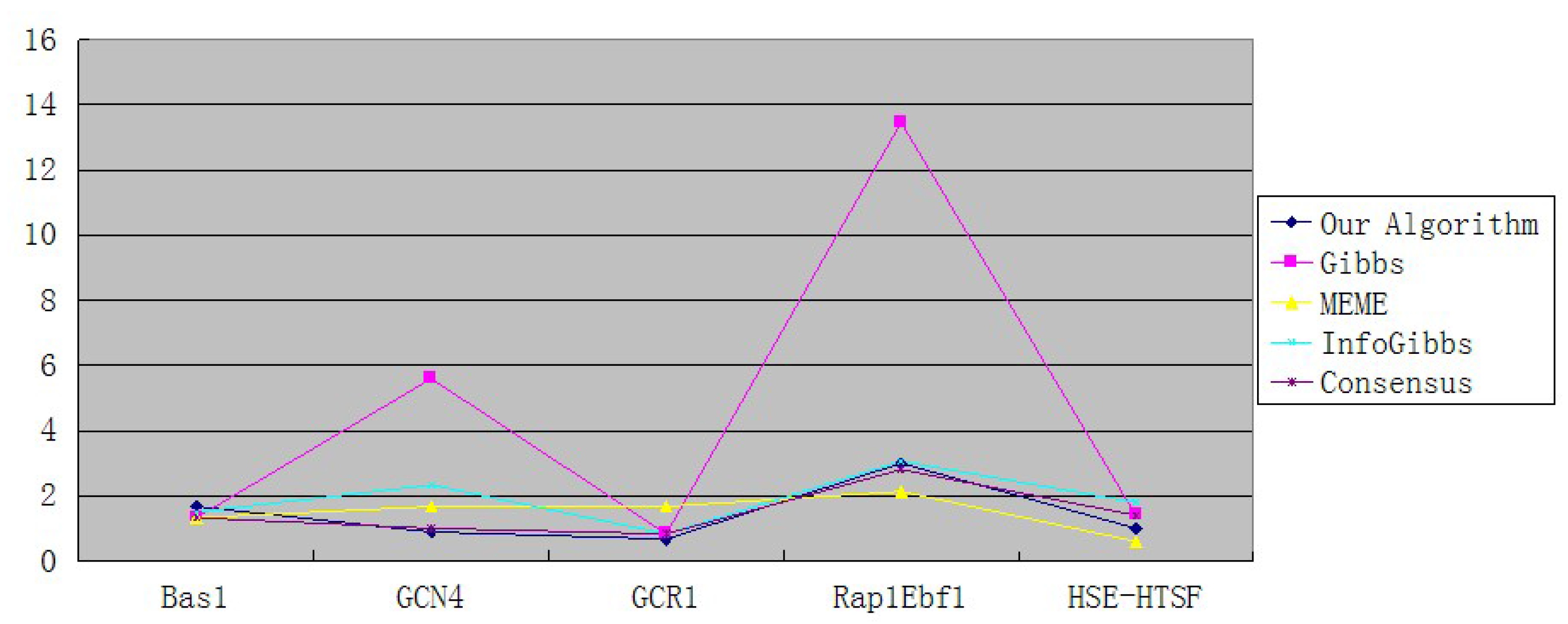
Aiming at solving the motif discovery problem, we implemented our algorithm in Java. Our tests were all done on a laptop with an Intel Dual Core 1.5 G CPU and 3.0 G Memory. In the first experiment, we tested our algorithm on several simulated datasets, which are all generated from our probability model with a small mutation rate. Each input set contains 20 or 15 sequences, which are of a length of 600 or 500 base pairs. Additionally, each bp of all the simulated gene sequences was generated independently with the same occurrence probability. A motif with a fixed length was randomly planted into each input sequence. The minimum Hamming distances between the results and consensus are recorded.

6.7. Experiments

There are many other tools for detecting and analyzing the motifs, like the EMmethod [23], MEME [24], Gibbs [25], Compo [26], MochiView [27], PhyME [28], HeliCis [29] and WebMotif [30], among others. Each of them has their advantages and disadvantages.

Table 1 shows the results on simulated datasets. From the table, we could find that the results of our algorithm for finding the motif on simulated datasets are satisfied. Our algorithm could find all the motifs from each sequence and get the consensus with an accuracy rate of 100%. If the dataset has a high mutation rate, we could increase the number of repetitions, so that the result on the datasets will be more accurate. We also recorded the total time cost for each test, which mainly depends on the number of test repetitions. In the experimental tables, the parameter, N, represents the number of sequences, parameter M represents the length of motifs, parameter M is the maximum length of sequences and R is the number of iterations. GCR1 is a famous DNA binding protein, whose ability to bind DNA is dependent on the CTTCC sequence motif [31]. Several other popular data sets are also used in the experiments of our motif detection and its comparisons to the other methods.

Table 1. Results on simulated data.

	N	M	L	R	Accuracy Rate	Time cost(s)
Set 1	20	600	15	60	100	98
Set 2	15	600	15	10	100	18
Set 3	20	600	12	15	100	22
Set 4	20	500	15	40	100	79

Table 1. Results on simulated data.

	N	M	L	R	Accuracy Rate	Time cost(s)
Set 1	20	600	15	60	100	98
Set 2	15	600	15	10	100	18
Set 3	20	600	12	15	100	22
Set 4	20	500	15	40	100	79

In the second experiment, we tested our algorithm on a real sequence set, which was obtained from SCPD. SCPD contains a large number of gene data and transcription factors of yeast. Sequences in the same set are all regulated by a common motif. We chose 1,000 bp as the length of the input sequences. In order to show the advantages of our algorithm, we also compared the result of our algorithm with the results of several other existing motif finding methods on the same dataset, such as Gibbs, MEME, Info-Gibbs and Consensus. Table 2 shows the details of the data set we used in the experiment.

Table 2. Number of Sequences and Motif Length.

	Bas1	GCN4	GCR1	Rap1Ebf1	HSE-HTSF
N	6	9	6	15	5
L	10	10	10	15	10

Table 2. Number of Sequences and Motif Length.

	Bas1	GCN4	GCR1	Rap1Ebf1	HSE-HTSF
N	6	9	6	15	5
L	10	10	10	15	10

Table 3 shows the results of the five algorithms on biological data sets. Table 4 and Figure 2 give the average mismatch numbers of each algorithm. We choose four well-known motif-detecting softwares to make the comparisons. From Table 3 and Table 4, we see that the average mismatch numbers of our algorithm on data sets GCN4 and GCR1 are significantly lower than other four well-known methods. On the data sets Bas1,Rap1Ebf1 and HSE-HTSF, our algorithms also shows satisfied performance compared to other methods.

In addition, our algorithm also shows its high speed in computations compared to other four motif finding methods. Because the starting pattern of algorithms are represented by a string, so our algorithm can avoid some extra time consuming computations unlike Gibbs sampling and EM methods, such as computations of likelihoods. According to this feature, we use the consensus string of the voting operation obtained from the last iteration as a new starting pattern in program, and continue doing voting operations repeatedly until there is no further improvement. Experimental results show that if we set the number of iterations to be a large integer, the programs could give more accurate results within a reasonable time.

Table 3. Total number of mismatch positions.

	Bas1	GCN4	GCR1	Rap1Ebf1	HSE-HTSF
Our Algorithm	10	8	4	45	5
Gibbs	8	51	5	202	7
MEME	8	15	10	32	3
InfoGibbs	9	21	5	46	9
Consensus	8	9	5	42	7

Table 3. Total number of mismatch positions.

	Bas1	GCN4	GCR1	Rap1Ebf1	HSE-HTSF
Our Algorithm	10	8	4	45	5
Gibbs	8	51	5	202	7
MEME	8	15	10	32	3
InfoGibbs	9	21	5	46	9
Consensus	8	9	5	42	7

Table 4. Average mismatch numbers per sequence.

	Bas1	GCN4	GCR1	Rap1Ebf1	HSE-HTSF
Our Algorithm	1.67	0.89	0.67	3	1
Gibbs	1.33	5.6	0.83	13.46	1.4
MEME	1.33	1.67	1.67	2.13	0.6
InfoGibbs	1.5	2.33	0.83	3.06	1.8
Consensus	1.33	1	0.83	2.8	1.4

Table 4. Average mismatch numbers per sequence.

	Bas1	GCN4	GCR1	Rap1Ebf1	HSE-HTSF
Our Algorithm	1.67	0.89	0.67	3	1
Gibbs	1.33	5.6	0.83	13.46	1.4
MEME	1.33	1.67	1.67	2.13	0.6
InfoGibbs	1.5	2.33	0.83	3.06	1.8
Consensus	1.33	1	0.83	2.8	1.4

Figure 2. Average mismatch numbers per sequence.

6.8. Conclusions

We develop algorithms under the probabilistic model. One of them finds the implanted motif with a high probability if the alphabet size is at least four, the motif length is in $[{(logn)}^{7+\mu },\frac{n}{{(logn)}^{1+\mu }}]$ and each character in the motif region has a probability of at most $\frac{1}{{(logn)}^{2+\mu }}$ of mutation. The motif region can be detected, and each motif character can be recovered in sublinear time. A sub-quadratic randomized algorithm is developed to recover the motif with an $\Omega (1)$ mutation rate. A quadratic deterministic algorithm is developed to recover the motif with an $\Omega (1)$ mutation rate. It is an interesting problem if there is an algorithm to handle the case for an alphabet of a size of three. A more interesting problem is to extend the algorithm to handle larger mutation probability.

6.9. Future Works

Compared with other motif finding methods, our algorithm shows its great advantages. However, there are still some improvements that could be done on this algorithm. For example, though a sequence set has the consensus, the motif in each sequence may have high mutation rates; in addition, the length of each motif could also be different. Therefore, these two factors increase the difficulty for finding motifs, and currently, there is still no effective algorithm that could solve these problems. In the future, we plan to improve the efficiency of our algorithm by combining other motif finding methods, such as MEME; a combination may be made to make our algorithm have better performance in finding motifs from highly mutated sequences.

References

- Frances, M.; Litman, A. On covering problems of codes. Theor. Comput. Sci. 1997, 30, 113–119. [Google Scholar] [CrossRef]
- Ga̧sieniec, L.; Jansson, J.; Lingas, A. Efficient Approximation Algorithms for the Hamming Center Problem. In Proceedings of the 10th Annual ACM-SIAM Symposium on Discrete Algorithms, Baltimore, MD, USA, 17–19 January 1999; pp. S905–S906.
- Stormo, G.; Hartzell, G., III. Identifying protein-binding sites from unaligned DNA fragments. Proc. Natl. Acad. Sci. USA 1991, 88, 5699–5703. [Google Scholar] [CrossRef] [PubMed]
- Lawrence, C.; Reilly, A. An expectation maximization (EM) algorithm for the identification and characterization of common sites in unaligned biopolymer sequences. Proteins 1990, 7, 41–51. [Google Scholar] [CrossRef] [PubMed]
- Hertz, G.; Stormo, G. Identification of Consensus Patterns in Unaligned DNA and Protein Sequences: A Large-Deviation Statistical Basis for Penalizing Gaps. In Proceedings of the 3rd International Conference on Bioinformatics and Genome Research, Tallahassee, USA, 1–4 June 1994; pp. 201–216.
- Stormo, G. Consensus patterns in DNA. In Molecular Evolution: Computer Analysis of Protein and Nucleic Acid Sequences; Doolitle, R.F., Ed.. Methods Enzymol. 1990, 183, 211–221. [Google Scholar]
- Lanctot, J.K.; Li, M.; Ma, B.; Wang, L.; Zhang, L. Distinguishing string selection problems. Inf. Comput. 2003, 185, 41–55. [Google Scholar] [CrossRef]
- Lucas, K.; Busch, M.; Mossinger, S.; Thompson, J. An improved microcomputer program for finding gene- or gene family-specific oligonucleotides suitable as primers for polymerase chain reactions or as probes. Comput. Appl. Biosci. 1991, 7, 525–529. [Google Scholar] [CrossRef] [PubMed]
- Dopazo, J.; Rodríguez, A.; Sáiz, J.C.; Sobrino, F. Design of primers for PCR amplification of highly variable genomes. Comput. Appl. Biosci. 1993, 9, 123–125. [Google Scholar] [PubMed]
- Proutski, V.; Holme, E.C. Primer master: A new program for the design and analysis of PCR primers. Comput. Appl. Biosci. 1996, 12, 253–255. [Google Scholar] [CrossRef] [PubMed]
- Li, M.; Ma, B.; Wang, L. On The Closest String and Substring Problems. J. ACM 2002, 49, 157–171. [Google Scholar] [CrossRef]
- Li, M.; Ma, B.; Wang, L. Finding Similar Regions in Many Strings. In Proceedings of the 31st Annual ACM Symposium on Theory of Computing, Atlanta, GA, USA, 1–4 May 1999; pp. 473–482.
- Pevzner, P.; Sze, S. Combinatorial Approaches to Finding Subtle Signals in DNA Sequences. In Proceedings of the 8th International Conference on Intelligent Systems for Molecular Biology, Toronto, ON, Canada, 19–23 July 2000; pp. 269–278.
- Keich, U.; Pevzner, P. Finding motifs in the twilight zone. Bioinformatics 2002, 18, 1374–1381. [Google Scholar] [CrossRef] [PubMed]
- Keich, U.; Pevzner, P. Subtle motifs: Defining the limits of motif finding algorithms. Bioinformatics 2002, 18, 1382–1390. [Google Scholar] [CrossRef] [PubMed]
- Wang, L.; Dong, L. Randomized algorithms for motif detection. J. Bioinform. Comput. Biol. 2005, 3, 1039–1052. [Google Scholar] [CrossRef] [PubMed]
- Chin, F.; Leung, H. Voting Algorithms for Discovering Long Motifs. In Proceedings of the 3rd Asia-Pacific Bioinformatics Conference, Singapore, 17–21 January 2005; pp. 261–272.
- Gusfield, D. Algorithms on Strings, Trees, and Sequences; Cambridge University Press: Cambridge, UK, 1997. [Google Scholar]
- Fu, B.; Kao, M.Y.; Wang, L. Probabilistic analysis of a motif discovery algorithm for multiple sequences. SIAM J. Discret. Math. 2009, 23, 1715–173. [Google Scholar] [CrossRef]
- Fu, B.; Kao, M.Y.; Wang, L. Discovering almost any hidden motif from multiple sequences. ACM Transactions on Algorithms 2011, 7(2), 26. [Google Scholar] [CrossRef]
- Liu, X.; Ma, B.; Wang, L. Voting Algorithms for the Motif Problem. In Proceedings of Computational Systems Bioinformatics Conference, (CSB’08), Stanford, CA, USA, 26–29 August 2008; pp. 37–47.
- Motwani, R.; Raghavan, P. Randomized Algorithms; Cambridge University Press: Cambridge, UK, 2000. [Google Scholar]
- Dempster, A.P.; Laird, N.M.; Rubin, D.B. Maximum likelihood from complete data vis the EM algorithm. J. R. Stat. Soc. 1977, 39, 1–38. [Google Scholar]
- D’haesler, P. How does DNA sequence motif discovery work? Nat. Biotechnol. 2006, 24, 959–961. [Google Scholar] [CrossRef] [PubMed]
- Lawrence, C.; Altschul, S.; Boguski, M.; Liu, J.; Neuwald, A.; Wootton, J. Detecting subtle sequence signals: A gibbs sampling strategy for multiple alignment. Science 1993, 262, 262–5131. [Google Scholar] [CrossRef]
- Sandve, G.K.K.; Abul, O.; Drabløs, F. Compo: Composite motif discovery using discrete models. BMC Bioinform. 2008, 9. [Google Scholar] [CrossRef] [PubMed]
- Homann, O.; Johnson, A. MochiView: Versatile software for genome browsing and DNA motif analysis. BMC Biol. 2010, 8. [Google Scholar] [CrossRef] [PubMed]
- Sinha, S.; Blanchette, M.; Tompa, M. PhyME: A probabilistic algorithm for finding motifs in sets of orthologous sequences. BMC Bioinform. 2004, 5. [Google Scholar] [CrossRef]
- Larsson, E.; Lindahl, P.; Mostad, P. HeliCis: A DNA motif discovery tool for colocalized motif pairs with periodic spacing. BMC Bioinform. 2007, 8. [Google Scholar] [CrossRef] [PubMed]
- Romer, K.; Kayombya, G.R.; Fraenkel, E. WebMOTIFS: Automated discovery, filtering and scoring of DNA sequence motifs using multiple programs and Bayesian approaches. Nucleic Acids Res. 2007, 35, W217–W220. [Google Scholar] [CrossRef] [PubMed]
- Baker, H. GCR1 of Saccharomyces cerevisiae encodes a DNA binding protein whose binding is abolished by mutations in the CTTCC sequence motif. Proc. Natl. Acad. Sci. USA 1991, 88, 9443–9447. [Google Scholar] [CrossRef] [PubMed]
© 2013 by the authors licensee MDPI, Basel, Switzerland. This article is an open access article distributed under the terms and conditions of the Creative Commons Attribution license ( http://creativecommons.org/licenses/by/3.0/).