Abstract
Floyd–Warshall’s algorithm is a widely-known procedure for computing all-pairs shortest paths in a graph of n vertices in time complexity. A simplified version of the same algorithm computes the transitive closure of the graph with the same time complexity. The algorithm operates on an matrix, performing n inspections and no more than n updates of each matrix cell, until the final matrix is computed. In this paper, we apply a technique called SmartForce, originally devised as a performance enhancement for solving the traveling salesman problem, to avoid the inspection and checking of cells that do not need to be updated, thus reducing the overall computation time when the number, u, of cell updates is substantially smaller than . When the ratio is not small enough, the performance of the proposed procedure might be worse than that of the Floyd–Warshall algorithm. To speed up the algorithm independently of the input instance type, we introduce an effective hybrid approach. Finally, a similar procedure, which exploits suitable fast data structures, can be used to achieve a speedup over the Floyd–Warshall simplified algorithm that computes the transitive closure of a graph.
1. Introduction
A directed weighted graph is described by two sets, as follows: set V of its vertices (also called nodes) and set A of weighted arcs (also referred to as edges). Without loss of generality, in this paper, we assume . Each arc is described as an ordered pair of vertices, and is characterized by a numeric weight or cost, . In general, costs can be any real numbers, including negative values, but no negative-length cycles in G may exist in order for some interesting graph problems, such as all-pairs shortest paths, to be defined and solvable. If the graph is undirected, then , and mixed graphs (i.e., with both directed and undirected arcs) are possible as well.
The main problem solved by Floyd–Warshall’s algorithm is the computation of all-pairs shortest paths in the graph, i.e., the computation of a shortest path and its length, say , between each pair of vertices i and j in the graph [1,2]. It can be easily shown that, if all shortest path lengths are known, a shortest path between any given pair of vertices i and j can be retrieved in time. Therefore, in this paper, we focus on the computation of the values alone.
The shortest paths problems are among the most important, well-known, and widely studied problems in computer science [3,4,5]. Depending on the problem version (single-source vs. all-pairs) and on the problem instances (non-negative vs. unrestricted arc costs, complete vs. sparse and/or acyclic graphs, etc.), several algorithms have been proposed over time, among the most notable of which are the procedures of Dijkstra [6], Bellman–Ford [7,8], and Floyd–Warshall’s [1,2]. A good discussion of the all-pairs shortest paths problem on dense graphs can be found in Lawler [9]. Han [10], improving over Fredman [11], showed how the all-pairs shortest paths problem can be solved effectively via matrix multiplication, while Seidel [12] proposed effective algorithms for the all-pairs shortest paths problem in unweighted graphs.
In this paper, based on our preliminary work presented in [13], we focus specifically on Floyd–Warshall’s algorithm for computing all-pairs shortest paths in a general, directed graph , with no restriction on the arc costs other than the absence of negative-length cycles.
Floyd–Warshall’s algorithm uses a matrix, L, initialized as , and . After such an initialization, the algorithm updates the matrix values by applying the following inductive reasoning. For , assume all shortest paths are known under the constraint that the internal nodes of each path belong to , but now we can also use node k. Then, the best path that passes through k is the concatenation of the current best and best paths. If this new path is better than the path that did not use k, we update the best path to the new value.
This inductive reasoning is implemented by executing three nested loops, producing the expected result within the matrix itself. At the end, each value is the shortest path length between i and j, provided there are no negative-cost cycles in the input graph, since otherwise the results cannot be guaranteed to be shortest path lengths. The absence of negative cycles can, at any rate, be verified at the end by checking that for each i. The following is a simple description of the basic Floyd–Warshall procedure:
The worst-case time complexity of Algorithm 1 (FW1) is , but its best and average case have the same time complexity. Major modifications of the basic Floyd–Warshall algorithm, to reduce either its worst- or average-case complexity, have been proposed, for instance, in [14] for complete graphs and in [15] for sparse graphs.
| Algorithm 1 FW1 |
1.
for
2. for 3. for 4. if then 5. ; |
In this paper, we introduce a relatively simple idea, with a straightforward implementation and effective results, to speed up the basic Floyd–Warshall algorithm. Extensive computational experiments, reported in a separate section, show how the proposed method can outperform the original procedure over some interesting classes of graphs, in which the shortest paths consist, in general, of very few arcs. Even for more general graphs, our procedure can produce an improvement over FW if used to replace FW’s last iterations.
The same logic employed by Floyd–Warshall’s algorithm is used, in a simplified version, to solve another interesting problem, namely, the computation of the transitive closure of a graph. The transitive closure of a graph is a graph such that there is an arc if and only if there is a path from i to j in G. The adjacency matrix T of can be seen as a data structure that can answer, in constant time, questions about which nodes are reachable from any given node. Namely, T is a Boolean matrix, such that if and only if there exists at least one path in G between vertices i and j.
The classical algorithm for computing the transitive closure uses an Boolean matrix, say T, initialized as , and . After such an initialization, the algorithm updates the matrix values as needed by following an inductive logic similar to Floyd–Warshall’s, implemented by three nested loops, which yield the final result in the matrix itself. At the end, matrix T represents the transitive closure of graph G. Again, the time complexity of the Floyd–Warshall algorithm is in all cases, namely, worst, best, and average.
Similar to what was done for the all-pairs shortest paths problem, we devised a strategy aimed at reducing the number of evaluations of Boolean operations. Our strategy exploits an efficient data structure, called FastSet [16], which is used to represent sets of vertex labels.
1.1. The SmartForce Technique
In order to improve over Floyd–Warshall’s enumerative algorithm, we use a technique that we called SmartForce (SF) in some previous works. Broadly speaking, SmartForce (whose name emphasizes that it is meant to improve over a brute-force algorithm) is applied as an alternative to complete enumeration procedures used to explore some polynomial-sized solution spaces. Assume that the space consists of t-tuples of integers , and for each t-tuple we have to test a condition consisting of a certain value being in a range (typically, all values smaller or larger than a threshold). Then, depending on the condition being fulfilled, we may take an action . For example, in this paper, as well as in finding the best 3-OPT move in the TSP neighborhood, or in finding the largest triangle in a graph. Typically, these solution spaces are explored via an enumeration algorithm, such as a set of nested-for cycles, giving rise to a algorithm. SmartForce, on the other hand, tries to identify one or more auxiliary functions , depending only on some small subsets S of , which must be in some auxiliary ranges for to be in . Informally, we write . For instance, if , it could be
Then, the idea is to consider only solutions x such that for at least one subset S of x. In order to do so effectively, we build x starting from S. In particular, (i) we are able to quickly identify all and only the sets S that satisfy their condition by storing them in max- or min-heaps, sorted according to the values ; (ii) when we pick a set, S, from the heap, we construct the full solution x induced by S by adding to it, through complete enumeration, all the missing elements. Only at this point is the t-tuple thus obtained checked to see whether, in fact, it satisfies . The gain of SF lies in the fact that, if , then complete enumeration to determine all x containing S takes only time . Overall, the gain versus can be impressive if the number of subsets sampled from the heaps is considerably smaller than , which is often the case. In the example of (1), if a linear number of subsets were picked from the heaps overall, even including the time for heap management, we would have an algorithm instead of .
A typical way to derive useful and would be to express as the sum of, say, r auxiliary functions and then derive a threshold on them by dividing by r the threshold valid for . In the above example, if , then
The SmartForce technique was used by us in several papers [17,18,19], but mostly by means of applications and experiments. This is the first formalization of the idea. Its effectiveness can be shown experimentally, but it is very hard to give theoretical motivations on why and when this technique might succeed on a problem. The expected running time should be studied, which depends on the problem, the instance distributions, and the functions . By a quite complex probabilistic analysis, in [19], we proved that the expected running time for finding the largest triangle in a weighted undirected graph by SmartForce is compared with the average complexity of the nested-for algorithm. Unfortunately, a similar line of proof does not appear to be possible for the SmartForce procedure described in this paper.
1.2. Paper Organization
The remaining sections of this paper will describe the proposed approaches to achieve better time performance in solving the two aforementioned graph problems. Section 2 will describe the all-pairs shortest paths problem, and Section 4 will deal with the transitive closure problem. Extensive computational experiments for the problems are reported in Section 3 and, respectively, Section 5. Finally, in Section 6, we will draw some conclusions and outline directions for future lines of research.
2. The All-Pairs Shortest Paths Problem
Inside the three nested loops in Algorithm 1 (FW1), the main instruction in Line 4 is an if test, which we call here testSP(i,j,k), whose body, when executed, updates a matrix cell using an assignment operation in Line 5, which we call here updSP(i,j,k). Hence, the Floyd–Warshall algorithm enumerates all the possible triples, executing the corresponding testSP(i,j,k), which, in turn, causes the execution of some updSP(i,j,k), only when the test succeeds. In such a sense, we say that a triple succeeds if its test causes an update of the matrix; otherwise, we say that the triple fails.
When a triple fails, the time needed to perform the test is wasted by the algorithm, but the algorithm does not know in advance which triples will succeed. With such knowledge, only the succeeding triples would be enumerated, and a lot of computational time could be saved. Let us refer to as the set of succeeding triples and as the set of failing triples, with , and, of course, . We notice that, in general, while Floyd–Warshall’s algorithm progresses with increasing values of k in the outermost loop, the number of new succeeding triples drops significantly, since the matrix is increasingly filled with entries that have reached their final correct value (see Figure 1).
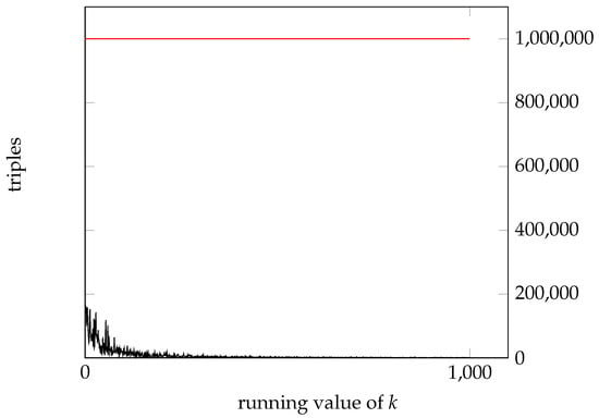
Figure 1.
Running Floyd–Warshall’s algorithm on a complete graph with vertices and random arc weights in . The bottom (black) plot shows the number of succeeding triples for increasing values of k, while the top (red) straight line shows, for each value of k, the number of tested triples, which is constant and equal to . The succeeding triples are a small fraction of the tested ones, and this fraction becomes smaller and smaller for increasing values of k. In the whole run, less than 1% of the tested triples lead to matrix updates, and most of them occur for low values of k, in the first part of the run.
In regard to the time performance of the Floyd–Warshall algorithm, the code states that each execution of testSP(i,j,k) requires a constant amount of time, say a, and each execution of updSP(i,j,k) requires a constant amount of time as well, say, b. Hence, the overall running time of the Floyd–Warshall algorithm is because . Indeed, Floyd–Warshall’s algorithm is very effective at performing a single iteration of the innermost loop, so the only chance to beat it is to reduce the number of evaluated triples without affecting the correctness of the result. The ideal case would be to only consider the triples belonging to , since any triple belonging to does not affect the matrix and, hence, the final result. However, precisely identifying appears to be a difficult task, for which there is no apparent faster solution than running Floyd–Warshall’s algorithm itself.
In this paper, we propose a heuristic strategy to identify a superset that, hopefully, is a close approximation of . Our experiments will show that, usually, has a much lower cardinality than . By running Floyd–Warshall’s algorithm over instead of , we increase the probability that a tested triple will succeed (i.e., the probability rises from to , and its value approaches 1 as becomes a good approximation of ). Notice that this strategy still produces the correct results, since by construction and Floyd–Warshall’s algorithm only needs to test the triples in to give the correct solutions (all other triples do not update the matrix). In order to identify , we are going to use a smart force approach.
The Smart Force Approach to All Pairs Shortest Paths
With respect to the determination of the successful triples in Floyd–Warshall’s procedure, we now describe and exploit a necessary condition that all successful triples must satisfy. We start by restating the general question asked within Floyd–Warshall’s algorithm in the body of the outermost loop (Lines 2 to 5 in Algorithm 1) as follows:
QFW: Given a current value for k, which pairs form a succeeding triple ?
Notice that there are n different values for k, and answering QFW for one value of k requires time with FW’s algorithm.
Let us now consider these two alternative questions:
Q1: Given current values for i and k, which indices j form a succeeding triple ?
Q2: Given current values for k and j, which indices i form a succeeding triple ?
Notice that finding the answers to Q1 and Q2 for all possible values of and would identify all succeeding triples; therefore, Q1 and Q2 together can be used to replace QFW. There are choices for both in Q1 and in Q2, but we aim to find each answer in less than time, thus realizing a speedup with respect to Floyd–Warshall.
The matrix value is updated if . Therefore, a necessary condition for a triple to succeed is
which we can rewrite as
When the pair is given, we check the first part of the condition over all j, and when the pair is given, we check the second part over all i. This way, all succeeding triples will be found, possibly in addition to some failing ones. The above checks are not done by complete enumeration (that would be a brute-force approach), but rather by direct access to the indices that can fulfill the stated necessary condition.
Let us consider the case of being fixed. The necessary condition for some j to be part of a succeeding triple with such i and k is that . For instance, this implies that if we knew that , then we could completely avoid the enumeration and testing of the n possible values for j when i and k are fixed to such values.
Therefore, we want to find only indices such that , . We find them by keeping a maxheap for each i, hosting all matrix values appearing in row i, with each value joined to its j index (we call it a row-heap because later we will need a similar column-heap, and the in stands for “row”). Using such a data structure, we can find the index associated with the maximum value in constant time, while fixing the heap after popping a value takes time. Finding the t (rather than n) triples requires time, which can be better than .
In a perfectly analogous way, when k and j are fixed, we keep n column-heaps , one for each j, and look for indices i such that .
Building the heaps at the very beginning costs per heap, for a total cost of . Each row-heap (and, respectively, column-heap) is implemented in the customary way as an array of n records , where represents a column- (respectively, row-) index, while is the value of an entry of (respectively, ). As an example, means that the highest value in row 3 is at column 5, and it is . Following the standard max-heap property, the second- and third-highest values of row 3 are in the next two entries of (not necessarily in this order). In general, each index h identifies a node of the heap whose left subtree is rooted at while its right subtree is rooted at .
While executing the algorithm, we need to keep the heaps consistent with L, i.e., each time an entry is updated, we must also update and . In order to make these updates effective, we use a back-pointer data structure for the heap, i.e., we keep “parallel” arrays (respectively, ) that indicate the position of each column index j (respectively, row index i) in the heap (respectively, ). In our example, since is the root of heap . This way, whenever is changed, we go to the node corresponding to j in and change its value (which necessarily decreases). In doing so, we let the node slide down in the heap by exchanging it with the largest of its two sons, if necessary, until it finds its correct position. We then record the new position of j in . The overall cost of this update is .
The main procedure for the version of the Floyd–Warshall algorithm based on the SmartForce technique (SF-FW) is outlined in Algorithm 2. We assume the input to be an cost matrix , and the final result, i.e., all-pairs shortest paths lengths, will be overwritten on .
| Algorithm 2 SF-FW |
1.
for
to
n
/*
create row-heaps
*/ 2. for
to
n 3. 4. 5. for
downto 1 6. heapify 7.
for
to
n
/*create column-heaps
*/ 8. for
to
n 9. 10. 11. for
downto 1 12. heapify;
13.
for
to
n 14. for
to
n
/*
run updates due to column k
*/ 15. 16. 0 17. while ( ) 18. popped[t] ← popHeapTop( ) 19. popped[t].ndx 20. popped[t].value eval 21. t++ 22. for
to
t
/*
restore heap
*/ 23. insertHeap( , popped[e] ) 24. for
to
n
/*
run updates due to row k
*/ 25. 26. 0 27. while ( .value ) 28. popped[t] ← popHeapTop( ) 29. popped[t].ndx 30. popped[t].value eval 31. t++ 32. for
to
t
/*
restore heap
*/ 33. insertHeap( , popped[e] ) |
The procedure starts by creating the row-heaps for each row i (lines 1–6) and column-heaps for each column j (lines 7–12). At the same time, the parallel arrays and are initialized within the procedure Heapify (Algorithm 3), which, while moving the elements in the heaps, keeps track of their positions.
| Algorithm 3 Heapify |
1. /* left son */ 2. /* right son */ 3. if
then
else
4. if
then
5. if
then 6. 7. 8. /*swap with the largest of its sons */ 9. |
The main loop starts at line 13, ends at line 33, and contains two sub-loops. The first one (lines 14–23) takes care of all the updates to due to the elements in column k, i.e., the pairs for varying i. A perfectly analogous loop (lines 24–33) concerns the updates due to row k of , i.e., pairs for varying j. We will comment only on the first loop since similar considerations hold for the second one.
The loop in lines 14–23 starts by determining the threshold , which must be beaten by an index j to be considered in a possibly succeeding triple. In lines 17–21, all heap elements such that are placed from the heap and put in a local buffer, . The triple is then evaluated and the new value of the entry is stored as the new value of X. At the end of the loop, t is the total number of elements that were popped, i.e., the total number of evaluated triples. At this point, the loop in lines 22–23 places the elements that were popped back into the heap with their new values. The back-pointers are updated within the procedure InsertHeap (Algorithm 4).
| Algorithm 4 InsertHeap |
1. H.SIZE++ 2. curr ← H.SIZE
3.
while
(curr > 1)
and
(H[].value < el.value) 4. Pos_H[ H[].ndx] ← curr 5. H[curr] ← H[] 6.
7.
Pos_H[el.ndx] ← curr 8. H[curr] ← el |
As far as the heap management is concerned, let us recall that a heap H is a binary tree stored in consecutive cells of an array (see [20]). We denote by the number of elements in a heap H, or, equivalently, the size of the array storing H. In general, the left son of node is node , while the right son of node is node . The max-heap property requires that the value of each node is not smaller than the value of any of its sons. Therefore, the largest value of any subtree is at the root node of the subtree.
Given an index v and an array of n records such that the subtrees rooted at and are heaps, the standard procedure Heapify (Algorithm 3) turns the subtree rooted at v into a heap. This is obtained by letting “slide” down in the heap until it finds its final position. This version of Heapify is such that the back-pointers to the heap are updated while the elements are moved around. Note that by calling Heapify for , an entire array can be turned into a heap.
The procedure InsertHeap (Algorithm 4) is used to insert a new element, say , into a heap H of less than n elements. The new element is initially put at the rightmost bottom leaf (position ) and then it is lifted to its final position, i.e., the position at which its value is no larger than its parent’s value. This is done with the loop in lines 3–6. The position of each element, which is moved down in the heap while moves up, is updated within the loop. Eventually, the element finds its final position in lines 7–8.
The procedure PopHeapTop (Algorithm 5) extracts from the heap H the element of maximum value (which is the root node, ) and returns it. It then rebuilds the heap by replacing the root with the leaf which, by calling , is moved down along the tree until the heap property is again fulfilled. The positions in the heap of the elements that are moved are updated accordingly, while the position of the element extracted from the heap is set to −1. Overall, the cost of the procedure is .
| Algorithm 5 PopHeapTop |
1. H[1].ndx, H[1].value⟩ /* get max element */ 2. Pos_H[k] ←−1 3. H[1] ← H[H.SIZE] /* overwrite it */ 4.
Pos_H[H[1].ndx] ← 1 5.
H.SIZE ← H.SIZE − 1 6. heapify(H,1) /* restore the heap */ 7. return |
3. Computational Experiments for the All-Pairs Shortest Paths Problem
All the computational experiments reported in this paper were run on an 11th Gen Intel® Core™ i7-1185G7 @3.00 GHz CPU with 16 GB RAM and a 64-bit operating system. We wrote the code in the C language and compiled it with the gcc compiler.
The cost of deciding which triple to test next is for the SF-FW procedure and for the unmodified Floyd–Warshall algorithm. Furthermore, the multiplicative constant that is embedded in the asymptotic notation for the time complexity of the SF-FW procedure is certainly higher than it is for the Floyd–Warshall algorithm. Finally, a drawback of the SF-FW procedure is that some triples might be evaluated twice, i.e., once because of and then again because of ]. This event, albeit rather unlikely, would happen when . Because of the reasons we just listed, the graphs on which we may expect SF-FW to outperform FW are those in which only a very small number of triples (compared to ) are updated during the execution of the Floyd–Warshall algorithm, and in which not many more than these are actually evaluated by SF-FW.
With these considerations in mind, let us analyze the algorithm’s behavior when running on some different types of graphs. In all our experiments, we used integer arc costs.
3.1. Graphs with “Few Updates”
As an extreme example, consider a complete graph where the arc costs are random numbers belonging to a range with . For such a graph, each arc is, in fact, the shortest path between its terminals; hence, no triple would lead to an update in the matrix.
As far as SF-FW is concerned, no entry is ever popped from the heaps for any target or , except during the phases in which or , i.e., when the target is one of the n diagonal elements of the matrix. In such cases, or, respectively, , and heap elements are popped. Therefore, only triples are checked for SF-FW while triples are checked for FW. Notice that the time needed to recognize that each arc is indeed a shortest path is , so SF-FW is optimal for this kind of graph.
If we slightly perturb this type of complete graph by altering “a few” entries, the SF-FW procedure outperforms Floyd–Warshall’s algorithm. For example, consider graphs with the described features, where we pick n arcs at random and give them a new random cost from , so that some triples will likely lead to an update (i.e., they are successful).
Table 1 reports the results for and , over graphs of nodes, with times in seconds. As can be seen, the SF-FW speedup factor over FW grows with n, with SF-FW being up to 15 times faster than FW for .

Table 1.
Results for complete graphs that need “very few updates”, with n “low cost” arcs, using and . Any table row reports data that has been averaged over 3 different random graphs, and the average numbers of triples are rounded to the nearest integer value. Time is reported in seconds.
To find the best field of application for SF-FW, we characterized classes of graphs that exhibit very few successful triples during the execution of the FW algorithm, thus yielding a very low ratio between successful and tested triples.
In such a way, the SF-FW procedure can handle a much smaller number of triples than the FW algorithm.
Let us consider complete graphs having some “easily reachable” vertices, called hubs. In such a graph, each arc incident on a hub is “short” (i.e., low cost), while all the other arcs may have any cost. As a real-life example, in road graphs, large cities connected by highways are quicker to reach than small, remote villages. A shortest path is most likely to use hubs as intermediate vertices. We assume that the hubs are the first nodes, say nodes . Indeed, if the hubs are processed first, then very few entries of the matrix will likely be updated in the following iterations of the algorithm. If we do not know which nodes are hubs, we could simply pre-process the input by sorting the vertices according to the average value of their incident arcs. This can be done in time .
In our experiments, we built complete graphs of this type according to the following parameters: is the number of hubs; m is the minimum cost for any arc; is the maximum cost for an arc incident on a hub; M is the maximum cost for any other arc. All arc costs are integers. We performed experiments with vertices and 5, 10, or 20 hubs. We set and M = 10,000 and varied the maximum cost of the arcs incident on the hubs in the set .
The results (with times in seconds) are reported in Table 2 and show speed improvements of up to 4× for the SF-FW procedure over the original Floyd–Warshall algorithm.
Table 2.
Comparison of FW and SF-FW on complete graphs with 5, 10, or 20 hubs, vertices, , M = 10,000, and . Time is reported in seconds. Any table cell reports data that has been averaged over 3 different random instances.
Of course, the computation time required by Floyd–Warshall’s algorithm is rather independent of the hub and arc costs, since most of the time spent is due to the exhaustive triple tests, which depend only on the number n of vertices in the graph (which is always 3000 for the whole table); very small variations arise from the number of updates that are executed.
As far as the SF-FW procedure is concerned, it achieves the best performance when the graph has a small number of hubs (five in this table) and when the costs of the arcs incident on hubs belong to a small range, [100, 120] in these experiments. The smaller the number of hubs and the smaller the cost range, the higher the speedup.
3.2. General Graphs and Range of Costs
When the arc costs vary over a large range (and, therefore, the lengths of the paths can also be very different), the overhead due to the heap management compared to the minimal bookkeeping of FW is such that the original FW can easily outperform SF-FW. However, when the arc costs belong to a smaller range, SF-FW becomes competitive and can eventually outperform Floyd–Warshall.
Table 3 reports experiments run on complete graphs with vertices, whose arc costs are drawn randomly from for various values of MAX. As can be seen, the SF-FW procedure benefits when the arc costs fall within a small range; for , SF-FW beats Floyd–Warshall for , but this range is probably too small to be really interesting. Let us note that gives only two possible values for costs, namely 1 or 2.
Table 3.
Results for complete graphs with vertices and random arc costs belonging to . Time is reported in seconds. Slow-downs are expressed as negative speedups. Each entry in the table reports data that has been averaged over 3 different random instances.
3.3. A Hybrid Approach
To make the SF-FW procedure effective even when the arc costs vary over a larger range than the graphs considered so far, we made the following observation. Typically, during the execution of Floyd–Warshall’s algorithm, the matrix values are updated many times in the early iterations, but once the values approach the correct shortest path lengths, it becomes increasingly difficult to improve them, and the number of updates drops dramatically (as shown in Section 2, Figure 1). Therefore, it appears sensible to begin with the original FW algorithm and use it for some iterations of the main loop, in order to exploit the effectiveness of FW during the many initial updates of the matrix cells, and then switch to the SF-FW procedure for the remaining iterations. We call this two-phase procedure a hybrid approach.
To test the hybrid approach and to calibrate the best switching point, we performed several experiments on complete graphs with various values of n and random arc costs drawn in the range . For each graph instance, we tested what would happen if we started with S iterations of FW followed by iterations of SF-FW, with and . Of course, when , the hybrid approach degenerates to SF-FW, while for it becomes FW.
From the results reported in Table 4, we can see that there is always a suitable switch point such that the corresponding version of the hybrid approach is better than FW. We highlighted (in boldface) the best switch point for each n, and it appears that, as n increases, the number of iterations of FW needed to achieve the best performance decreases. As a rule of thumb, we can also observe that, with the exception of , running initial FW iterations always yields better performance than both full FW and full SF-FW.
Table 4.
Results for the hybrid algorithm applied to complete graphs with random arc costs in the range . Time is reported in seconds. Any table cell reports data that has been averaged over 3 different random instances. The best switch point is highlighted (in bold) in each column.
Further experiments, reported in Table 5, were run to highlight the dependence of the best switch point on the width of the cost range, i.e., the value of MAX.
Table 5.
Results for the hybrid algorithm applied to complete graphs with vertices and random arc costs in the range . Time is reported in seconds. Any table cell reports data that has been averaged over 3 different random instances. The best switch point is highlighted (in bold) in each column.
The results, reported in Table 5, show that it is not easy to determine a fixed point at which to switch from FW’s original algorithm to SF-FWfor the remaining iterations. Indeed, calibrating the best switch point, either for specific instance classes or for generic random instances, appears to be an interesting and challenging question that might be the subject of future research.
In order to avoid the choice of a rigid threshold for the switching point, we also investigated the use of an adaptive threshold, as described in the following experiments. In this case, the main procedure decides the switching point at run time by estimating, through random sampling, the number of successful triples in the current iteration of the outermost loop. The rationale is that whenever we estimate that a large number of triples would fail in the current iteration (or within a suitable interval of consecutive iterations), then this would be a good time to switch to SF-FW.
Under this adaptive strategy, at each iteration of the FW outermost main loop (i.e., for each new value of k), a random sample of tested pairs is observed, say s pairs, giving a count of the successful ones. If , where p is a given threshold for the success probability, the hybrid algorithm switches from FW to SF-FW. Hence, this adaptive strategy is driven by two parameters—s and p—whose effects on the overall performance are investigated in the following table.
Table 6 reports the results for some experiments on various types of graphs, each of nodes. In order to make the switching decision more robust, we also introduced two extra parameters, named w and c. w indicates the size of a “window of consecutive iterations” considered when making the decision to switch or not to switch, while c, where , indicates how many times the switching condition must be satisfied, within the last w iterations, in order to switch to SF-FW. In particular, if , then the condition must be true for all the last w iterations in order to switch, while if , we switch as soon as the condition becomes true for the first time. It can be noted that, for this hybrid approach, there are several parameters to take into account, and the possible combinations of their values are too many to be considered fully in this first attempt, whose main goal is to present a new methodology. Indeed, the study of calibrating the best possible thresholds for a hybrid approach, either fixed or adaptive, will be the subject of future research. In the table, we just aim at showing a few examples of the effect of changing some parameters for some types of instances.
Table 6.
Complete graphs with . If , all graphs are clustered, and have , , and M = 10,000. Columns Floyd–Warshall and SF-FWreport the times (in seconds) of pure Floyd–Warshallãnd pure SF-FW, respectively. Column shows the best switching point, with the corresponding best time near it. The remaining columns describe the performance of the adaptive hybrid for the given parameters.
In these preliminary experiments, we first determined by enumeration the true best switching point, say , for each instance. represents the “goal,” i.e., the iteration at which we would have switched if we could have foreseen the future. We then ran the same instances with various values of p, s, c, and w to see how close the “adaptive” switching point, denoted , came to the best one and, more importantly, whether the hybrid performed better than Floyd–Warshall alone. From the table, we see that with , the hybrid algorithm switches at approximately the right time for graphs with hubs and performs much better than Floyd–Warshall alone. For instance, with no hubs and costs in { 10,000}, the hybrid is worse than FW for , while with a smaller p it degenerates into FW and, therefore, is not any worse. In graphs with costs in , we can see the effect of increasing the window size and requiring a significant amount of signal in order to switch, i.e., the condition is fulfilled 45 times in a row. Under these circumstances, the switching point is almost optimal, and the best improvement over FW is achieved.
4. The Transitive Closure Problem (TC)
Similar to the all-pairs shortest paths problem, a potential waste of time can be identified in Algorithm 6 (FW2), which computes the transitive closure of a graph. Inside the three nested loops of Algorithm 6 (FW2), the main instruction is an if test (in Line 4), which we call here testTC(i,j,k), whose conditionally executed body updates the content of one matrix cell, , by means of an assignment operation (in Line 5) that we call here updTC(i,j).
| Algorithm 6 FW2 |
1.
for
2. for 3. for 4. if then 5. ; |
In order to compute the transitive closure of a graph, Floyd–Warshall’s algorithm enumerates all the possible triples, executing the corresponding testTC(i,j,k), which, in turn, will cause the execution of some updTC(i,j), only when the test succeeds. Similar to Algorithm 1 (FW1), when a triple fails in Algorithm 6 (FW2), the time needed to perform the test is wasted. Clearly, the algorithm does not know in advance what triples will succeed; otherwise, only the succeeding triples would be enumerated, and the running time would improve. Let us recall here the condition tested by testTC(i,j,k):
where both and are Boolean values.
The main idea to avoid the check of failing triples is to know in advance which values of j, when paired with a given value of k, yield a true value for (similar considerations can be made on the knowledge of values of i that, together with k, yield = true). In this case, a given value of i will be considered for the evaluation of a triple only when paired with such values of j (and k). Note that these sets of values for j can be created in advance for any value of k.
For each possible value of k, let us call jset(k) the pre-built set of values of j such that = true. Analogously, let us call iset(k) the pre-built set of values of i such that = true. Then, Algorithm 6 (FW2) can be rewritten as Algorithm 7 (NewFW2):
| Algorithm 7 NewFW2 |
1. BuildJsets(T) /* shown later, a procedure */ 2. BuildIsets(T) /* shown later, a procedure */ 3.
for
4. foreach /* are pre-built sets */ 5. foreach /* are pre-built sets */ 6. ; /* no test needed: and are both true */ 7. add j to jset(i); 8. add i to iset(j); |
To complete the description, here are Algorithm 8 (BuildJsets) and Algorithm 9 (BuildIsets), used to pre-build the needed sets of indexes.
| Algorithm 8 BuildJsets (T) |
1.
for
2. jset(k) := new empty set 3. for 4. if then 5. add j to jset(k); |
| Algorithm 9 BuildIsets (T) |
1.
for
2. iset(k) := new empty set 3. for 4. if then 5. add i to iset(k); |
Such a modified Floyd–Warshall algorithm generates the same final matrix as the original algorithm (i.e., it finds the same correct transitive closure), without performing any test on the matrix values (i.e., it executes no if instruction) after the initialization phase, where the required sets are built. Of course, it needs to perform some set operations, in particular scanning the contents of sets (in the foreach loops) and adding elements to sets (in the pre-building phase and after any matrix update).
To stand a chance of outperforming the very fast Floyd–Warshall algorithm, we need a data structure that implements a set with very fast time performance for the needed operations, so we used a set implementation called FastSet [16] which offers optimal time performance for any set operation when the set elements are integer numbers (like in this problem). In particular, adding an element to a FastSet is and scanning a FastSet with cardinality c requires time. Hence, the new empty set operations in Line 2 of both Algorithm 8 and Algorithm 9 are actually new empty FastSet operations.
Of course, the pre-building phase is a time overhead for the whole new algorithm, even though it is , and the same holds for the (possible) addition of elements to sets after any matrix update. On the contrary, the new algorithm does not need to perform any if instructions inside the nested loops, so it saves some execution time. These two conflicting time behaviors give rise to an algorithm performance that is better than the original one in some interesting cases, as outlined in the next section.
As expected, the proposed algorithm beats the original one when the graph is very far from being complete (i.e., when it has a small number of arcs), because in such graphs the number of saved if instructions are large.
5. Computational Experiments for the TC Problem with FastSet
The first set of experiments, reported in Table 7, considers undirected random graphs of different sizes (i.e., different numbers of vertices) and different probabilities with which the arcs are drawn at random (e.g., when , the graph is complete, and when , there are no arcs). Clearly, there are no costs associated with the arcs in the transitive closure problem. Notice that the reported execution times for the proposed algorithm properly include the time needed to pre-build the sets of indices.
Table 7.
Random directed graphs with different percentages of arcs over all possible arcs (0% denotes a graph where all vertices are isolated, so the transitive closure matrix is completely filled by false Boolean values). Execution times (reported in seconds) have been averaged over 3 different random instances.
As far as the original Floyd–Warshall algorithm is concerned, its time performance with respect to is only affected by the number of successful triples, i.e., the number of matrix updates. Of course, the best case for such an algorithm is a graph with no arcs (), where all triples fail and no update is needed. The running time is still but the hidden constant is lower than in other cases since no execution of the update instructions will be performed. However, this particular case (i.e., when all triples fail) is also the situation in which our proposed algorithm has the best performance improvement over the original one, as can be seen in Table 7 by comparing the times reported in the columns labeled “0%”.
As soon as the value of increases, the execution time for the original algorithm increases as well, but the execution time for the new proposed algorithm increases even faster. We conclude that the proposed algorithm is very effective for sparse graphs, but not too suitable for dense graphs.
When the graph is undirected, the proposed algorithm can be slightly modified to obtain a significant time saving. In this case, both the cost matrix and the transitive closure are symmetric, and thus the algorithm does not need to compute and use both iset(k) and jset(k) sets. Indeed, since iset(k) = jset(k) for all values of k, one set of sets is enough. As can be seen in Table 8, when dealing with undirected graphs, the effectiveness of the proposed algorithm is much higher than for directed graphs.
Table 8.
Random undirected graphs with different percentages of arcs over all possible arcs. Execution times (reported in seconds) have been averaged over 3 different random instances.
The proposed algorithm is also effective at calculating the transitive closure for a different type of graph, namely cluster graphs (a cluster graph is the disjoint union of complete graphs). These experiments are reported in Table 9, where graphs with different numbers of clusters have been generated (of course, cluster graphs with only one cluster are complete graphs). As can be seen, both algorithms have better time performances on cluster graphs (the more clusters, the less time) than on graphs consisting of a single connected component, but the new algorithm benefits much more from clustering and, even with a few clusters (namely, five clusters in Table 9), it outperforms the original one.
Table 9.
Random undirected cluster graphs with the given number of components, each one being complete (please note that complete graphs as components are the worst case for the proposed algorithm). Execution times (reported in seconds) have been averaged over 3 different random instances.
Since the effectiveness of the proposed approach increases when the graphs (or their connected components) are more sparse, in Table 10 we report some experiments that just show what was expected, i.e., better time performances for graphs that are the union of disjoint sparse components (the more sparse the components, the better the performance). Of course, the last column of Table 10, labeled with 100%, is equal to the last column of Table 9, where complete components were considered.
Table 10.
Results of new TC-FW on random undirected graphs with 20 disjoint components, each one having the reported percentage of arcs over all possible arcs. Execution times (reported in seconds) have been averaged over 3 different random instances.
In the last experiment, we analyzed the performance of the proposed approach over an interesting class of graphs, namely the forests. A forest is a graph in which each connected component is a tree. Notice that trees are the most sparse among all possible connected components. Clearly, a forest with only one component is itself a tree. The results, reported in Table 11 and compared with Table 9, confirm that the proposed approach gains a great advantage from the graph sparseness.
Table 11.
Random forests with 1, 5, 10, and 20 components, with each component being a tree. Execution times (reported in seconds) have been averaged over 3 different random instances.
6. Conclusions
In this paper, we have undertaken the very challenging objective of improving one of the leanest and most effective graph algorithms, i.e., the triple-nested-for algorithm of Floyd and Warshall for the all-pairs shortest paths problem. By introducing and exploiting a necessary condition for the update of the matrix cells, and by using heaps in order to verify our condition in the most effective way, we have shown that the proposed algorithm can indeed supersede Floyd–Warshall’s algorithm on some interesting classes of graphs. Furthermore, we have presented evidence that the use of a hybrid, two-phase algorithm, which starts with FW and then switches to our proposed procedure, can in fact be more effective than Floyd–Warshall’s algorithm alone, even for general graphs. However, the best calibration of some parameters that can indicate when such a switch ought to be made requires further research and will be addressed in future work. Furthermore, we have studied how the same ideas used to improve FW’s algorithm for shortest paths could be applied to its algorithm for transitive closure computation. The main goal was to work only on the matrix cells that can change their value and avoid considering the others. By using FastSet to identify such cells, we have proposed a new algorithm that can be much quicker than the older one on sparse and/or non-connected graphs.
Author Contributions
Conceptualization: G.L.; both authors (G.L. and M.D.) contributed equally to the methodology, software, validation, formal analysis, data curation, and writing. All authors have read and agreed to the published version of the manuscript.
Funding
This research received no external funding.
Data Availability Statement
Data are contained within the article.
Conflicts of Interest
The authors declare no conflict of interest.
References
- Floyd, R.W. Algorithm 97: Shortest Path. Commun. ACM 1962, 5, 345. [Google Scholar] [CrossRef]
- Warshall, S. A theorem on Boolean matrices. J. ACM 1962, 9, 11–12. [Google Scholar] [CrossRef]
- Demetrescu, C.; Goldberg, A.V.; Johnson, D.S. (Eds.) The Shortest Path Problem: Ninth DIMACS Implementation Challenge; DIMACS Series in Discrete Mathematics and Theoretical Computer Science; American Mathematical Society: Providence, RI, USA, 2009; Volume 74, 319p. [Google Scholar]
- Yen, J.Y. Shortest Path Network Problems; Mathematical Systems in Economics; Hain: Nehren, Germany, 1975; Volume 18. [Google Scholar]
- Arranz, H.O.; Llanos, D.R.; Escribano, A.G. The Shortest-Path Problem: Analysis and Comparison of Methods, 1st ed.; Synthesis Lectures on Theoretical Computer Science; Springer: Berlin/Heidelberg, Germany, 2015; 87p. [Google Scholar]
- Edsger, W.; Dijkstra, E.W. A Note on Two Problems in Connection with Graphs; Numerische Mathematik; Springer: Berlin/Heidelberg, Germany, 1959; Volume 1, pp. 269–271. [Google Scholar]
- Bellman, R. On a Routing Problem. Q. Appl. Math. 1958, 16, 87–90. [Google Scholar] [CrossRef]
- Ford, L.R. Network Flow Theory; RAND Corporation Memorandum: Arlington, VA, USA, 1956; p. 923. [Google Scholar]
- Lawler, E.L. Combinatorial Optimization: Networks and Matroids; Holt, Rinehart, and Winston: Austin, TX, USA, 1976. [Google Scholar]
- Han, Y. An O(n3(loglogn/logn)5/4) time algorithm for all pairs shortest path. Algorithmica 2008, 51, 428–434. [Google Scholar] [CrossRef]
- Fredman, M.L. New bounds on the complexity of the shortest path problem. SIAM J. Comput. 1976, 5, 83–89. [Google Scholar] [CrossRef]
- Seidel, R. On the all-pairs-shortest-path problem in unweighted undirected graphs. J. Comput. Syst. Sci. 1995, 51, 400–403. [Google Scholar] [CrossRef]
- Lancia, G.; Rinaldi, F. New ideas to speed-up Floyd-Warshall shortest path algorithm. In Proceedings of the XLIX International Symposium on Operational Research SYM-OP-IS22 Proceedings, Vrnjacka Banja, Serbia, 19–22 September 2022. [Google Scholar]
- Brodnik, A.; Grgurovic, M.; Pozar, R. Modifications of the Floyd-Warshall algorithm with nearly quadratic expected-time. Ars Math. Contemp. 2022, 22, 1–22. [Google Scholar] [CrossRef]
- Sao, P.; Kannan, R.; Gera, P.; Vuduc, R. A Supernodal All-Pairs Shortest Path Algorithm. In Proceedings of the 25th ACM SIGPLAN Symposium on Principles and Practice of Parallel Programming, San Diego, CA, USA, 22–26 February 2020. [Google Scholar]
- Lancia, G.; Dalpasso, M. FASTSET: A Fast Data Structure for the Representation of Sets of Integers. Algorithms 2019, 12, 91. [Google Scholar] [CrossRef]
- Lancia, G.; Dalpasso, M. Finding the Best 3-OPT Move in Subcubic Time. Algorithms 2020, 13, 306. [Google Scholar] [CrossRef]
- Lancia, G.; Dalpasso, M. Algorithmic strategies for a fast exploration of the TSP 4-OPT neighborhood. J. Heuristics 2024, 30, 109–144. [Google Scholar] [CrossRef]
- Lancia, G.; Vidoni, P. Finding the largest triangle in a graph in expected quadratic time. Eur. Oper. Res. 2020, 286, 458–467. [Google Scholar] [CrossRef]
- Cormen, T.H.; Leiserson, C.E.; Rivest, R.L.; Stein, C. Introduction to Algorithms, 3rd ed.; The MIT Press: Cambridge, MA, USA, 2009. [Google Scholar]
Disclaimer/Publisher’s Note: The statements, opinions and data contained in all publications are solely those of the individual author(s) and contributor(s) and not of MDPI and/or the editor(s). MDPI and/or the editor(s) disclaim responsibility for any injury to people or property resulting from any ideas, methods, instructions or products referred to in the content. |
© 2025 by the authors. Licensee MDPI, Basel, Switzerland. This article is an open access article distributed under the terms and conditions of the Creative Commons Attribution (CC BY) license (https://creativecommons.org/licenses/by/4.0/).