Abstract
We primarily focus on the formulation, theoretical, and numerical analyses of a non-autonomous model for tuberculosis (TB) prevention and control programs in a population where individuals suffering from the double trouble of tuberculosis and diabetes are present. The model incorporates four time-dependent control functions, saturated treatment of non-infectious individuals harboring tuberculosis, and saturated incidence rate. Furthermore, the basic reproduction number of the autonomous form of the proposed optimal control mathematical model is calculated. Sensitivity indexes regarding the constant control parameters reveal that the proposed control and preventive measures will reduce the tuberculosis burden in the population. This study establishes that the combination of campaigns that teach people how the development of tuberculosis and diabetes can be prevented, a treatment strategy that provides saturated treatment to non-infectious individuals exposed to tuberculosis infections, and prompt effective treatment of individuals infected with tuberculosis disease is the optimal strategy to achieve zero TB by 2035.
Keywords:
saturated treatment; tuberculosis and diabetes mellitus co-dynamics; Pontryagin’s maximum principle; optimal control MSC:
92D25; 92D30; 49J15; 49N90
1. Introduction
Tuberculosis (TB) disease outbreak is a pandemic that is still present and its eradication has been a global health challenge for a long time [1,2,3]. It is an agelong respiratory illness. As noted by World Health Organization (WHO) in 2024, several years of progress achieved in the fight to end TB have been reversed because of the pandemic and countless other formidable challenges [4]; making TB the world’s deadliest infectious disease today, only second to the novel coronavirus during the pandemic in 2020. Subsequently, another report circulated by the Centers for Disease Control and Prevention (CDC) [5], in 2024, emphasized that there are still increasing TB incidences in the US.
Mycobacterium tuberculosis is a germ that causes tuberculosis infections. It is a pathogen that is ejected into the air when humans are sick with active tuberculosis disease and cough, talk, sing, or sneeze. When this airborne germ is inhaled by other humans, they contract tuberculosis in latent or active form depending on their immune response [6,7]. People with latent tuberculosis infections (LTBIs) are non-infectious and by the WHO’s estimate, around 1.7 billion people have LTBIs globally. If those exposed to the latent form of tuberculosis are not treated using the treatment regimen recommended by the WHO, preventing and controlling will be a difficult task since around 5 to 10 percent of the population exposed to TB would develop active TB in their lifetime [3].
Treatments are available for both inactive and active TB infections. Individuals hosting the sleeping bacteria in their bodies, i.e., latently infected persons, are administered some antibiotics by their healthcare providers, and this treatment regimen could last for three to four months [4,8]. Active TB disease can also be treated by several medications like isoniazid, rifabutin (Mycobutin), rifampin (Rimactane), pyrazinamide, ethambutol (Myambutol) and so on. Another way to ensure TB patients adhere to and comply with the treatment regimen is through Directly Observed Therapy, Short-course (DOTS) for TB infections [9]. This TB control strategy (DOTS for TB) was recommended by WHO towards the end of the 20th century and it is touted as the most proven, cost-effective tuberculosis treatment strategy [8]. Several countries have hence adopted DOTS for TB as a control measure towards TB prevention and control [4,9].
While tuberculosis is associated with poverty and its incidence is higher in poorer nations, noninsulin-dependent diabetes mellitus (NIDDM), alternatively named Type 2 diabetes, is a noncommunicable disease mostly common in rich nations in the past, but it is now prevalent in many TB-endemic, low- and middle-income countries (LMIC) [10,11,12]. NIDDM is also a global health threat and it happens due to insulin failure or the inability of the body to properly regulate the glucose in the blood plasma. Risk factors for NIDDM include obesity, poor diets, family history of diabetes, sedentary lifestyles, ethnicity, triglycerides (high cholesterol), non-alcoholic fatty liver disease, tuberculosis disease, etc. It has also been confirmed that there is a relationship between hyperglycemia (too much glucose present in the blood plasma) and the chronic complications, such as nephropathy (diabetic kidney disease), retinopathy, neuropathy, among people living with NIDDM [13,14].
There have also been reported cases of comorbidity of tuberculosis and other non-infectious diseases, particularly cardiovascular disease, cancer, noninsulin-dependent diabetes mellitus, etc. The bidirectional link between tuberculosis and noninsulin-dependent diabetes has been established through several research findings [3,12,14,15,16,17]. NIDDM is an increasing risk factor for tuberculosis disease as a result of immunodeficiency. People who are suffering from NIDDM with untreated tuberculosis infections in the latent form are at a greater risk of acquiring active tuberculosis disease due to weaker immune systems [3,14]. It is also a known fact that NIDDM is responsible for a high risk of treatment failure, mortality, and relapse among patients with active tuberculosis infections. Tuberculosis can also lead to glucose intolerance and severely affect glycemic control [18]. As of today, there is no known cure for NIDDM, but it can be well managed with patient education, healthy diets, lifestyle changes, expertise availability, medication, screening for complications associated with diabetes, proper glycemic control, and sustained observational follow-up [19,20].
The convergence, comorbidity, and concomitant conditions of tuberculosis and noninsulin-dependent diabetes mellitus have been presented in several epidemiological studies [7,12,14,17,21,22,23]. Moualeu et al. [12] developed and analyzed a compartmental TB model that assesses the impact of NIDDM in the spread of the tuberculosis disease in a community. Pan et al. [24] presented a mathematical modeling study on the effect of NIDDM on TB disease control in thirteen countries with a high burden of TB disease. Carvalho et al. [25] studied and assessed the role of diabetes in the progression of TB using a non-integer order model. Jajarmi et al. [26] used a fractional modeling approach to investigate the clinical implications of the comorbidity of tuberculosis and NIDDM. Moya et al. [27] examined the effectiveness of TB disease treatment therapy while taking into consideration the impact of associated diseases (NIDDM and HIV/AIDS). Awad et al. [28] used a mathematical modeling approach that utilized a recently developed age-structure NIDDM and TB co-infection dynamics to predict, estimate, and investigate the impact of noninsulin-dependent diabetes mellitus on mycobacterium tuberculosis epidemiology in Indonesia between 2020 and 2050. Agwu et al. [7] extended the study carried out in [12] by presenting the optimal control and some cost-effectiveness strategies for the mathematical model of TB and NIDDM co-infection dynamics. In [29], a deterministic mathematical model of the SEIS type that accounts for the saturated treatment of individuals exposed to mycobacterium TB in the latent form, along with crowding and psychological effects, was introduced to further study the impact of NIDDM in the transmission mechanism of TB in a community. Recently, Afolabi et al. [30] employ supervised machine learning algorithms to develop models that effectively predict diabetes from patients electronic health records (EHRs). For more detailed work on integer and non-integer compartmental models, see [31,32,33,34,35,36,37].
Over the years, several mathematical epidemiologists have developed and incorporated control strategies into disease models. Oke et al. [38] incorporated both pharmaceutical and non-pharmaceutical intervention strategies into a deterministic COVID-19 model used to garner insight into the transmission mechanism of the pandemic in the USA, South Africa, Italy, and Nigeria. Omede et al. [39] proposed and analyzed the autonomous and non-autonomous mathematical model of the third wave of the novel coronavirus in Nigeria. Olaniyi et al. [40] analyzed a malaria transmission model with protected travelers and partial immunity, where four preventive and control measures are implemented.
Following the lead of the aforementioned studies above, we formulate and analyze a non-autonomous deterministic model that evaluates the effect of the optimal treatment and prevention of the active and latent forms of tuberculosis infections among diabetic patients and nondiabetic individuals towards attaining the WHO’s global strategy to end the present TB epidemic by 2035. The remainder of this manuscript proceeds as follows: the autonomous form of the proposed non-autonomous model formulated in Section 2 is detailed in Section 3 and analyzed; Section 4 is dedicated to the theoretical analysis of non-autonomous mathematical model using the Pontryagin’s Maximum Principle; we illustrate the numerical simulation outputs of the several intervention strategies considered in this work in Section 5 and the last section summarizes our findings.
2. Non-Autonomous Mathematical Model System Formulation
This section is about formulating the optimal control model problem for the co-morbid association of noninsulin-dependent diabetes mellitus and tuberculosis. The model that we present here is a slight modification of the model for tuberculosis transmission proposed in [29], and it is its generalization. The optimal control’s primary goal is to identify the most effective approach to employ in the effort to eradicate TB in the population, that is, we want to derive optimal prevention and treatment strategies that come with minimal costs of implementation. Below are the definitions of the time-dependent controls that will be incorporated into the model that characterizes the dynamical transmission of mycobacterium TB disease in a human population compose of non-diabetic and diabetic individuals:
- (a)
- represents a TB prevention effort that screens for LTBIs among key groups of people in the population (i.e., people living with HIV or NIDDM, TB patients, family members, coworkers, and roommates) and promptly provides saturated treatment to those who have TB infections in the latent form. The cost of implementing this control includes identifying and screening key individuals who are at risk of being latently infected with tuberculosis, providing medications or directly observed treatment (DOT) to patients, and also non-death productivity losses by the patients.
- (b)
- is the tuberculosis and diabetes intervention to prevent people from developing either or both diseases. This is carried out through health and wellness promotions in the community, i.e., community awareness campaigns that encourage those diagnosed with pre-diabetes or gestational diabetes to go for routine screening with a diagnostic test for diabetes mellitus. Healthy diets and lifestyles advocacy. Prevention efforts towards developing complications are aimed at diabetic patients who are free of complications. Mass sensitization in the community on tuberculosis prevention. The cost of implementing this intervention strategy includes providing health education at home, hospitals, schools, and through mass and social media.
- (c)
- denotes TB control strategy that provides treatment to non-diabetic individuals suffering from active tuberculosis disease. The cost of implementing this control involves the amount spent on receiving treatment for tuberculosis by the patients, health care, allocation of resources for the treatment and management of people suffering from active tuberculosis infections and so on.
- (d)
- represents the TB treatment effort that caters to people living with tuberculosis and diabetes. The cost of implementing the control includes the expenses when receiving simultaneous treatment for tuberculosis and noninsulin-dependent diabetes mellitus, management of diabetic complications, health care workers, funding TB-NIDDM clinics, and so on.
The population is divided into nine categories where denotes the compartment of susceptible persons to both diabetes and TB, is the compartment for non-diabetic individuals exposed to tuberculosis, stands for the compartment of non-diabetic individuals infected with tuberculosis, is the compartment for diabetic individuals that do not develop complications, represents the compartment of individuals with diabetes without complications and exposed to tuberculosis, denote the compartment of actively infected individuals with tuberculosis and diabetic without complications, is the class of individuals with complications of NIDDM, denotes the compartment for individuals exposed to tuberculosis and have NIDDM with complications, and is the class of infected individuals with tuberculosis and have NIDDM with complications. For simplicity, we let ,
The following model assumptions are considered:
- The homogeneous mixing of individuals in the population and people in different classes interact.
- It is assumed that no individual in the population has permanent immunity to tuberculosis.
- The tuberculosis infection progression is from latency to the active disease stage, i.e., people first harbor tuberculosis infections in latent form and later become infectious either through exogenous reinfection or endogenous reactivation.
- We also assume the bidirectional link between tuberculosis and diabetes, i.e., diabetic patients can develop tuberculosis and tuberculosis patients can also become diabetic.
Hence, the non-autonomous model is as follows:
subject to the following initial conditions , , , with where
are saturated incidence rates first introduced by Capasso and Serio [41]. We assume that to take into account the increased infectiousness of people suffering from the comorbidity of complications of NIDDM and active tuberculosis disease [10,12]. We emphasize that without the controls (i.e., ), the model Equation (1) reduces to the autonomous compartmental model introduced in [29] with no saturated treatment of LTBIs and per-capita treatment of active TB. Refer to Table 1 for the biological definitions and values of the parameters used in model (1).

Table 1.
Model parameters, their definitions and numerical values.
We also let be the total human population. Suppose that From (1), it can be shown that
Assume that N is constant and (the recruitment rate) is positive, so, when the initial value is . Define the domain where the model is meaningful biologically below
Hence, in this work, the state variables and are restricted to the set . Let for . is a set (domain) such that it is positively invariant with respect to (1), that is, any solution that begins in stays there for all . Hence, the proposed optimal control mathematical model (1) is mathematically and epidemiologically (biologically insightful) well posed in the region .
Assume that for , are Lebesgue integrable and bounded control functions. Define a Lebesgue measurable control set by
Minimizing the total count of infectious and exposed individuals in the population and also the implementation costs of those intervention strategies ( and ) that are put in place is the objective of the optimal control technique. We propose the following objective functional J, defined as
is the elapsed time for the implementation of those control strategies, for represent the positive weight constants of both individuals exposed to and infected with TB, and denote the positive weight constants of for , the optimal controls. Note that quadratic treatment costs are assumed, that is, they are not linear in nature. Thus, we want to have and , the optimal control that satisfies
where is the Lebesgue measurable control set.
3. Analysis of the Mathematical Model with Constant Control Parameters
The four time-dependent control parameters, in this section, are considered as constants. We then find the equilibrium point (tuberculosis-free equilibrium), basic reproduction number, sensitivity analysis, and stability criteria for the model (1) where , and .
3.1. Equilibrium Points
The autonomous model (when we assume constant control parameters) will have the following tuberculosis-free equilibrium point
Hence, using the Next Generation Matrix approach [29,31,44,45], the basic reproduction number of the autonomous model is given below as
where
and , , , , , and . The following result on the local stability of the equilibrium point () was discussed in [29].
Theorem 1
([29]). The tuberculosis-free equilibrium point denoted by will be locally asymptotically stable if and unstable if .
It should be noted that Theorem 1 is a direct consequence of a theorem in [44] and its epidemiological significance is that tuberculosis disease will be under control in a case when the important threshold is below unity since a small number of people infected with tuberculosis in the population will not lead to a spike in new TB cases whenever
Theorem 2.
The partial derivatives of with respect to the constant control parameters and are negative.
Proof.
See Appendix A. □
By Theorem 2, we can conclude that increasing the constant controls and will result in a reduction in the value of the threshold parameter, , thereby helping in lowering the cases of tuberculosis in the population.
3.2. Sensitivity Analysis
Since the model system (1) with constant control parameters has a lot of parameters, we consider it imperative to perform the sensitivity analysis to know those parameters that contribute significantly to the transmission mechanism of TB in a population where people are either diabetes free or living with diabetes. We perform the local sensitivity analysis on the variable using the elastic index or normalized forward sensitivity index technique and the model parameter values in Table 1. We describe below the elastic index on with respect to a parameter :
Those parameters in Table 2 whose sensitive indices are negative (positive) will decrease (increase) the value of . It should be emphasized that the parameters and have a negative sensitivity index, and as a consequence, they will lower the value of , hence, they can be used as control parameters. If the values of the parameters, such as and with positive sensitivity, are decreased, the value of the reproduction number will also be decreased. For example, reducing each of the following parameters ( and ) values by 75%, the value of is reduced by 25.79%, 27.93%, and 48.40%, respectively. Also, if and are simultaneously decreased by (since , the basic reproduction number ( is decreased by 72.44%. This suggests that reducing the number of individuals with uncomplicated diabetes exposed to latent Mycobacterium tuberculosis (TB), preventing the development of uncomplicated diabetes, and controlling infectious TB among people with diabetes and its complications can significantly lower the community burden of TB. Furthermore, reducing the rate of TB transmission from infectious individuals living with the comorbidity of diabetes can help control the TB epidemic in a community. Finally, decreasing all the values of the five parameters and by 75% at the same time will give a corresponding reduction in the value of the basic reproduction number, such that It should be emphasized that the parameters and have negative sensitivity index, and as a consequence, will lower the value of , hence, they can be used as control parameters.
Table 2.
Sensitivity index of parameters of model system (1) with constant control parameters.
4. Theoretical Study of the Optimal Control Model Problem
Dynamic optimization is also a term for the theory of optimal control. This is a crucial tool in Mathematics, and is particularly used in decision-making that involves complex biological systems [46]. This section provides a detailed analysis of the non-autonomous, time-dependent TB-DM model (1). The approach we will take has been implemented extensively in several mathematical models that incorporate control strategies [7,37,38,39,40].
4.1. Existence of an Optimal Control
Theorem 3.
Suppose that , is the Lebesgue measurable admissible control set, , and denotes the right-hand side of (1) given by
Let for be the integrand of J, the objective functional, mentioned in (2). By Theorem 2.2 in [46], it is sufficient to prove the following properties to ensure that an optimal control exists:
(I) The permissible control set, U, is closed and convex.
(II) The boundedness of the state system by a linear function in both the control and state variables.
(III) For each , is convex in .
(IV) There exist positive constants and such that the Lagrangian is bounded below by
We establish properties (I)–(IV) as follows:
Proof.
See Appendix B. □
4.2. Characterization of the Optimal Control
Pontryagin’s maximum principle [47] is used in this section to establish the necessary conditions that an optimal control pair must meet. Now, if we use the principle, we see that (1) and (2) will be transformed into a problem whereby the Hamiltonian function, denoted by H, is minimized pointwise with respect to the following control variables , for Define the Hamiltonian H below:
where , and are the adjoint variables. The next result is the necessary conditions for the optimal control.
Theorem 4.
If there is an optimal control quadruple given by such that the objective functional, J, in (2), is minimized over the admissible control set U, and subject to the state system (1), then there are the adjoint variables satisfying the following adjoint system:
with transversality conditions
and
where
and
Proof.
We take the partial derivatives of the piecewise continuous Hamiltonian function, H, given by (6) with respect to each corresponding state variable to obtain the adjoint system stated in (7). By the Pontryagin maximum principle [47], there exist adjoint variables ( ) such that
with transversality conditions stated in (8).
Also, for us to obtain the optimal controls (9), we solve the following equations:
for ,
Lastly, using the standard control arguments involving the bounds on the control parameters, we then conclude that for
and for which
□
5. Numerical Simulations
The goal next is to execute the numerical simulations of the optimality system, which is comprised of the model system (1), and adjoint equations (co-state system) (7) with the following initial conditions ; along with the characterization of the optimal control (9), and transversality conditions (8) using the forward-backward sweep procedure in [46]. We choose the following weight constants , for the aim of demonstrating the optimal level of preventive and treatment strategies needed to minimize the number of people actively and latently infected with Mycobacterium TB.
The forward-backward sweep methods begin with initial guesses of for (control variables) and solve (1) and the non-autonomous state system in forward time by employing a Runge-Kutta iterative solver of order four accuracy. The adjoint (co-state) system (7) is then solved in reverse time with both iterative solutions of the state systems and the transversality constraints (8). We keep the admissible controls current by utilizing a convex combination of the controls that have been used previously and the characterization value.
Next, we will illustrate the impact of the control strategies that focus on the prevention of active TB/LTBI and Diabetes; the treatment of active cases of TB among diabetic and non-diabetic individuals and the prevention of the incidence of diabetes/TB and the prompt treatment of TB infections, either in the active or latent form. The baseline values of the model parameters in Table 1 were used for the simulations. The final time for implementing these control strategies is 10 years.
5.1. Intervention Strategy with Prevention of TB and Diabetes
Under this intervention strategy, the focus is mainly on preventing the populace from developing diabetes and tuberculosis infections in either the latent or active form. This preventive effort involves a treatment effort that provides a saturated treatment of TB infections in the latent form and mass sensitization of the community on how to prevent developing tuberculosis and diabetes. We use the control parameters and to minimize J, the objective functional (2), while . In Figure 1, we observe that TB disease persists in the infected classes () with or without the control strategy being executed (Figure 1a–c). At the end of the 10-year implementation period of this control strategy, only 1476 and 1082 TB infections were averted in the A and classes, respectively. We observe in Figure 1d,e that the number of people exposed to Mycobaterium TB in latent form in each L and compartments approach zero at the final time . The number of individuals latently infected with TB and diabetic (with its complications) decreased significantly with this control strategy and persists without control (Figure 1f).
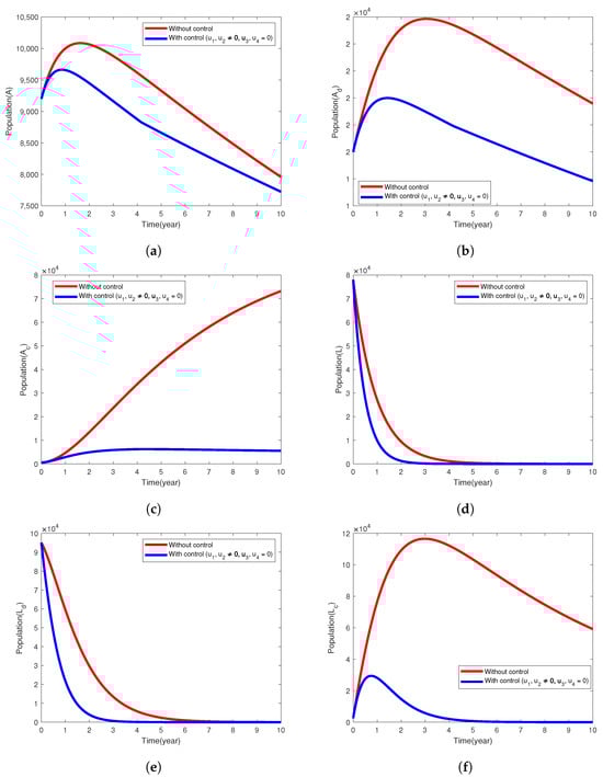
Figure 1.
Simulation results of the model (1) showing the variation in exposed and infected populations, the intervention strategy with prevention of active TB is implemented.
5.2. Intervention Strategy with Only Treatment of Active Cases of TB
Here, the control strategy involves the combination of treatment efforts of tuberculosis among diabetic and non-diabetic individuals, that is, the control variables and are used to minimize the objective functional, J. The simulation results in Figure 2a,b establish that this intervention strategy will significantly reduce the population of infected humans in A and compartments to two and eight people, respectively, at the end of executing this intervention strategy. The infected individuals in the class (Figure 2c) increased rapidly, and the mycobacterium TB disease is not under control, in fact, more than ten times its original population size, even with the implementation of this intervention strategy in place. The TB disease persists in all the infected classes and (Figure 2a–c) when the control variables are not used and also in the latently infected population with or without implementing the control strategy. We do not notice any clear difference in the populations of the exposed individuals () when the intervention strategy is used or not. It is observed that the individuals in the and L compartments decrease sharply at the end of 10 years (see Figure 2d–f).
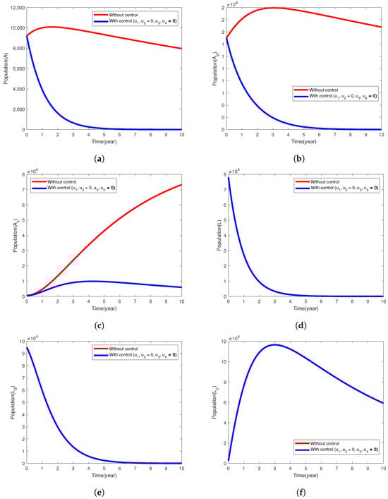
Figure 2.
Simulation results of the model (1) showing the variation in the exposed and infected populations when the intervention strategy with only treatment of active cases of TB is implemented.
5.3. Intervention Strategy with Prevention and Treatment
The control strategy combines all the control functions ( and ) and we assume they are nonzero, i.e., providing saturated treatment of latent tuberculosis infections (LTBIs), the treatment of infectious TB cases among diabetic and nondiabetic patients, and preventing the incidence of both diabetes and tuberculosis diseases. Figure 3 demonstrates how the implementation of all the control measures helps to control the spread of TB disease in the population. In Figure 3a–c, we see that the infected population A, and the latently infected populations approach zero at the end of the implementation period. The populations in the and compartments reduced considerably by 99.94%, 95.06% and 99.9%, respectively (Figure 3e,f). In the uncontrolled case, tuberculosis disease persists in all the following compartments (), and the population of latently infected individuals (L and ) declines sharply in 10 years.
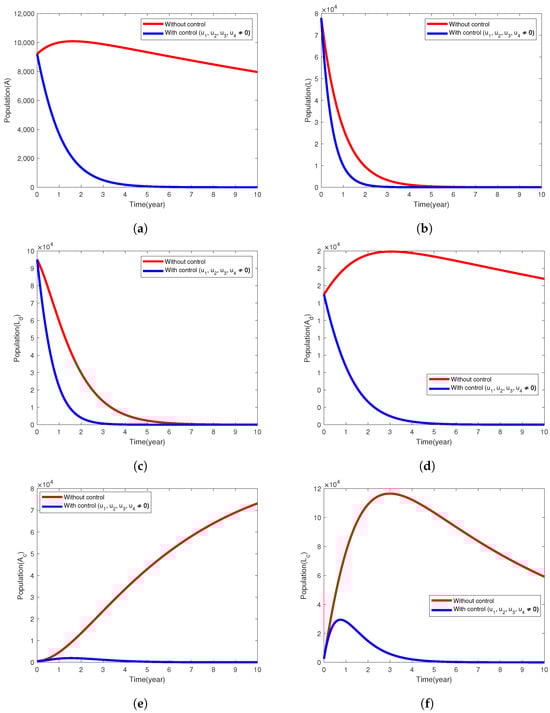
Figure 3.
Simulation results of the model (1) showing the variation in exposed and infected populations when the intervention strategy that combines all the control efforts is implemented.
In Figure 4, the optimal control profile graphs of different intervention strategies implemented are shown. It is observed that in the intervention strategy with the prevention of active TB and diabetes (Figure 4a), the control parameter should be sustained at the maximum bound throughout the control period and may be kept at the minimum level for the first 4 years and ought to be carried on at the highest bound throughout the rest of the implementation of this control strategy. For the intervention strategy with treatment effort towards active tuberculosis disease (Figure 4b), the control variables and should be maintained at the peak level for the implementation of this intervention strategy. Lastly, for the control strategy that combines all the control parameters, it is significant to mention that the control variable is to be upheld at the maximum bound throughout. and should sustain maximum efforts for 9 and 6 years, respectively. The control variable may be used at the lowest bound for the first 4.5 years and then should be maintained at its peak bound for the remaining years during the implementation period (see Figure 4c).
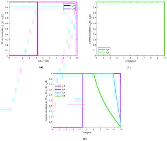
Figure 4.
Simulation results showing the profiles of the control functions used for each intervention strategy implemented.
6. Conclusions
The analysis of a non-autonomous (optimal control) mathematical model that captures the transmission mechanism of tuberculosis in a population where individuals are either diabetic or not was presented in this study. By taking the time-dependent control variables as constants, we compute (basic reproduction number), an important threshold in epidemiology, of the autonomous form of (1). Subsequently, the tuberculosis-free equilibrium point, , was established to be locally asymptotically stable whenever is below unity and unstable whenever exceeds unity. Through sensitivity indexes of the autonomous model parameters relative to , we justified the development of (1). Using the normalized forward sensitivity/elasticity index approach, those parameters that would have direct and indirect relationships with the future course of tuberculosis transmission in a population where some individuals are diabetic were identified. We further established that by reducing the rate at which people develop noncomplicated form of diabetes, rate (per-capita) at which noninfectious TB advances to active TB disease among those living with diabetes and its associated complications, and the modification parameter for increased rate of contracting active tuberculosis disease from those suffering from the double burden of tuberculosis and diabetes with/without complications, will result in a considerable decrease in the value of . Also, by increasing the time-independent control parameters and , the tuberculosis disease burden in the population will be diminished.
The analysis of the non-autonomous model (1) is built on the theory of optimal control. To find optimal intervention strategies for tuberculosis prevention and control, we considered the following four time-dependent functions which, in short, are the treatment efforts that screen for and diagnose LTBIs among key groups and immediately provide saturated treatment, preventive measures towards the development of either or both tuberculosis and diabetes diseases through community sensitization programs on radio, social media, television, etc., and the treatment efforts of infectious TB disease for people living with or without diabetes. We presented the theoretical analysis of the non-autonomous model problemand several simulation results of the four intervention (control) strategies considered in this work. It was noted that without the control strategies utilized, achieving control over the tuberculosis epidemic in the population will be a considerable challenge. The intervention strategy that has all four controls implemented is the optimal control strategy for preventing and controlling tuberculosis in the population, thereby, resulting in very few latent and active tuberculosis cases at the end of the implementation period of 10 years.
Author Contributions
Conceptualization, S.R.; Methodology, S.R., O.S.I. and S.I.O.; Software, S.R., O.S.I. and S.I.O.; Validation, S.I.O., O.S.I. and B.A.W.; Formal analysis, S.R.; Investigation, S.R., O.S.I. and B.A.W.; Data curation, S.R.; Writing—original draft, S.R.; Writing—review & editing, S.R., O.S.I., S.I.O. and B.A.W.; Visualization, S.R. and S.I.O.; Supervision, O.S.I. and B.A.W. All authors have read and agreed to the published version of the manuscript.
Funding
This research received no external funding.
Data Availability Statement
The Matlab codes employed to run the numerical experiments are available upon request to the authors.
Acknowledgments
We are grateful to the three anonymous reviewers and the handling editor for careful reading, constructive comments, and helpful suggestions, which have led to an improvement of the paper.
Conflicts of Interest
The authors declare that they have no conflicts of interest.
Appendix A. Proof of Theorem 2
Since it is clear that
where
Hence, . Following similar approach, it can easily be verified that and
Appendix B. Proof of Theorem 3
Since the control set , by definition, the closure condition in (I) is established. Also, suppose that and are any arbitrarily two points in U such that and . By applying the definition of a convex set provided in [46], we conclude that
∀, Hence, and that proves the convexity of U.
It should be noted that we can write in (5) as , such that
and
We follow the concept used in [40] to prove the boundedness of the state system. Then,
for some constants given by
where
That completes the proof of (II).
Therefore, it is sufficient to prove that is convex in , the control variable. We see that is a finite linear combination of the functions denoted by and for are positive coefficients. Now, we need to prove the convexity of the map defined by Also, as defined for a convex function in [46], choose and . Then,
Since , we have that Hence, the condition (III) is satisfied.
Finally, to verify the final condition (IV), we see that the Lagrangian given by
where
References
- abcNEWS, Kansas Faces One of the Largest Tuberculosis Outbreaks in Us History. Available online: https://abcnews.go.com/Health/kansas-faces-largest-tuberculosis-outbreak-us-history-health/story?id=118174420 (accessed on 30 January 2025).
- Orcau, À.; Caylà, J.A.; Martínez, J.A. Present epidemiology of tuberculosis. prevention and control programs. Enfermedades Infecc. Microbiol. Clin. 2011, 29, 2–7. [Google Scholar] [CrossRef] [PubMed]
- CDC. 2024 Tuberculosis (TB) Surveillance Report. Available online: https://www.cdc.gov/tb/risk-factors/diabetes.html (accessed on 21 May 2025).
- WHO. Global Tuberculosis Report 2024. Available online: https://www.who.int/teams/global-programme-on-tuberculosis-and-lung-health/tb-reports/global-tuberculosis-report-2024 (accessed on 21 May 2025).
- CDC, Provisional 2024 Tuberculosis Data, United States. Available online: https://www.cdc.gov/tb-data/2024-provisional/index.html (accessed on 21 May 2025).
- Cao, H.; Song, B.; Zhou, Y. Treatment strategies for the latent tuberculosis infections. J. Math. Biol. 2023, 86, 93. [Google Scholar] [CrossRef] [PubMed]
- Agwu, C.O.; Omame, A.; Inyama, S.C. Analysis of mathematical model of diabetes and tuberculosis co-infection. Int. J. Appl. Comput. Math. 2023, 9, 36. [Google Scholar] [CrossRef]
- Suárez, I.; Fünger, S.M.; Kröger, S.; Rademacher, J.; Fätkenheuer, G.; Rybniker, J. The diagnosis and treatment of tuberculosis. Dtsch. Aerzteblatt Int. 2019, 116, 729–735. [Google Scholar] [CrossRef]
- World Health Organization. Communicable Diseases Cluster. What is Dots?: A Guide to Understanding the Who-Recommended tb Control Strategy Known as Dots; Technical Report; World Health Organization: Geneva, Switzerland, 1999. [Google Scholar]
- Jeon, C.Y.; Murray, M.B. Diabetes mellitus increases the risk of active tuberculosis: A systematic review of 13 observational studies. PLoS Med. 2008, 5, e152. [Google Scholar]
- Krishna, S.; Jacob, J.J. Diabetes Mellitus and Tuberculosis, Endotext; MDText. com, Inc.: South Dartmouth, MA, USA, 2021. [Google Scholar]
- Moualeu, D.; Bowong, S.; Tewa, J.; Emvudu, Y. Analysis of the impact of diabetes on the dynamical transmission of tuberculosis. Math. Model. Nat. Phenom. 2012, 7, 117–146. [Google Scholar] [CrossRef]
- Tan, G.H.; Nelson, R.L. Pharmacologic treatment options for non-insulin-dependent diabetes mellitus. Mayo Clin. Proc. 1996, 71, 763–768. [Google Scholar] [CrossRef]
- Yorke, E.; Atiase, Y.; Akpalu, J.; Sarfo-Kantanka, O.; Boima, V.; Dey, I.D. The bidirectional relationship between tuberculosis and diabetes. Tuberc. Res. Treat. 2017, 2017, 1702578. [Google Scholar] [CrossRef]
- Bates, M.; Marais, B.J.; Zumla, A. Tuberculosis comorbidity with communicable and noncommunicable diseases. Cold Spring Harb. Perspect. Med. 2015, 5, a017889. [Google Scholar] [CrossRef]
- Vento, S.; Lanzafame, M. Tuberculosis and cancer: A complex and dangerous liaison. Lancet Oncol. 2011, 12, 520–522. [Google Scholar] [CrossRef]
- van Crevel, R.; Critchley, J.A. The interaction of diabetes and tuberculosis: Translating research to policy and practice. Trop. Med. Infect. Dis. 2021, 6, 8. [Google Scholar] [CrossRef]
- Nichols, G.P. Diabetes among young tuberculous patients, a review of the association of the two diseases. Am. Rev. Tuberc. Pulm. Dis. 1957, 76, 1016–1030. [Google Scholar]
- Garg, M.; Baliga, K. Management of type 2 diabetes (niddm). Med. J. 2002, 58, 53. [Google Scholar] [CrossRef][Green Version]
- Lefèbvre, P.J.; Scheen, A.J. Management of non-insulin-dependent diabetes mellitus. Drugs 1992, 44, 29–38. [Google Scholar] [CrossRef]
- Restrepo, B.I. Diabetes and Tuberculosis, Understanding the Host Immune Response Against Mycobacterium Tuberculosis Infection; Springer: Cham, Switzerland, 2018; pp. 1–21. [Google Scholar]
- Root, H.F. The association of diabetes and tuberculosis. New Engl. J. Med. 1934, 210, 127–147. [Google Scholar] [CrossRef]
- Alavi, S.M.; Khoshkhoy, M.M. Pulmonary tuberculosis and diabetes mellitus: Co-existence of both diseases in patients admitted in a teaching hospital in the southwest of iran. Casp. J. Intern. Med. 2012, 3, 421. [Google Scholar]
- Pan, S.-C.; Ku, C.-C.; Kao, D.; Ezzati, M.; Fang, C.-T.; Lin, H.-H. Effect of diabetes on tuberculosis control in 13 countries with high tuberculosis: A modelling study. Lancet Diabetes Endocrinol. 2015, 3, 323–330. [Google Scholar] [CrossRef] [PubMed]
- Carvalho, A.R.; Pinto, C.M. Non-integer order analysis of the impact of diabetes and resistant strains in a model for tb infection. Commun. Nonlinear Sci. Numer. Simul. 2018, 61, 104–126. [Google Scholar] [CrossRef]
- Jajarmi, A.; Ghanbari, B.; Baleanu, D. A new and efficient numerical method for the fractional modeling and optimal control of diabetes and tuberculosis co-existence. Chaos Interdiscip. J. Nonlinear Sci. 2019, 29, 093111. [Google Scholar] [CrossRef]
- Moya, E.D.; Pietrus, A.; Oliva, S.M. A mathematical model for the study of effectiveness in therapy in tuberculosis taking into account associated diseases. Contemp. Math. 2021, 2, 77–102. [Google Scholar]
- Awad, S.F.; Critchley, J.A.; Abu-Raddad, L.J. Impact of diabetes mellitus on tuberculosis epidemiology in indonesia: A mathematical modeling analysis. Tuberculosis 2022, 134, 102164. [Google Scholar] [CrossRef] [PubMed]
- Rasheed, S.; Iyiola, O.S.; Oke, S.I.; Wade, B.A. Exploring a mathematical model with saturated treatment for the co-dynamics of tuberculosis and diabetes. Mathematics 2024, 12, 3765. [Google Scholar] [CrossRef]
- Afolabi, S.; Ajadi, N.; Jimoh, A.; Adenekan, I. Predicting diabetes using supervised machine learning algorithms on e-health records. Inform. Health 2025, 2, 9–16. [Google Scholar] [CrossRef]
- Afolabi, Y.; Wade, B. Dynamics of transmission of a monkeypox epidemic in the presence of an imperfect vaccination. Results Appl. Math. 2023, 19, 100391. [Google Scholar] [CrossRef]
- Iyiola, O.; Oduro, B.; Akinyemi, L. Analysis and solutions of generalized chagas vectors re-infestation model of fractional order type. Chaos Solitons Fractals 2021, 145, 110797. [Google Scholar] [CrossRef]
- Brauer, F.; Castillo-Chavez, C. Mathematical Models in Population Biology and Epidemiology; Springer: New York, NY, USA, 2012. [Google Scholar]
- Blackwood, J.C.; Childs, L.M. An introduction to compartmental modeling for the budding infectious disease modeler. Lett. Biomath. 2018, 5, 195–221. [Google Scholar] [CrossRef]
- Iyiola, O.; Oduro, B.; Zabilowicz, T.; Iyiola, B.; Kenes, D. System of time fractional models for COVID-19: Modeling, analysis and solutions. Symmetry 2021, 13, 787. [Google Scholar] [CrossRef]
- Biala, T.A.; Afolabi, Y.O.; Khaliq, A. How efficient is contact tracing in mitigating the spread of COVID-19? A mathematical modeling approach. Appl. Math. Model. 2022, 103, 714–730. [Google Scholar] [CrossRef]
- Dere, Z.O.; Cogan, N.G.; Karamched, B.R. Optimal control strategies for mitigating antibiotic resistance: Integrating virus dynamics for enhanced intervention design. Math. Biosci. 2025, 386, 109464. [Google Scholar] [CrossRef]
- Oke, S.I.; Ekum, M.I.; Akintande, O.J.; Adeniyi, M.O.; Adekiya, T.A.; Achadu, O.J.; Matadi, M.B.; Iyiola, O.S.; Salawu, S.O. Optimal control of the coronavirus pandemic with both pharmaceutical and non-pharmaceutical interventions. Int. J. Dyn. Control 2023, 11, 2295–2319. [Google Scholar] [CrossRef]
- Omede, B.I.; Odionyenma, U.B.; Ibrahim, A.A.; Bolaji, B. Third wave of covid-19: Mathematical model with optimal control strategy for reducing the disease burden in nigeria. Int. J. Dyn. Control 2023, 11, 411–427. [Google Scholar] [CrossRef] [PubMed]
- Olaniyi, S.; Okosun, K.; Adesanya, S.; Lebelo, R. Modelling malaria dynamics with partial immunity and protected travellers: Optimal control and cost-effectiveness analysis. J. Biol. Dyn. 2020, 14, 90–115. [Google Scholar] [CrossRef] [PubMed]
- Capasso, V.; Serio, G. A generalization of the kermack-mckendrick deterministic epidemic model. Math. Biosci. 1978, 42, 43–61. [Google Scholar] [CrossRef]
- Mengistu, A.K.; Witbooi, P.J. Mathematical Analysis of tb Model with Vaccination and Saturated Incidence Rate; Wiley: Hoboken, NJ, USA, 2020. [Google Scholar]
- Egonmwan, A.O.; Okuonghae, D. Analysis of a mathematical model for tuberculosis with diagnosis. J. Appl. Math. Comput. 2019, 59, 129–162. [Google Scholar] [CrossRef]
- den Driessche, P.V.; Watmough, J. Reproduction numbers and sub-threshold endemic equilibria for compartmental models of disease transmission. Math. Biosci. 2002, 180, 29–48. [Google Scholar] [CrossRef]
- Baba, I.A.; Abdulkadir, R.A.; Esmaili, P. Analysis of tuberculosis model with saturated incidence rate and optimal control. Phys. A Stat. Mech. Its Appl. 2020, 540, 123237. [Google Scholar] [CrossRef]
- Lenhart, S.; Workman, J.T. Optimal Control Applied to Biological Models; CRC Press: Boca Raton, FL, USA, 2007. [Google Scholar]
- Pontryagin, L.S. Mathematical Theory of Optimal Processes; Routledge: New York, NY, USA, 2018. [Google Scholar]
Disclaimer/Publisher’s Note: The statements, opinions and data contained in all publications are solely those of the individual author(s) and contributor(s) and not of MDPI and/or the editor(s). MDPI and/or the editor(s) disclaim responsibility for any injury to people or property resulting from any ideas, methods, instructions or products referred to in the content. |
© 2025 by the authors. Licensee MDPI, Basel, Switzerland. This article is an open access article distributed under the terms and conditions of the Creative Commons Attribution (CC BY) license (https://creativecommons.org/licenses/by/4.0/).