Adam Algorithm with Step Adaptation

Abstract

Adam (Adaptive Moment Estimation) is a well-known algorithm for the first-order gradient-based optimization of stochastic objective functions, based on adaptive estimates of lower-order moments. As shown by computational experiments, with an increase in the degree of conditionality of the problem and in the presence of interference, Adam is prone to looping, which is associated with difficulties in step adjusting. In this paper, an algorithm for step adaptation for the Adam method is proposed. The principle of the step adaptation scheme used in the paper is based on reproducing the state in which the descent direction and the new gradient are found during one-dimensional descent. In the case of exact one-dimensional descent, the angle between these directions is right. In case of inexact descent, if the angle between the descent direction and the new gradient is obtuse, then the step is large and should be reduced; if the angle is acute, then the step is small and should be increased. For the experimental analysis of the new algorithm, test functions of a certain degree of conditionality with interference on the gradient and learning problems with mini-batches for calculating the gradient were used. As the computational experiment showed, in stochastic optimization problems, the proposed Adam modification with step adaptation turned out to be significantly more efficient than both the standard Adam algorithm and the other methods with step adaptation that are studied in the work.

1. Introduction

The ability to solve stochastic optimization problems is of key practical importance in many areas of science and technology such as energy management [1,2,3,4,5], healthcare [6], marketing [7] and various others.

Many problems in these areas can be represented as optimization problems of some objective function. If the function is differentiable with respect to its parameters, gradient descent, which does not use the values of the objective function, can become a relatively effective optimization method.

Often, the objective functions are stochastic. For example, many objective functions consist of a sum of subfunctions computed on different subsamples of the data. In this case, optimization can be more efficient by using gradient steps on individual subfunctions, such as stochastic gradient descent (SGD), which has played a key role in machine learning, particularly in deep learning [8,9,10,11,12]. Problems may also have other causes of noise. Such noisy problems require efficient stochastic optimization methods.

Adam [13] is an algorithm used for optimizing stochastic objective functions based on gradients. The method is simple to implement, computationally efficient, memory-efficient and well suited for both data-intensive and parameter-intensive problems. The method is also suitable for solving very noisy problems. Computational results show that Adam works well in practice [14,15].

Adam converges quickly in most scenarios, but sometimes it may not converge to an optimal solution, especially in cases with noisy or sparse gradients [16,17]. Tuning its hyperparameters can be critical to the model’s performance and is sometimes more sensitive than simpler optimizers. Additionally, for some problems, implementing annealing of the learning rate with Adam is necessary to achieve convergence, which adds another layer of complexity [18].

As we will see further, at a certain level of interference and degree of conditionality of the problem, the Adam algorithm is subject to looping. When solving applied problems, it is difficult to determine the reasons for the impossibility of obtaining a solution. This may be a defect caused by the algorithm or a defect caused by the formulation of the problem. Therefore, it is important to eliminate the defects generated by the lack of convergence of the algorithm.

Adaptive methods that adjust the step size have become widespread in large-scale optimization for their ability to converge robustly [19]. In [20], the authors proposed a method where each dimension has its own dynamic rate: large gradients have smaller learning rates and small gradients have large learning rates. The AdaGrad family of methods [16,21,22,23,24,25,26] is based on this principle and shows good results on large-scale learning problems. In [21], instead of accumulating the sum of squared gradients, the author fixed the window of past gradients that are accumulated. In [27,28], AdaGrad-Norm with a single step size adaptation based on the gradient norm was developed. Theoretical results for the advantage of AdaGrad-like step sizes over the plain stochastic gradient descent in the non-convex setting can be found in [29].

An adaptive optimization algorithm with gradient bias correction (AdaGC) was proposed in [30]. This algorithm improves the iterative direction through the gradient deviation and momentum, and the step size is adaptively revised using the second-order moment of gradient deviation.

In [31], AdaBelief is presented to adjust the step size according to the exponential moving average of the noisy gradient. If the observed gradient greatly deviates from the prediction, this method takes a small step; if the observed gradient is close to the prediction, the method takes a large step. AdaDerivative [32], in contrast to AdaBelief, can adaptively adjust step sizes by applying the exponential moving average of the derivative term using past gradient information without the smoothing parameter.

In [16], new variants of the Adam algorithm with a long-term memory of past gradients were proposed. The authors in [33] apply the variance reduction technique to construct the adaptive step size in Adam. The Cycle-Norm-Adam (CN-Adam) algorithm based on the cyclic exponential decay learning rate is proposed in [34]. Some well-known adaptive methods are shown in

Table 1. Some well-known adaptive methods.

Authors	Reference	Publication Years	Method
D.P.Kingma, J.P. Ba	[13]	2015	Adam
J.Duchi, E.Hazan, Y.Singer,	[20]	2011	AdaGrad
M.D.Zeiler	[21]	2012	AdaDelta
S.J.Reddi, S.Kale, S.Kumar	[16]	2018	AMSGrad
J.Chen et al.	[26]	2020	Padam
R.Ward, X.Wu, L.Bottou	[27]	2019	AdaGrad-Norm
Q.Wang et al.	[30]	2024	AdaGC
J.Zhuang et al.	[31]	2020	AdaBelief
W.Zou, Y.Xia, W.Cao	[32]	2023	AdaDerivative
L.Liu et al.	[33]	2020	RAdam
Shao, Y. et al.	[34]	2024	CN-Adam

.

The Adam algorithm has three main ideas: gradient smoothing, variable scaling and step selection. Our goal is to analyze the effectiveness of the degree of presence of these components in the minimization algorithm. In our proposed algorithms, the way to select the step multiplier was completely excluded.

In this paper, we present a method for tuning the step of the Adam method using the fact that in exact one-dimensional descent, the current descent direction is orthogonal to the gradient calculated at the new point. Based on observations of the angle between the current descent direction and the new gradient, the step will be tuned. If the angle is acute, the step is small and should be increased. If the angle is obtuse, the step is large and should be decreased.

The main property of the minimization algorithm is its convergence rate. It is known that with an increase in the degree of conditionality of the problem, the convergence rate of the gradient method decreases. We study the effect of the gradient noise on the convergence rate of the algorithm at a certain fixed level of conditionality that does not depend on the problem dimension. At the same level of conditionality for different dimensions, the convergence rate of the gradient method depends slightly on the dimension. As shown by our experiments, when moving, for example, from the dimension n = 100 to n = 1000, the methods under study show more stable results with respect to changes in the noise level. This allows us to conduct an extensive computational experiment with insignificant dimensions.

The proposed step adaptation procedure was applied to the Adam algorithm, momentum algorithm and gradient method. A computational experiment was conducted on functions with gradient noise, as well as on training problems with mini-batches for gradient calculation. As the computational experiment showed, the step adaptation algorithm allows eliminating loops inherent in the Adam method. The Adam algorithm with step adaptation, unlike other methods, managed to solve all test problems.

The rest of the paper is organized as follows. In Section 2, we give the problem statement and description of Adam algorithm. In Section 3, we consider principles of step adaptation and present the modified algorithms of Adam, momentum and the gradient method with step adaptation. In Section 4, we conduct a numerical experiment. Section 5 summarizes the work.

2. Problem Statement and Background

Let the problem of minimizing the function f(x), x ∈ Rⁿ be solved. In relaxation minimization methods, successive approximations are constructed using the formulas:

$$x_{k+1}=x_k-h_k{s}_k,s_k\in R^n.$$

(1)

Here, s_k is the descent direction, h_k is the step of one-dimensional (line) search, while f(x_k+1) ≤ f(x_k). These and other frequently used designations are given in

Table A1. Frequently used designations.

Designation	Meaning
gk,∇f	Gradient of a function
hk	Minimization step
hk*	Optimal value of minimization step
pk	Exponentially smoothed gradients
bk	Exponentially smoothed squares of gradients
sk	Descent direction
xk	Approximation of minimum
E	Mathematical expectation
${\beta }_1,{\beta }_2$	Exponential decay rates for the moment estimates
α	Stepsize parameter
ε	Small value
(a,b)	Scalar product for vectors a and b
a·b = a ʘ b	Hadamard product for vectors a and b
‖ ‖	Vector norm
r	Noise level
n_max	Maximum number of iterations

.

In exact one-dimensional descent

$$h_k=\arg \underset{h\in R}{\min }f(x_k-h{s}_k).$$

(2)

Denote the current gradient value by g_k = ∇f(x_k). In gradient noise conditions, smoothed gradient values are used:

$$p_k={\beta }_1{p}_{k-1}+\left(1-{\beta }_1\right)g_k,p_k\in R^n,{\beta }_1\in \left[0,1\right).$$

(3)

Previously, in [35,36], we proposed several algorithms for adapting the step of the gradient method without one-dimensional search. In this study, we extend the ideas of one of these algorithms to a number of gradient methods used for training neural networks. We consider algorithms in which space transformation is carried out using diagonal metric matrices, the diagonal elements of which we will store as a vector. Denote the Hadamard product for vectors a and b by a·b = a ʘ b. In the algorithms presented below, instead of matrices, scaling factors specified as a vector are used, for example, b_k ∈ Rⁿ. The descent direction in this case is calculated according to the following rule:

s_k = p_k ʘ b_k.

(4)

In what follows we will assume that we have the ability to calculate the gradient with noise and that the function value is unavailable. Thus, we do not have the ability to use one-dimensional search (2). In gradient algorithms in this case, various types of step multiplier settings are used.

Consider the Adam algorithm using the structure of the method with a metric space transformation, where a gradient and a transformed metric matrix are used to form the descent direction. In the Adam algorithm, exponentially smoothed gradients $p_k={\beta }_1{p}_{k-1}+\left(1-{\beta }_1\right)g_k$ are used as directions, the scales of which are changed by variables using exponentially smoothed squares of gradients $b_k={\beta }_2{b}_{k-1}+\left(1-{\beta }_2\right)g_k^2$. The metric matrix is diagonal and its main diagonal elements are formed based on exponentially smoothed squares of the gradient components. The next element is the method for forming a step along the descent direction.

In the algorithms presented below, the operations of multiplication, the division of vectors and raising them to a power will mean that there will be operations for the components of the vectors involved in the operation. The addition of a vector and a number will mean adding a number to each component of the vector. The initial values of the parameters in Algorithm 1 are chosen as in [13]. Let us consider the Adam algorithm.

Algorithm 1 (Adam)

1. Set β1, β2 ∈ [0, 1), ε > 0, step size α > 0, the initial point x0 ∈ Rn. The algorithm uses parameters β1 = 0.9, β2 = 0.999, ε = 10−8, α = 0.001. 2. Set k = 0, pk = 0, bk = 0, where pk, bk ∈ Rn. 3. Set k = k + 1, gk = ∇f(xk). 4. $p_k={\beta }_1{p}_{k-1}+\left(1-{\beta }_1\right)g_k$. 5. $b_k={\beta }_2{b}_{k-1}+\left(1-{\beta }_2\right)g_k^2$. 6. ${\widehat{p}}_k=p_k/\left(1-{\beta }_1^k\right)$. 7. ${\widehat{b}}_k=b_k/(1-{\beta }_2^k$). 8. Get the descent direction $s_k={\displaystyle \frac{{\widehat{p}}_k}{\sqrt{{\widehat{b}}_k}+\epsilon }}$. 9. Find a new approximation of the minimum $x_{k+1}=x_k-\alpha s_k$. 10. If the stopping criterion is met, then stop, else go to step 3.

Step 4 gives us the exponential average for the gradient. Step 5 gives us the exponential average for the squares of the gradient components. Steps 6, 7 and 8 form the descent direction. Steps 6, 7, 8 and 9 can be represented as follows:

$$s_k={\displaystyle \frac{p_k}{\sqrt{b_k}+{\epsilon }_1}},x_{k+1}=x_k-\alpha {\displaystyle \frac{\sqrt{1-{\beta }_2^k}}{(1-{\beta }_1^k)}}{s}_k$$

(5)

where first the descent direction is found and then the step multiplier is determined.

To assess the importance of the presence of the parameters p_k, b_k in the algorithm, we first use only p_k and then this together with b_k to organize the algorithm with step adaptation.

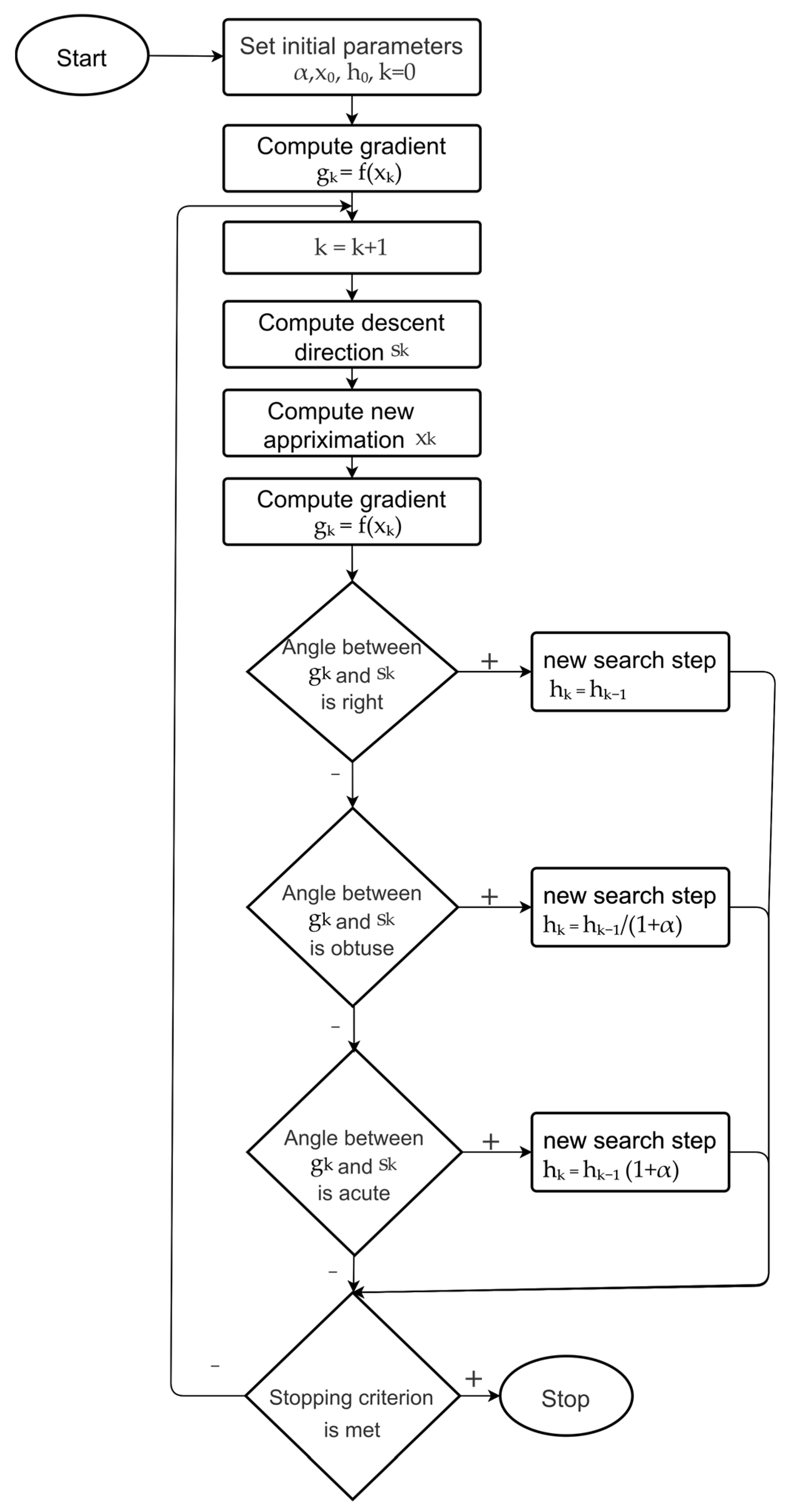
3. Algorithms with Step Adaptation

Consider gradient methods for minimizing a quadratic function

$$f_Q(x)={\displaystyle \frac{1}{2}}(x,Ax)-(b,x)+c,b,x\in R^n,A\in R^{n\times n}.$$

(6)

In the gradient method with a constant optimal step, the step size is determined by the expression

$$h^{*}=2/(M+m),$$

(7)

where M and m are the maximal and minimal eigenvalues of the matrix of second derivatives A. The estimate of the method (1) convergence rate for different ways of selecting the steps (2) and (7) is the same. To estimate step (2), the function derivative along the descent direction is used. The step is determined from the condition of the extremum of the one-dimensional function. The derivative at the optimal point must be zero.

Denoted by y(h) = −(∇f(x_k − hs_k), s_k), the derivative of function ϕ(h) = f(x_k − hs_k), with respect to the parameter h, can be computed in a minimization algorithm based on gradient information. If the function is quadratic, then y(h) is a linear function of h. In [35], the following estimate of the optimal step was obtained

$$h_k^{*}=h_k{\displaystyle \frac{y(0)}{y(0)-y(h_k)}}.$$

(8)

Estimate (8) is achieved only after obtaining a new point and calculating the gradient of it. To use estimate (8), the following reasoning is required. The gradient method with a constant step converges in a wide range of step size selection, but this range and the optimal step are fixed for a quadratic function, or for strongly convex functions with a Lipschitz gradient [37]. Therefore, in [35], estimate (8) is adopted as an estimate for step (7), towards which the current search step is moved. The simplest way to organize an algorithm of this kind is machine learning.

We form a quality functional

$$\Phi (h)=(h-h^{*})/2.$$

(9)

The gradient minimization method (9) at a certain step is

$$h_{k+1}=h_k-q_k{\Phi }^{\prime }(h_k)=h_k-q_k(h_k-h_k^{*}).$$

(10)

In [35], several methods of organizing update (10) were used. The most suitable for solving minimization problems under interference conditions was the following type of method:

$$h_{k+1}=h_k-q_{k}sign(h_k-h_k^{*}).$$

(11)

In (11), possible oscillations in values h_k − h_k^* are excluded.

Process (11) can be organized in another way. For this, we only need information about whether the step h_k value is greater or less than step h_k^*. Initially, the derivative is negative. In the case when the boundary of the zero value of the derivative is not reached and y(h_k) < 0, the step should be increased. When the boundary is passed, then y(h_k) > 0 and the step should be decreased. In this case, (11) is rewritten as

$$h_{k+1}=h_k-q_{k}sign(y(h_k)).$$

(12)

In [35], the following method of step adaptation in Algorithm 1 is used with q = (1 + α) > 1:

$$\begin{gathered} h_{k+1}=h_k{(1+\alpha )}^{-sign\left(y\left(h_k\right)\right)}=h_k{(1+\alpha )}^{sign\left(\nabla f\left(x_{k+1}\right),s_k\right)} \\ =\left\{\begin{array}{c}{h}_k\left(1+\alpha \right)if\left(\nabla f\left(x_{k+1}\right),s_k\right)>0,\\ h_{k}if\left(\nabla f\left(x_{k+1}\right),s_k\right)=0,\\ h_k/\left(1+\alpha \right)if\left(\nabla f\left(x_{k+1}\right),s_k\right)<0\end{array}\right., \end{gathered}$$

(13)

where we made the replacement y(h_k) = −(∇f(x_k − hs_k), s_k) = −(∇f(x_k+1), s_k).

In some cases, the following step adjustment may be effective:

$$h_{k+1}=h_k\left(1-\alpha ·sign\left(y\left(h_k\right)\right)\right)=h_k\left(1+\alpha ·sign\left(\nabla f\left(x_{k+1}\right),s_k\right)\right).$$

The step adaptation algorithm will be used to minimize functions with gradient interference. Therefore, for a random variable sign(y(h_k)) with E(sign(y(h_k))) = 0, we must have equality h_k+m = h_k for the same number of positive and negative values of sign(y(h_k)).

Update (13) ensures that the required equality h_k+m = h_k; that is, the absence of a trend component, with the same number of positive and negative values of sign(y(h_k)) on a segment of m updates.

In the case of high interference on the gradient, or essentially non-quadratic functions, instead of (1), we will use a process with the normalization of the descent vector

$$x_{k+1}=x_k-h_k{s}_k/\left|\right|s_k\left|\right|.$$

(14)

In the following Algorithm 2 (Figure 1), we use the gradient descent along the gradient g_k and step adaptation.

Algorithm 2 (H_GR)

1. Set the step adaptation parameter α > 0, the initial point x0 ∈ Rn and the initial step h0 ∈ R1. The algorithm uses parameter α = 0.01. 2. Set k = 0, compute gk = ∇f(xk). 3. Set k = k + 1. 4. Compute the descent direction. $s_k=g_{k-1}/‖g_{k-1}‖.$ 5. Find a new approximation of minimum $x_k=x_{k-1}-h_{k-1}{s}_k.$ 6. Compute gk = ∇f(xk). 7. Compute a new search step 7.1            If |(gk, sk)|≤ 10−15 then hk = hk−1 else 7.2                    If (gk, sk)≤ 0 then hk = hk−1/(1 + α) else 7.3                            hk = hk−1(1 + α). 8. If the stopping criterion is met, then stop, else go to step 3.

In Step 7, the step size of the method is adjusted. Condition 7.1 is necessary for cases where, due to noise or when calculating gradients based on mini-batches, the gradient vanishes. In 7.2, the step decrease is produced when the angle between s_k and g_k is obtuse. In 7.3, the step increase is produced when the angle between s_k and g_k is acute. The small value 10⁻¹⁵ in Steps 7.1–7.3 was chosen to exclude step adaptation at zero gradients.

The algorithm with a normalization of the descent direction is more stable when minimizing functions with interference and enables a wider range of the step adaptation algorithm parameter α in (13). Taking into account the variety of functions other than quadratic, where fluctuations in the gradient values can be significant, we will further use the algorithm (14) with step adaptation (13). Here, α is the adjustable parameter.

In the following Algorithm 3 (Figure 2), we use descent along the smooth gradient p_k and step adaptation to select the step.

Algorithm 3 (H_ MOMENTUM)

1. Set the exponential smoothing parameter β1 ∈ [0, 1), ε > 0, step adaptation parameter α > 0, the initial point x0 ∈ Rn and the initial step h0 ∈ R1. The algorithm uses parameters β1 = 0.9, ε = 10−8, α = 0.01. 2. Set k = 0, pk = 0, bk = 0, where pk, bk ∈ Rn, compute gk = ∇f(xk). 3. Set k = k + 1. 4. Compute $p_k={\beta }_1{p}_{k-1}+\left(1-{\beta }_1\right)g_{k-1}.$ 5. Find a descent direction $s_k=p_{k-1}/‖p_{k-1}‖$. 6. Find a new approximation of minimum $x_k=x_{k-1}-h_{k-1}{s}_k.$ 7. Compute gk = ∇f(xk). 8. Compute a new search step 8.1            If |(gk, sk)| ≤ 10−15 then hk = hk−1 else 8.2                  If (gk, sk) ≤ 0 then hk = hk−1/(1 + α) else 8.3                           hk = hk−1(1 + α). 9. If the stopping criterion is met, then stop, else go to step 3.

In Step 8, the step size of the method is adjusted. Using this algorithm, we will verify the efficiency of space metric transformation for the Adam algorithm.

In the Adam algorithm with step adaptation (Algorithm 4), we use components p_k and b_k together to form the descent direction. We called this algorithm Adam with step adaptation, although, to be completely precise, it is Adagrad with elements of momentum and step adaptation.

$$s_k={\displaystyle \frac{p_k}{\sqrt{b_k}+{\epsilon }_1}}.$$

(15)

Algorithm 4 (H_ADAM)

1. Set β1, β2 ∈ [0, 1), ε > 0, step adaptation parameter α > 0, the initial point x0 ∈ Rn, the initial step h0 ∈ R1. The algorithm uses parameters β1 = 0.9, β2 = 0.999, ε = 10−8, α = 0.01. 2. Set k = 0, pk = 0, bk = 0, where pk, bk ∈ Rn. Compute gk = ∇f(xk). 3. Set k = k + 1. 4. $p_k={\beta }_1{p}_{k-1}+\left(1-{\beta }_1\right)g_{k-1}$. 5. $b_k={\beta }_2{b}_{k-1}+\left(1-{\beta }_2\right)g_{k-1}^2$. 6. Get the descent direction ${\widehat{s}}_k={\displaystyle \frac{p_k}{\sqrt{b_k}+\epsilon }},s_k={\widehat{s}}_k/\parallel {\widehat{s}}_k\parallel$. 7. Find a new approximation of the minimum $x_k=x_{k-1}-h_{k-1}{s}_k$. 8. Compute gk = ∇f(xk). 9. Compute a new search step 9.1          If |(gk, sk)| ≤ 10−15 then hk = hk−1 else 9.2               If (gk, sk) ≤ 0 then hk = hk−1/(1 + α) else 9.3                     hk = hk−1(1 + α). 10. If the stopping criterion is met, then stop, else go to step 3.

The required moving averages are calculated in Steps 4 and 5. The descent direction is calculated based on the components p_k, b_k and normalized in Step 6. The meaning of the adaptation step in Step 9 is the same as for Algorithm 2.

By varying the parameters of exponential smoothing β₁, β₂ ∈ [0, 1), we can study the effect of gradient and gradient squares smoothing on the efficiency of the minimization. As a result of the computational experiment, it was found that the parameter values β₁ = 0.9 and β₂ = 0.999 were the best for complex situations, with both large noise or with small mini-batches for calculating the gradient.

4. Numerical Results and Discussion

The goal of the numerical experiment is to experimentally study the ability of methods to maintain operability under interference conditions. The use of multi-step gradient methods is justified primarily on ill-conditioned functions that are difficult to minimize using the gradient method. Test functions are selected based on this position. Some functions differ significantly from quadratic ones and contain curvilinear ravines, which reflects the situation of rapidly changing eigenvectors of the matrix of second derivatives.

The local convergence rate of the gradient method in a certain neighborhood of the current minimum is largely determined by how effective it is in minimizing ill-conditioned quadratic functions. Therefore, testing was primarily carried out on quadratic functions, where it is easy to control the degree of conditionality of the problem.

Testing is performed on smooth test functions. The minimum of test functions is uniquely defined. Test functions include functions with curvilinear ravines and functions that differ significantly in properties from quadratic ones. The well-known Adam algorithm and algorithms with step adaptation were chosen as the algorithms under study: H_GR—gradient method with step adaptation, H_MOMENTUM—momentum method with step adaptation and H_ADAM—Adam algorithm with step adaptation. The Delphi 7 software environment was used to implement the algorithms.

For test functions, we use the notation f(x,[parameters]). In calculations, we use the gradient of the function with noise $\nabla f_r=\nabla f+r\left|\left|\nabla f\right|\right|V$, where V is a random vector uniformly distributed in the unit sphere and the value of r varies. A higher value of parameter r means higher noise.

All the methods under study use only gradient values. The function values are calculated for the purpose of assessing the method’s progress in function minimizing and as a stopping criterion. The stopping criterion is

$$f(x_k)-f*\le \epsilon .$$

(16)

The initial point x₀ and the ε value are given in the description of the corresponding function. To solve the problem, for each function, the algorithm has a given number of iterations, n_max, if the stopping criterion is not met.

The result tables for each function indicate the number of algorithm iterations required to achieve the specified accuracy. If the algorithm does not achieve the specified accuracy in the allotted number of iterations n_max, then only the achieved function value is indicated underlined.

4.1. Preliminary Analysis of Algorithm Parameters

When solving an optimization problem, it is important to evaluate the ability of the algorithm to maintain its inherent convergence rate on functions with a given degree of problem conditionality. For these purposes, we will conduct a preliminary analysis of the method’s convergence rate under deep optimization conditions in order to analyze its descent trajectory. We carry this out by setting a stopping criterion corresponding to deep optimization and a significant number of iterations for monitoring the optimization process, which is set as one of the stopping criteria.

In [35], a quadratic growth of the number of iterations is shown depending on the ratio of the noise value to the gradient norm. In order to be sure that the algorithm actually converges not by chance and to verify the method convergence under noise conditions, we also need to set a deep optimization criterion and perform the required number of iterations, which can be very large. Such statistics will allow us to obtain an idea of the non-random nature of the algorithm convergence. Thus, with stopping criteria that ensure deep optimization, we obtain information on the algorithm behavior over a significant segment of the function decrease.

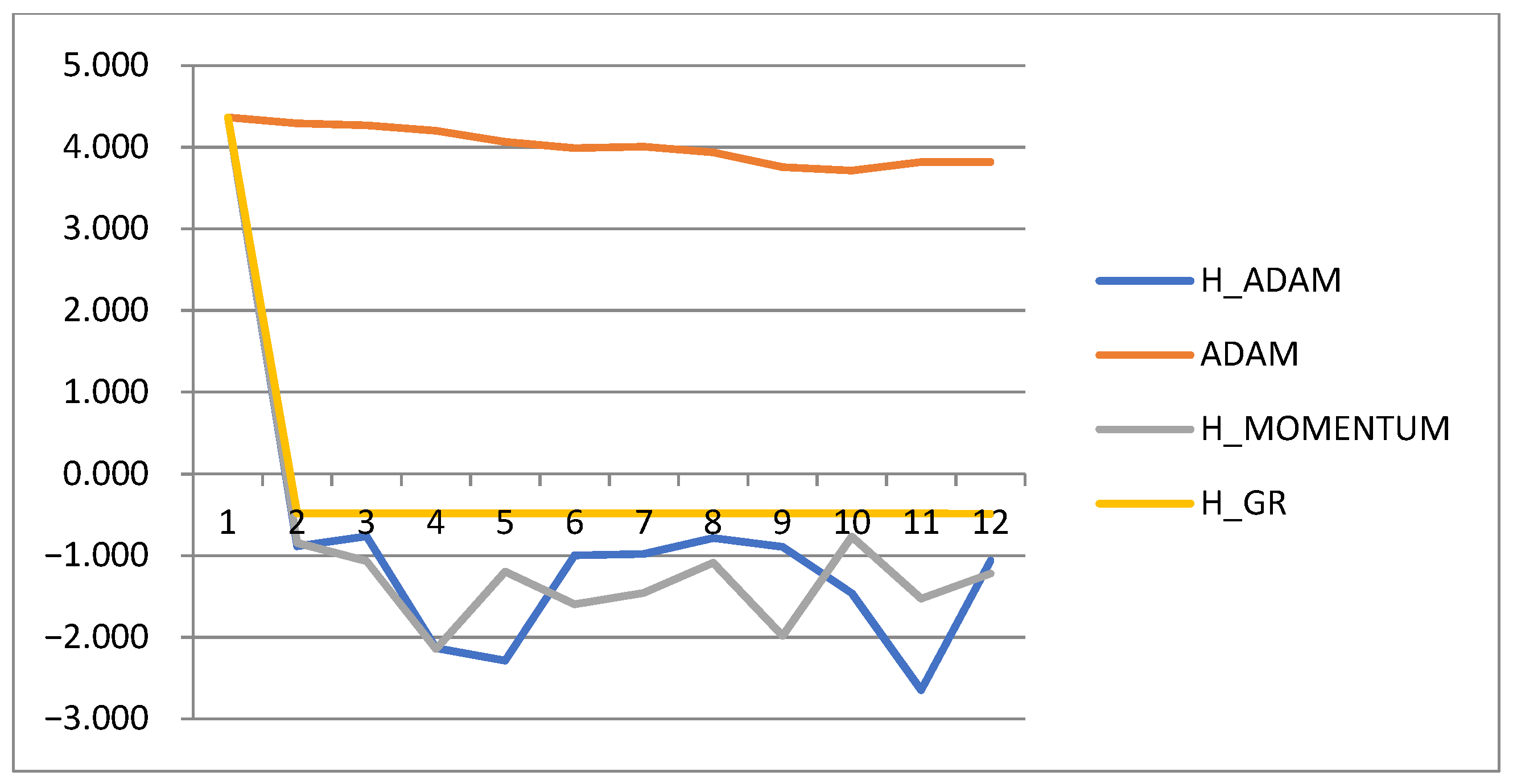
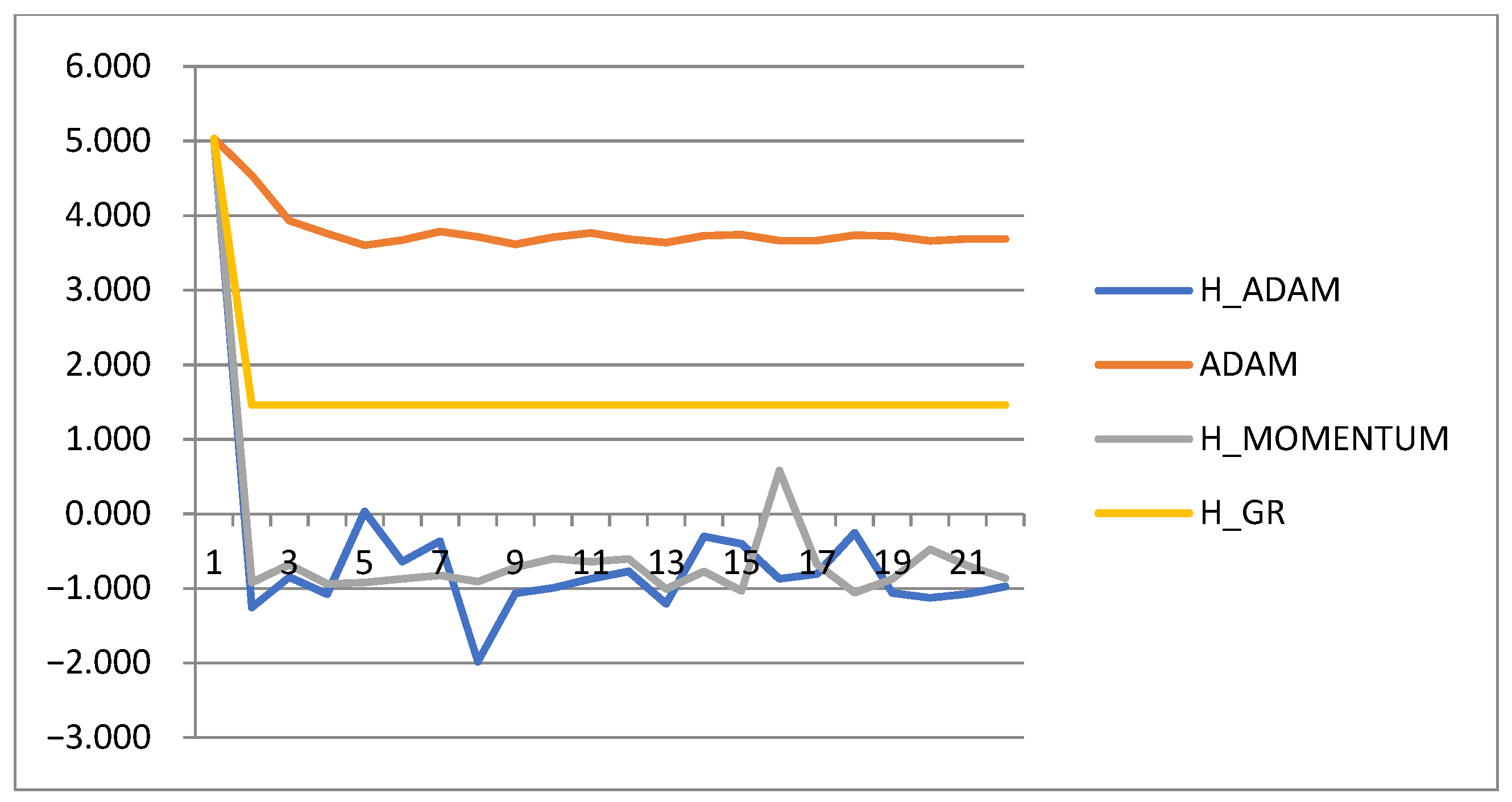
4.1.1. Convergence Rate Analysis

We conduct an experiment on the following function:

$$f_Q(x,[a\max ])={\displaystyle \frac{1}{2}}{\displaystyle \sum _{i=1}^n{a}_i{x}_i^2},a_i=a{\max }^{{\displaystyle \frac{i-1}{n-1}}}.$$

Eigenvalue a_i of this function has the boundaries λ_min = 1 and λ_max = a_max. Increasing the a_max value leads to an increase of problem conditioning. The initial points are x₀ = (100, 100, …, 100), n = 100, n_max = 100,000. The parameters are β₁ = 0.9, β₂ = 0.999 and α = 0.01.

Table 2. Number of iterations for the f_Q(x,[a_max]) function minimization depending on the a_max.

amax	$\mathit{f}\left({\mathit{x}}_{\mathit{k}}\right)-\mathit{f}*\le {10}^{-4}$				$\mathit{f}\left({\mathit{x}}_{\mathit{k}}\right)-\mathit{f}*\le {10}^{-10}$
	ADAM	H_GR	H_MOMENTUM	H_ADAM	ADAM	H_GR	H_MOMENTUM	H_ADAM
10	5307	216	489	607	5307	944	79,147	12,679
102	5307	720	418	5143	5307	1407	60,540	11,498
103	5307	4451	854	4167	5307	7892	1243	4917
104	5307	44,442	2205	891	5307	78,882	3892	1572

shows the results of minimization with different values of stopping criterion.

The H_GR algorithm most accurately reflects the dependence of the method on the degree of the problem conditioning. With a certain selection of the gradient smoothing parameter β₁, the other methods will also show an increasing number of iterations as the conditionality worsens. Such a selection should be carried out for the class of applied problems.

For the function f_Q(x,[a_max = 10⁴]) from Table 2, the trajectory of the function decrease for all the studied methods on a logarithmic scale is shown in Figure 3.

All step-adaptive methods converge linearly on each section of the trajectory. Since we did not obtain complete information about the convergence of the ADAM algorithm with the number of iterations of 100,000, we will conduct an experiment with a doubled number of iterations (Figure 4).

For the ADAM method, the trajectory has a very small segment of high convergence rate. From Figure 3 and Figure 4, we can draw the following conclusions. For step-adaptive methods, the convergence rate is constant along the descent trajectory. The ADAM method has three possible situations. If the step is small then the convergence rate is low, which we observe in the first data segment. If the step is optimal, then the speed is high. If the step is large, then oscillations occur in the minimum neighborhood. Based on the findings, it is necessary to choose the optimal step size for the ADAM method while a narrow range of its high efficiency exists. The graphs can be used to track the required level of criterion optimization, for example, 10⁻⁴.

Our goal is to identify defects in the convergence rate of methods. Comparing the results for the H_ADAM and ADAM methods in Table 2, we can note a sharp deterioration in their convergence rate with increasing optimization accuracy. It is especially important to set overestimated optimization criteria when minimizing functions with noise. In [35], a quadratic increase in the number of iterations is shown depending on the ratio of the noise value to the gradient norm. For example, with a tenfold noise increase, the cost of the number of iterations increases by 100 times. In order to verify the convergence of the method under noise conditions, we also need to set a deep optimization criterion and perform a large number of iterations. Such statistics will allow us to obtain an idea of the non-random nature of the algorithm convergence. Therefore, in the tests below, the stopping criteria will be set to a high degree of accuracy with large stopping values for the number of iterations.

4.1.2. Analysis of Step Adaptation Parameter

For the function f_Q, we will conduct a sensitivity analysis for the step adaptation parameter α; the results are presented in

Table 3. Number of iterations for the f_Q(x, [a_max]) function minimization depending on the α.

α	amax = 104, n_max = 200,000				amax = 10, n_max = 100,000
	ADAM	H_GR	H_MOMENTUM	H_ADAM	ADAM	H_GR	H_MOMENTUM	H_ADAM
0.1	2253 × 10−5	78,107	5835	2804	109,253	169	359	343
0.01	2253 × 10−5	78,882	3892	1572	109,253	944	79,147	12,679
0.001	2253 × 10−5	78,889	15,769	17,992	109,253	3011	12,475	19,522

.

The value of the parameter α determines the rate of the step change. For complex problems, it should be decreased (α = 0.001); on the contrary, for simple problems, it should be increased (α = 0.1). This thesis is confirmed by the results of Table 3. For a more complex problem, α = 0.01 is better. For a simpler problem, α = 0.1 is more suitable.

4.1.3. Analysis of Exponential Smoothing Parameters

For the function f_Q, we will conduct a sensitivity analysis for the parameter β₂, which is responsible for smoothing squares of gradient components. The parameters α = 0.01, n_max = 200,000 were set. The results are presented in

Table 4. Number of iterations for the f_Q(x, [a_max = 10]) function minimization depending on the parameter β₂.

β2	ADAM	H_ADAM
0.3	1901 × 10−2	1934
0.5	1063 × 10−3	1684
0.7	1379 × 10−4	1533
0.9	6094 × 10−5	1502
0.999	2253 × 10−5	1572

.

The analysis shows that, here, the best value for ADAM is β₂ = 0.999, and for H_ADAM, it is β₂ = 0.9. In general, it is recommended in the original ADAM to set β₂ = 0.999. Therefore, all experiments with the ADAM and H_ADAM algorithms are carried out with this value. In the example of this problem, there are no big differences in the behavior of the algorithms with β₂ = 0.999 and β₂ = 0.9. Nevertheless, this parameter can be selected for a set of similar problems.

There is also an optimum for the β₁ parameter, but the dependence of the parameter β₁ on the degree of degeneracy of the function follows from a comparison of the gradient method (β₁ = 0) and other methods. It is obvious that this parameter should be reduced as the conditionality of the function decreases.

4.2. Test Functions

4.2.1. Rosenbrock Function

The Rosenbrock function has the following form:

$$f_R(x)=100{(x_2-x_1^2)}^2+{(x_1-1)}^2.$$

(17)

The initial point is x₀ = (−1.2, 1) and the minimum point is x^* = (1, 1), ε = 10⁻¹⁰, n_max = 1,000,000. Note that the Rosenbrock function is not convex.

Table 5. Number of iterations for the Rosenbrock function minimization with gradient interference.

r	ADAM	H_GR	H_MOMENTUM	H_ADAM
0	12,315	11,252	2094	10,001
1	13,721	11,269	7140	11,021
2	116,779	31,477	18,938	18,921
3	44,111	29,050	38,862	41,404
4	260,210	147,051	1064	148,752
5	934,950	168,840	112,545	112,284
6	1301 × 10−5	429,597	83,790	80,820
7	2872 × 10−4	571,974	152,464	182,693
8	71,419	3233 × 10−9	662,428	288,912
9	3868 × 10−5	761,875	350,220	256,479
10	1231 × 10−3	499,957	58,956	347,315

shows the results of minimization.

Here, we can see that the efficiency of the algorithms increase in the following order: ADAM, H_GR, H_MOMENTUM and H_ADAM. The most stable results are obtained by the H_ADAM algorithm. The ADAM algorithm is unstable under large interference and stops minimizing at a certain point. Attempts to improve the situation by using an additional multiplier $1/\sqrt{k}$ during step adjusting also do not lead to success.

4.2.2. Quadratic Functions

To study the effect of problem conditioning, the following quadratic function was used:

$$f_Q(x,[a\max ])={\displaystyle \frac{1}{2}}{\displaystyle \sum _{i=1}^n{a}_i{x}_i^2},a_i=a{\max }^{{\displaystyle \frac{i-1}{n-1}}}.$$

(18)

Eigenvalues a_i of this function have the boundaries λ_min = 1 and λ_max = a_max. Increasing the a_max value leads to an increase in problem conditioning. The initial point is x₀ = (100, 100, …, 100), ε = 10⁻¹⁰, n_max = 3,000,000.

Table 6. Number of iterations for the function f_Q(x, [a_max = 100]) minimization with gradient interference.

r	ADAM	H_GR	H_MOMENTUM	H_ADAM
0	108,850	1272	1729 × 10−3	3222
1	253,080	1795	2231	2368
2	1133 × 10−3	1994	5124	5534
3	3678 × 10−3	2953	10,878	11,133
4	5230 × 10−3	4517	16,731	18,416
5	7113 × 10−3	6725	28,560	29,747
6	1226 × 10−3	9448	48,540	48,546
7	1448 × 10−3	12,240	71,915	70,744
8	2727 × 10−3	15,898	97,062	97,362
9	4985 × 10−3	19,896	120,143	119,395
10	8304 × 10−3	23,851	148,182	148,132

,

Table 7. Number of iterations for the function f_Q(x, [a_max = 1000]) minimization with gradient interference.

r	ADAM	H_GR	H_MOMENTUM	H_ADAM
0	108,962	7990	2924	3394
1	384,327	8213	2383	2648
2	2662 × 10−2	13,472	5939	6371
3	2008 × 10−2	24,502	12,370	12,485
4	2365 × 10−2	39,925	21,904	20,613
5	5215 × 10−2	58,929	36,407	36,566
6	3275 × 10−2	82,361	56,038	57,183
7	2305 × 10−2	110,098	79,388	83,536
8	3421 × 10−2	144,175	112,980	113,497
9	4754 × 10−2	181,752	153,109	155,566
10	6556 × 10−2	221,429	185,665	189,573

and

Table 8. Number of iterations for the function f_Q(x, [a_max = 10,000]) minimization with gradient interference.

r	ADAM	H_GR	H_MOMENTUM	H_ADAM
0	109,074	79,052	4089	3608
1	6556 × 10−3	221,429	12,035	13,846
2	1078 × 10−2	117,260	40,889	42,857
3	1520 × 10−1	204,209	88,205	89,771
4	1134 × 10−1	327,993	157,061	158,273
5	3526 × 10−1	482,820	242,504	245,092
6	4876 × 10−1	674,838	347,052	352,129
7	2193 × 10−1	898,724	473,565	473,565
8	3171 × 10−1	1,153,451	617,978	625,033
9	4271 × 10−1	1,450,025	789,082	800,510
10	5659 × 10−1	1,762,557	986,144	995,597

show the results of minimization.

Here, we can see that the efficiency of the algorithms increase in the following order: ADAM, H_MOMENTUM, H_ADAM, H_GR. With low conditionality of the problem, the gradient method with step adaptation H_GR is beyond competition. In this case, gradient smoothing leads to the opposite result. The ADAM algorithm is practically inoperative.

Here, we can see that the efficiency of the algorithms increase in the following order: ADAM, H_GR, H_ADAM and H_MOMENTUM. A slight deterioration in conditionality results in an equalization of the convergence rate of the gradient method and the methods using a smoothed gradient. The metric transformation does not play a significant role here.

Here, we can see that the efficiency of the algorithms increase in the following order: ADAM, H_GR, H_ADAM and H_MOMENTUM. The metric transformation does not play a significant role here. The H_GR step adaptation methods also cope with the task successfully.

The next quadratic function is

$$f_{QZ}(x,[a\max ])={\displaystyle \frac{1}{2}}(x,Bx),$$

(19)

$$B=A-{\displaystyle \frac{Az{z}^T{A}^T}{(Az,z)}}+{\displaystyle \frac{z{z}^T}{(z,z)}},A,B\in R^{n\times n},z\in R^n,$$

$$A_{ii}=a_i,a_i=a{\max }^{{\displaystyle \frac{i-1}{n-1}}},z_i=1,i=1,2,\dots ,n,$$

$$A_{ij}=0,i=1,2,\dots ,n,j=1,2,\dots ,n,i\ne j.$$

The eigenvalues of matrix A have the boundaries λ_min = 1 and λ_max = a_max. Matrix B is formed so that it has an eigenvector z with a unit eigenvalue. The purpose of using this function is to create a ravine in the direction of a given vector z and to move away from the system of eigenvectors directed along the coordinate axes. The initial point is x₀ = (100, 100, …, 100), ε = 10⁻¹⁰, n_max = 3,000,000.

Table 9. Number of iterations for the function f_QZ(x, [a_max = 10,000]) minimization with gradient interference.

r	ADAM	H_GR	H_MOMENTUM	H_ADAM
0	109,068	70,843	3009 × 10−1	9187
1	4325 × 10−3	74,703	13,264	6375
2	2676 × 10−2	115,024	41,756	29,302
3	1615 × 10−1	197,074	88,530	81,751
4	1104 × 10−1	307,960	154,555	148,360
5	3113 × 10−1	450,904	237,077	230,640
6	5663 × 10−1	638,927	334,401	327,220
7	2156 × 10−1	870,161	451,562	442,835
8	3331 × 10−1	1,117,565	590,216	582,402
9	4333 × 10−1	1,391,424	755,477	756,073
10	5623 × 10−1	1,694,334	950,169	942,084

shows the results of minimization.

Here, we can see that the efficiency of the algorithms increase in the following order: ADAM, H_GR, H_MOMENTUM and H_ADAM. The metric transformation here manifests itself at low noise levels. The H_GR step adaptation method also copes with the task successfully.

4.2.3. Functions with Ellipsoidal Ravine

To study the effect of problem dimension, the following function was used:

$$f_{EEL}(x,[a\max ,b\max ])={(1-x_1)}^2+a\max {\left(1-{\displaystyle \sum _{i=1}^n{x}_i^2/b_i}\right)}^2,b_i=b{\max }^{{\displaystyle \frac{i-1}{n-1}}},$$

(20)

The initial point is $x_1^0$ = −1, $x_i^0$ = i, i = 2, 3, … n, ε = 10⁻⁴, n_max = 3,100,000. As n increases, the dimension of the problem increases.

Table 10. Number of iterations for the function f_EEL(x, [a_max = 100, b_max = 1000]) minimization with gradient interference.

r	ADAM	H_GR	H_MOMENTUM	H_ADAM
0	123,881	4704 × 10−4	3670	5592
1	232,563	4480 × 10−4	445,481	41,511
2	398,545	3654 × 10−4	560,187	77,574
3	717,788	3654 × 10−4	994,309	205,299
4	1,723,520	4125 × 10−4	1,110,249	320,391
5	6009 × 10−4	5028 × 10−4	1,187,059	364,720
6	6163 × 10−4	6156 × 10−4	1,687,797	720,857
7	9079 × 10−4	7666 × 10−4	1,922,210	1,010,981
8	9766 × 10−4	9447 × 10−4	2,830,218	1,877,945
9	1941 × 10−3	1165 × 10−3	1809 × 10−4	2,257,204
10	2129 × 10−3	1417 × 10−3	2446 × 10−4	3,023,663

shows the results of minimization.

Here, we can see that the efficiency of the algorithms increase in the following order: H_GR, ADAM, H_MOMENTUM and H_ADAM. In this problem, the minimum point is degenerate. Therefore, the gradient method moves into the extremum region and loops. The ADAM algorithm has a slow convergence, and with large noise, it tends to start looping. The H_ADAM algorithm copes with all tasks. This example shows the advantages of the H_ADAM algorithm compared to the H_MOMENTUM algorithm, obtained through the use of diagonal metric matrices.

The following function has a multidimensional ellipsoidal ravine. Minimization occurs when moving along a curvilinear ravine to a minimum point.

$$f_{EX}(x,[a\max ,b\max ])={(1-x_1)}^2+a\max {\left(1-{\displaystyle \sum _{i=1}^n{x}_i^2/b_i}\right)}^2+{\displaystyle \frac{1}{2}}{\displaystyle \sum _{i=2}^n{x}_i^2/b_i},b_i=b{\max }^{{\displaystyle \frac{i-1}{n-1}}}.$$

(21)

The initial point is $x_1^0$ = −1, $x_i^0$ = i, i = 2, 3, …n, ε = 10⁻¹⁰, n_max = 41,000,000. Due to the additional quadratic term in f_EX, the minimum point ceases to be degenerate. This allows the gradient method to find the minimum of the function with higher accuracy compared to the function f_EEL. 

Table 11. Number of iterations for the function f_Ex(x, [a_max = 100, b_max = 1000]) minimization with gradient interference.

r	ADAM	H_GR	H_MOMENTUM	H_ADAM
0	125,914	3,982,257	200,396	7183
1	5456 × 10−5	3,880,233	281,489	137,671
2	1320 × 10−4	3,536,635	407,108	206,566
3	4690 × 10−4	3,502,361	565,846	309,788
4	9978 × 10−4	3,747,585	775,680	467,366
5	5281 × 10−4	1449 × 10−10	1,057,342	661,454
6	1434 × 10−3	1731 × 10−9	1,346,356	897,082
7	2083 × 10−3	1738 × 10−8	1,704,643	1,104,140
8	1612 × 10−3	1264 × 10−7	1,682,106	1,420,716
9	4059 × 10−3	6793 × 10−7	2,210,826	1,854,261
10	6697 × 10−3	2897 × 10−6	2,724,228	2,357,420

shows the results of minimization.

Here, we can see that the efficiency of the algorithms increase in the following order: ADAM, H_GR, H_MOMENTUM and H_ADAM. In this non-convex problem, the minimum point is non-degenerate, but with a large spread of the eigenvalues of the matrix of second derivatives in the minimum region. Therefore, the gradient method has a slow convergence. The ADAM algorithm does not work in the presence of interference. The H_MOMENTUM algorithm works here. The H_ADAM algorithm copes with all problems. This example demonstrates the advantages of the H_ADAM algorithm compared to the H_MOMENTUM algorithm, obtained by using diagonal metric matrices, which are especially noticeable in conditions of small interference.

4.2.4. Non-Quadratic Function

The following function was used to analyze the effect of interference on the gradient components:

$$f_{Q^2}(x,[a\max ])={\left({\displaystyle \sum _{i=1}^n{a}_i{x}_i^2}\right)}^2,a_i=a{\max }^{{\displaystyle \frac{i-1}{n-1}}},x_0=(1,1,\dots ,1).$$

(22)

The initial point is x₀ = (1, 1, …, 1), ε = 10⁻¹⁰, n_max = 1,000,000.

Table 12. Number of iterations for the function f_Q^2(x, [a_max = 10,000]) minimization with gradient interference.

r	ADAM	H_GR	H_MOMENTUM	H_ADAM
0	42,027	29,774	22,993	1347
1	58,005	30,091	4894	4500
2	59,829	45,441	17,907	17,888
3	74,718	79,189	39,133	38,062
4	1022 × 10−4	3758 × 10−8	69,850	68,934
5	1258 × 10−1	4687 × 10−5	1785 × 10−9	110,252
6	2943 × 10−1	3656 × 10−3	1657 × 10−5	161,151
7	1271 × 102	6545 × 10−2	4047 × 10−3	224,008
8	5060	4938 × 10−1	1643 × 10−1	291,613
9	8679	2199	3565	372,003
10	65,182	7184	41,457	483,712

shows the results of minimization.

Here, we can see that the efficiency of the algorithms increase in the following order: ADAM, H_GR, H_MOMENTUM and H_ADAM. The best results are obtained by the H_ADAM algorithm. It copes with all tasks. The ADAM, H_GR and H_MOMENTUM algorithms do not cope in conditions of significant interference.

In all tests, the algorithms H_ADAM and H_MOMENTUM are almost equivalent except for the last three cases, where the H_MOMENTUM method is somewhat worse than the H_ADAM. Also, in all tests, the ADAM algorithm tends to start looping and shows worse results.

4.3. Application Problem (Regression)

We use the problem of estimating the parameters of a linear model as an application problem. When estimating the parameters of a neural network, there may be a significant number of factors that cause the loss of convergence of the learning method. For example, one of them is that the parameters of a neuron fall into the zone where the function ceases to be sensitive to changes in the parameters of this neuron. Special methods are needed to eliminate such shortcomings. The main goal of the optimization (learning) method is to effectively overcome the issues of ill-conditioning in the minimization problem. In this regard, the problem of estimating the linear model parameters enables us to simulate the conditionality of the problem and evaluate the behavior of the learning algorithm depending on the degree of its conditionality. At the same time, the presence of a single minimum point enables us to evaluate the speed qualities of the method.

Denote, using x^* ∈ Rⁿ, a vector of model parameters that we have to find based on observations of the values of a linear model with these parameters at a number of given points. Set x_i^* = 1, i = 1, …, n − 1, x_n^* = 0, matrix m ∈ R^N×n, matrix rows m_i ∈ Rⁿ and model values at observation points y ∈ R^N

$$m_{i,j}=q\in [-a_i,a_i],j=1,2,\dots ,n-1,m_{i,n}=1,y_i=(m_i,x^{*}),i=1,2,\dots ,N,$$

(23)

where q ∈ [−a_i, a_i] is a random uniformly distributed number, $a_i=a{\max }^{{\displaystyle \frac{i-1}{n-1}}}$. Scaling the data using the coefficients in (23) determines the degree of conditionality of the problem. The task is to find unknown parameters x^* ∈ Rⁿ given m, y. The solution can be obtained by minimizing the function

$$f_r(x,[a\max ])={\displaystyle \frac{1}{2}}{\displaystyle \sum _{i=1}^N{\left((m_{k(i)},x)-y_{k(i)}\right)}^2}.$$

(24)

We will search for a solution using stochastic gradient methods, based on the gradients of a function formed on a randomly selected segment of data.

$$f_{rb}(x,Nc,Nb,[a\max ])={\displaystyle \frac{1}{2}}{\displaystyle \sum _{i=Nc+1}^{Nc+Nb}{\left((m_{k(i)},x)-y_{k(i)}\right)}^2},$$

(25)

where Nc is a random number on a segment Nc ∈ [0, N − 1] and k(i) = i mod N is the remainder of division. The first stopping criterion is f(x^k) − f^* ≤ ε = 10⁻¹⁰. For these purposes, we will compute the function (24) at each step of the algorithm. The second stopping criterion is the maximum number of method iterations n_max. If the method does not cope with the task within the allotted number of iterations, then we indicate the achieved value of the objective function in the table cell.

Table 13. Linear regression without interference for the function f_r(x, [a_max = 10]) minimization with gradient information f_rb(x, Nc, Nb, [a_max = 10]), n = 100, N = 1000, n_max = 250,000.

Nb	ADAM	H_GR	H_MOMENTUM	H_ADAM
N	5257	1086	18,595	347
1	3638	6559 × 10−4	90,588	15,283
10	11,708	4266 × 10−9	8321	2564
100	7691	1646	1984	580
200	6873	1652	1704	464
300	6462	1650	1666	432

,

Table 14. Linear regression without interference for the function f_r(x, [a_max = 100]) minimization with gradient information f_rb(x, Nc, Nb, [a_max = 100]), n = 100, N = 1000, n_max = 250,000.

Nb	ADAM	H_GR	H_MOMENTUM	H_ADAM
N	8088	75,539	29,697	407
1	1300 × 102	3887 × 102	2894 × 102	60,993
10	4913 × 10−1	1509 × 102	6066 × 10−9	5961
100	11,134	8891	19,917	1332
200	10,219	8735	18,731	1087
300	9611	11,955	18,566	1028

,

Table 15. Linear regression without interference for the function f_r(x,[a_max = 10]) minimization with gradient information f_rb(x, Nc, Nb, [a_max = 10]), n = 100, N = 1000, c = 1, n_max = 100,000.

Nb	ADAM	H_GR	H_MOMENTUM	H_ADAM
N	4436	812	331	328
1	5581	72,841	39,493	35,781
10	9172	3437	3657	2500
100	6107	1874	558	621
200	5517	1877	460	488
300	5108	1877	408	432

and

Table 16. Linear regression without interference for the function f_r(x, [a_max = 10]) minimization with gradient information f_rb(x, Nc, Nb, [a_max = 10]), n = 100, N = 1000, c = 10, n_max = 100,000.

Nb	ADAM	H_GR	H_MOMENTUM	H_ADAM
N	16,672	951	465	429
1	4240	2465 × 10−9	2766 × 10−8	74,608
10	33,813	6911 × 10−8	9100	5173
100	21,740	1879	2266	990
200	19,755	1882	1951	723
300	18,700	1877	1878	669

show the results of minimization.

Here, at a low degree of degeneracy (a_max = 10), the gradient method turns out to be effective. Here, the H_ADAM and H_MOMENTUM methods turn out to be the best. The ADAM method turns out to be unstable, even at a low degree of degeneracy.

At a_max = 100, only the H_ADAM method retains the ability to train the model with small portions of data for calculating the gradient (Nb = 1, 10). However, the ADAM method turns out to be preferable to the H_GR and H_MOMENTUM.

Set the values of the optimal model parameters x_i^* = q_i ∈ [−c, c], i = 1, …, n − 1, x_n^* = 0, where q is a random uniformly distributed number.

For the function f_r(x,[a_max = 10]), the trajectory of the function decrease for all the studied methods on a logarithmic scale is shown in Figure 5 at Nb = 100.

Figure 5 demonstrates the linear nature of the convergence rate of the methods with step adaptation. The ADAM algorithm in this case has a low convergence rate at the initial stage with small step. Due to the fact that the zone of action of the optimal step is limited, it will not be possible to choose it as optimal for the entire descent trajectory. A similar problem is solved in the H_ADAM algorithm.

Next, we consider the problem of regression with interference. We add noise to the data

$$y_i=(m_i,x^{*})+\xi ,i=1,2,\dots ,N,$$

(26)

where $\xi \in [-0.1,0.1]$ is a random uniformly distributed number. We will denote such a function as f_ξ,_r(x, [a_max]).

Due to the limited batch used to calculate the gradient, we will have many minimum points for this batch. Due to this, in the batch mode, there will be oscillations in the neighborhood of the function f_ξ,_r minimum. We need to choose the boundary of the minimum approximation, the achievement of which we will consider as the solution of the problem. Based on the calculated minima of the functions f_ξ,_rb(x, Nc, Nb, [a_max]) for different values of the Nb parameter, the largest achievable boundary ${\widehat{f}}_{\xi }$ was chosen among them. As before, the stopping criteria for the function and for the number of gradient calculations were used.

Table 17. Linear regression with interference for the function f_ξ,_r(x, [a_max = 10]) minimization with gradient information f_ξ,_rb(x, Nc, Nb, [a_max = 10]), n = 100, N = 1000, n_max = 250,000.

Nb	ADAM	H_GR	H_MOMENTUM	H_ADAM
N	5175	1178	4183 × 10−2	10,724
1	5634	9368 × 10−2	68,302	69,690
10	1050	6372	9896	11,785
100	5776	983	2298	2865
200	4982	836	1612	1824
300	4584	681	1166	1609

and

Table 18. Linear regression with interference for the function f_ξ,_r(x,[a_max = 100]) minimization with gradient information f_ξ,_rb(x, Nc, Nb, [a_max = 100]), n = 100, N = 1000, n_max = 250,000.

Nb	ADAM	H_GR	H_MOMENTUM	H_ADAM
N	8087	75,528	2519 × 105	7238
1	51,086	6138 × 103	5805 × 103	68,925
10	14,699	7495 × 103	7080 × 102	11,874
100	9516	18,633	88,183	2496
200	8301	17,451	30,213	1747
300	7671	3999 × 103	1096	1386

show the results of minimization.

Here, we can see that the efficiency of the algorithms increase in the following order: ADAM, H_MOMENTUM and H_GR, H_ADAM. Preference is given to the H_ADAM algorithm only because it solved all the problems. At a low degree of degeneracy (a_max = 10), the gradient method H_GR turns out to be more effective compared to the ADAM algorithm. If the H_GR method converges, its results are better compared to other methods. The ADAM method is not operational with small portions of data, even at a low degree of degeneracy. The H_ADAM method works stably.

Here, we can see that the efficiency of the algorithms increase in the following order: H_MOMENTUM, H_GR, ADAM and H_ADAM. At a higher degree of degeneracy (a_max = 100), the H_ADAM method has better results compared to other methods and retains the ability to train the model with small portions of data for calculating the gradient (Nb = 1, 10). The ADAM method is preferable to the H_GR and H_MOMENTUM methods.

In general, the imposition of interference did not significantly affect the convergence and convergence rate of the methods. At the same time, the noise did not affect the efficiency of the H_ADAM method.

Methods for solving optimization problems with interference under drift conditions are of great importance in robotics and artificial intelligence problems. For these purposes, methods are needed that implement the process of searching and tracking the position of the extremum. In this regard, suitable methods are algorithms with step adaptation, in which the step can take sizes corresponding to the drift speed of the extremum and there is no need to use one-dimensional search. Obviously, methods that allow accelerating gradient descent can also be implemented with step adaptation and are applicable to solving such problems.

Consider a function in which the position of the extremum changes along a given trajectory x*(m):

$$f_{QX}(x,[a\max ,x*(m)])={\displaystyle \frac{1}{2}}{\displaystyle \sum _{i=1}^n{a}_i(x_i-}{x}_i^{*}(m){)}^2,a_i=a{\max }^{{\displaystyle \frac{i-1}{n-1}}}.$$

(27)

Define the trajectory of the extremum point x*(m):

$$x_1^{*}(m)=R*\sin ({\displaystyle \frac{m}{2\pi R}}),x_n^{*}(m)=R*\cos ({\displaystyle \frac{m}{2\pi R}}),x_i^{*}(m)=0,i=2,3,\dots ,n-1.$$

(28)

When testing methods, m is equal to the number of calls to the gradient of the function. Relation (28) shows the optimum point moving along a circle in the plane of the first and last components of the vector x while the other components of the optimum vector are zero. The starting point is x₀ = (10, 10, …, 10). At a_max = 10, the dynamics of changes in the values of the function (27) during minimization by the studied methods in a logarithmic scale are presented in Figure 6. It is obvious that the ADAM method with a small step is not suitable for solving the problem of chasing a minimum point. Step adaptation methods solve this problem.

At a_max = 100, the dynamics of changes in the values of the function (27) during minimization by the studied methods are presented in Figure 7. Here, the H_ADAM and H_MOMENTUM methods outperform the gradient-based H_GR method.

Thus, increasing the degree of the problem conditionality leads to a decrease in the accuracy of tracking the minimum. This follows from a comparison of the achieved values of the function shown in Figure 6 and Figure 7. The solution to the minimization problem under conditions of extremum drift can be found by methods with step adaptation.

Let us consider the efficiency of the studied methods in minimizing test functions generally. Here, the ADAM method is inferior to all algorithms. Adjusting the step in the ADAM method brings it to the first positions in efficiency. It should also be noted here that the gradient method and MOMENTUM with step adaptation are also relevant when solving problems with noise. On quadratic functions (Table 8 and Table 9), the H_ADAM and H_MOMENTUM algorithms are almost equivalent. On functions with curvilinear ravines (Table 5, Table 10 and Table 11), the efficiency of the H_ADAM algorithm is higher.

On the regression problem, the ADAM method turns out to be more effective than the H_GR and H_MOMENTUM methods when the conditionality of the problem increases. The distribution of algorithms by efficiency in Table 14 and Table 18 corresponds to a higher degree of problem conditionality, where the ADAM algorithm outperforms the H_GR and H_MOMENTUM methods. However, for the ADAM algorithm, problems with a small amount of data for computing the gradient become problematic.

5. Conclusions

We have developed a number of new gradient-type algorithms with step adaptation, intended for the minimization of functions with gradient interference; these are the gradient method with step adaptation (H_GR), momentum method with step adaptation (H_MOMENTUM) and Adam algorithm with step adaptation (H_ADAM). Such algorithms are used for training neural networks, where a gradient on a limited number of randomly selected data is used to perform individual steps of the minimization algorithm.

One of the challenges for effective minimization is the conditionality of the problem. In order to study the effect of the conditionality on gradient-type methods, we have developed several functions with conditionality characteristics that do not depend on the problem dimension. Since the number of gradient method iterations depends to a greater extent on the degree of problem conditionality, we can conduct research on problems of low dimension, which enables us to reduce the computation time and thereby expand the range of issues under study.

To analyze the stability of the algorithm, we selected optimization criteria to observe the algorithm’s operation over a long period of increasing the accuracy of function minimization. We investigated the well-known Adam algorithm and the proposed algorithms with step adaptation. All the used test problems were intended to study the convergence rate of the algorithms under the conditions of a single local minimum with a given degree of conditionality. It can be concluded that the step adaptation proposed in the work can be useful in combination with the gradient method, momentum and Adam algorithms. At the same time, it turned out that the structure for obtaining the descent direction in the Adam algorithm was the most effective for organizing an algorithm with step adaptation. In future research, we plan to expand the list of algorithms to study the possibility of proposed step adaptation and to extend the algorithms to a wider range of applied problems.

References

1. Alamir, N.; Kamel, S.; Abdelkader, S. Stochastic multi-layer optimization for cooperative multi-microgrid systems with hydrogen storage and demand response. Int. J. Hydrogen Energy 2025, 100, 688–703. [Google Scholar] [CrossRef]
2. Fan, J.; Yan, R.; He, Y.; Zhang, J.; Zhao, W.; Liu, M.; An, S.; Ma, Q. Stochastic optimization of combined energy and computation task scheduling strategies of hybrid system with multi-energy storage system and data center. Renew. Energy 2025, 242, 122466. [Google Scholar] [CrossRef]
3. Wu, Y.; Chen, Z.; Chen, R.; Chen, X.; Zhao, X.; Yuan, J.; Chen, Y. Stochastic optimization for joint energy-reserve dispatch considering uncertain carbon emission. Renew. Sustain. Energy Rev. 2025, 211, 115297. [Google Scholar] [CrossRef]
4. Duan, F.; Bu, X. Stochastic optimization of a hybrid photovoltaic/fuel cell/parking lot system incorporating cloud model. Renew. Energy 2024, 237, 121727. [Google Scholar] [CrossRef]
5. Zheng, H.; Ye, J.; Luo, F. Two-stage stochastic robust optimization for capacity allocation and operation of integrated energy systems. Electr. Power Syst. Res. 2025, 239, 111253. [Google Scholar] [CrossRef]
6. Malik, A.; Devarajan, G. A momentum-based stochastic fractional gradient optimizer with U-net model for brain tumor segmentation in MRI. Digit. Signal Process. 2025, 159, 104983. [Google Scholar] [CrossRef]
7. Hikima, Y.; Takeda, A. Stochastic approach for price optimization problems with decision-dependent uncertainty. Eur. J. Oper. Res. 2025, 322, 541–553. [Google Scholar] [CrossRef]
8. Krizhevsky, A. One weird trick for parallelizing convolutional neural networks. arXiv 2024, arXiv:1404.5997. Available online: https://arxiv.org/abs/1404.5997v2 (accessed on 29 January 2025).
9. Güçlü, U.; van Gerven, M.A.J. Deep Neural Networks Reveal a Gradient in the Complexity of Neural Representations across the Ventral Stream. J. Neurosci. 2015, 35, 10005–10014. [Google Scholar] [CrossRef]
10. Hinton, G.E.; Salakhutdinov, R.R. Reducing the dimensionality of data with neural networks. Science 2006, 313, 504–507. [Google Scholar] [CrossRef]
11. Hinton, G.; Deng, L.; Yu, D.; Dahl, G.E.; Kingsbury, B.; Jaitly, N.; Senior, A.; Vanhoucke, V.; Nguyen, P.; Sainath, T.N.; et al. Deep neural networks for acoustic modeling in speech recognition: The shared views of four research groups. IEEE Signal Process. Mag. 2012, 29, 82–97. [Google Scholar] [CrossRef]
12. Krizhevsky, A.; Sutskever, I.; Hinton, G. ImageNet classification with deep convolutional neural networks. Commun. ACM 2017, 60, 84–90. [Google Scholar] [CrossRef]
13. Kingma, D.P.; Ba, J. Adam: A Method for Stochastic Optimization. arXiv 2014, arXiv:1412.6980. [Google Scholar]
14. Brown, T.; Mann, B.; Ryder, N.; Subbiah, M.; Kaplan, J.; Dhariwal, P.; Neelakantan, A.; Shyam, P.; Sastry, G.; Askell, A.; et al. Language Models are Few-Shot Learners. arXiv 2020, arXiv:2005.14165. [Google Scholar] [CrossRef]
15. Chevalier, S. A parallelized, Adam-based solver for reserve and security constrained AC unit commitment. Electr. Power Syst. Res. 2024, 235, 110685. [Google Scholar] [CrossRef]
16. Cheng, W.; Pu, R.; Wang, B. AMC: Adaptive Learning Rate Adjustment Based on Model Complexity. Mathematics 2025, 13, 650. [Google Scholar] [CrossRef]
17. Taniguchi, S.; Harada, K.; Minegishi, G.; Oshima, Y.; Jeong, S.; Nagahara, G.; Iiyama, T.; Suzuki, M.; Iwasawa, Y.; Matsuo, Y. ADOPT: Modified Adam Can Converge with Any β2 with the Optimal Rate. In Proceedings of the 38th Conference on Neural Information Processing Systems (NeurIPS 2024), Vancouver, BC, Canada, 16 December 2024. [Google Scholar]
18. Loizou, N.; Vaswani, S.; Laradji, I.; Lacoste-Julien, S. Stochastic Polyak step-size for SGD: An adaptive learning rate for fast convergence. In Proceedings of the 24th International Conference on Artificial Intelligence and Statistics (AISTATS-2021), Virtual, 13–15 April 2021; Volume 130, pp. 1306–1314. [Google Scholar] [CrossRef]
19. Duchi, J.; Hazan, E.; Singer, Y. Adaptive subgradient methods for online learning and stochastic optimization. J. Mach. Learn. Res. 2011, 12, 2121–2159. [Google Scholar]
20. Zeiler, M.D. ADADELTA: An Adaptive Learning Rate Method. arXiv 2012, arXiv:1212.5701. Available online: https://arxiv.org/abs/1212.5701 (accessed on 8 February 2025).
21. Orabona, F.; Pál, D. Scale-Free Algorithms for Online Linear Optimization. In Algorithmic Learning Theory; Chaudhuri, K., Gentile, C., Zilles, S., Eds.; ALT 2015, Lecture Notes in Computer Science; Springer: Cham, Switzerland, 2015; Volume 9355. [Google Scholar] [CrossRef]
22. Vaswani, S.; Laradji, I.; Kunstner, F.; Meng, S.Y.; Schmidt, M.; Lacoste-Julien, S. Adaptive Gradient Methods Converge Faster with Over-Parameterization (But You Should Do a Line-Search). arXiv 2020, arXiv:2006.06835. Available online: https://arxiv.org/abs/2006.06835 (accessed on 5 February 2025).
23. Vaswani, S.; Mishkin, A.; Laradji, I.; Schmidt, M.; Gidel, G.; Lacoste-Julien, S. Painless Stochastic Gradient: Interpolation, Line-Search, and Convergence Rates. arXiv 2019, arXiv:1905.09997. Available online: https://arxiv.org/abs/1905.09997 (accessed on 8 February 2025).
24. Reddi, S.J.; Kale, S.; Kumar, S. On the convergence of Adam and beyond. In Proceedings of the 6th International Conference on Learning Representations (ICLR), Vancouver, BC, Canada, 30 April–3 May 2018. [Google Scholar]
25. Tan, C.; Ma, S.; Dai, Y.-H.; Qian, Y. Barzilai-Borwein step size for stochastic gradient descent. In Proceedings of the Advances in Neural Information Processing Systems, Barcelona, Spain, 5–10 December 2016; pp. 685–693. [Google Scholar]
26. Chen, J.; Zhou, D.; Tang, Y.; Yang, Z.; Cao, Y.; Gu, Q. Closing the Generalization Gap of Adaptive Gradient Methods in Training Deep Neural Networks. arXiv 2018, arXiv:1806.06763. Available online: https://arxiv.org/abs/1806.06763 (accessed on 8 February 2025).
27. Ward, R.; Wu, X.; Bottou, L. AdaGrad stepsizes: Sharp convergence over nonconvex landscapes. In Proceedings of the 36th International Conference on Machine Learning, Long Beach, CA, USA, 9–15 June 2019; PMLR. Volume 97, pp. 6677–6686. [Google Scholar]
28. Xie, Y.; Wu, X.; Ward, R. Linear convergence of adaptive stochastic gradient descent. In Proceedings of the 33 International Conference on Artificial Intelligence and Statistics, Online, 26–28 August 2020; PMLR. Volume 108, pp. 1475–1485. [Google Scholar]
29. Li, X.; Orabona, F. On the convergence of stochastic gradient descent with adaptive stepsizes. In Proceedings of the 22 International Conference on Artificial Intelligence and Statistics (AISTATS) 2019, Naha, Japan, 16–18 April 2019; PMLR. Volume 89, pp. 983–992. [Google Scholar]
30. Wang, Q.; Su, F.; Dai, S.; Lu, X.; Liu, Y. AdaGC: A Novel Adaptive Optimization Algorithm with Gradient Bias Correction. Expert Syst. Appl. 2024, 256, 124956. [Google Scholar] [CrossRef]
31. Zhuang, J.; Tang, T.; Ding, Y.; Tatikonda, S.; Dvornek, N.; Papademetris, X.; Duncan, J. AdaBelief Optimizer: Adapting Stepsizes by the Belief in Observed Gradients. In Proceedings of the 34th Conference on Neural Information Processing Systems (NeurIPS 2020), Vancouver, BC, Canada, 6–12 December 2020; Volume 33, pp. 1–12. [Google Scholar]
32. Zou, W.; Xia, Y.; Cao, W. AdaDerivative optimizer: Adapting step-sizes by the derivative term in past gradient information. Eng. Appl. Artif. Intell. 2023, 119, 105755. [Google Scholar] [CrossRef]
33. Liu, L.; Jiang, H.; He, P.; Chen, W.; Liu, X.; Gao, J.; Han, J. On the Variance of the Adaptive Learning Rate and Beyond. arXiv 2019, arXiv:1908.03265. Available online: https://arxiv.org/abs/1908.03265 (accessed on 8 February 2025).
34. Shao, Y.; Yang, J.; Zhou, W.; Sun, H.; Xing, L.; Zhao, Q.; Zhang, L. An Improvement of Adam Based on a Cyclic Exponential Decay Learning Rate and Gradient Norm Constraints. Electronics 2024, 13, 1778. [Google Scholar] [CrossRef]
35. Krutikov, V.; Tovbis, E.; Gutova, S.; Rozhnov, I.; Kazakovtsev, L. Gradient Method with Step Adaptation. Mathematics 2025, 13, 61. [Google Scholar] [CrossRef]
36. Krutikov, V.; Gutova, S.; Tovbis, E.; Kazakovtsev, L.; Semenkin, E. Relaxation Subgradient Algorithms with Machine Learning Procedures. Mathematics 2022, 10, 3959. [Google Scholar] [CrossRef]
37. Polyak, B.T. Gradient methods for the minimization of functional. USSR Comput. Math. Math. Phys. 1963, 3, 864–878. [Google Scholar] [CrossRef]
Figure 1. Flowchart of Algorithm 2.
Algorithms 18 00268 g001
Figure 2. Flowchart of Algorithm 3.
Algorithms 18 00268 g002
Figure 3. Trajectories of the function fQ(x, [amax= 104]) decrease. The number of iterations (X axis) is given in thousands.
Algorithms 18 00268 g003
Figure 4. Trajectory of the function fQ(x, [amax= 104]) decrease. The number of iterations (X axis) is given in thousands.
Algorithms 18 00268 g004
Figure 5. Trajectories of the function fr (x, [amax= 10]) decrease. The results of the function observation are given every 100 iterations.
Algorithms 18 00268 g005
Figure 6. Trajectories of the function (27) decrease at amax = 10. The results of the function observation are given every 1000 iterations.
Algorithms 18 00268 g006
Figure 7. Trajectories of the function (27) decrease at amax = 100. The results of the function observation are given every 5000 iterations.
Algorithms 18 00268 g007