Point-Wise Full-Field Physics Neural Mapping Framework via Boundary Geometry Constrained for Large Thermoplastic Deformation

Abstract

Computation modeling for large thermoplastic deformation of plastic solids is critical for industrial applications like non-invasive assessment of engineering components. While deep learning-based methods have emerged as promising alternatives to traditional numerical simulations, they often suffer from systematic errors caused by geometric mismatches between predicted and ground truth meshes. To overcome this limitation, we propose a novel boundary geometry-constrained neural framework that establishes direct point-wise mappings between spatial coordinates and full-field physical quantities within the deformed domain. The key contributions of this work are as follows: (1) a two-stage strategy that separates geometric prediction from physics-field resolution by constructing direct, point-wise mappings between coordinates and physical quantities, inherently avoiding errors from mesh misalignment; (2) a boundary-condition-aware encoding mechanism that ensures physical consistency under complex loading conditions; and (3) a fully mesh-free approach that operates on point clouds without structured discretization. Experimental results demonstrate that our method achieves a 36–98% improvement in prediction accuracy over deep learning baselines, offering a efficient alternative for high-fidelity simulation of large thermoplastic deformations.

1. Introduction

Computational modeling of large deformations of thermoplastic solids is essential in continuum mechanics, which is widely applied in various areas such as aerospace [1], civil engineering [2], and metal forming manufacturing [3]. Large deformations of solids arise when externally applied loads and contact constraints induce deformations sufficiently significant to violate the fundamental assumptions of infinitesimal strain theory [4]. The distribution of physical fields reveals critical material behaviors during deformation. For instance, localized stress concentrations develop at geometric discontinuities (e.g., holes, fillets, or corners), promoting void nucleation and initiating microcrack propagation [5]. These damage mechanisms progressively degrade mechanical properties, including strength and ductility, which significantly reduce the fatigue life of engineered components. While these subsurface defects critically impact product performance, their quantification traditionally requires destructive testing methods, such as cross-sectioning and metallographic etching, which irreversibly sacrifice production components [6]. Computational modeling for full-field physics distribution of large thermoplastic deformation thus emerges as an urgent technological imperative for non-invasive assessment of engineering components.

The large thermoplastic deformations of plastic solids governed by nonlinear partial differential equations (PDEs) [7]. Traditional numerical methods, such as Finite Element Methods (FEMs), approximate solutions through incremental discretization, which subdivides the solution domain into elements via meshing techniques [8]. While standard FEM employs local linear approximations, the specialized rigid-plastic FEM (RPFEM) variant simplifies analysis by neglecting elastic recovery, which is particularly advantageous for situations where plastic strains dominate [9]. However, these approaches face inherent accuracy-efficiency trade-offs—refined meshes improve solution fidelity but exponentially increase computational load [10]. This complexity arises from tens of thousands of degrees of freedom introduced during discretization, exacerbated when modeling irregular geometries requiring non-uniform elements [11].

Recent advances in deep learning have enabled novel approaches for predicting physical field distributions in large deformation problems, offering transformative potential for computational mechanics applications [12,13,14,15,16]. Lee et al. [17] utilized Convolutional Neural Networks (CNNs) which interpolate FEM data onto fixed-size grid regions and convert them into structured image representations to reconstruct the geometry and strain field after deformation. Similarly, Park et al. [18] and Kim et al. [19] further develop CNN-based models to reconstruct grain size distributions for deformed metal workpieces. However, this mesh-to-pixel transformation, which converts continuous values of the physical field quantities into discrete representations (e.g., 0–255 grayscale), introduces systematic quantization errors, leading to the loss of high-frequency nodal information and fundamentally limiting prediction accuracy [20]. Lin et al. [21] developed a 1D CNN-based sequential modeling approach for predicting surface temperature distributions in thermoplastic deformation processes. Uribe et al. [22] introduced a point cloud-based neural network for predicting physical fields of large deformation. Petrik et al. [23] proposed an autoencoder-based neural network architecture for reconstructing physical fields, including geometric deformation, temperature distribution, and stress evolution, in large deformation processes.

While these models have been successfully applied to physical fields computation of large deformations, their accuracy is fundamentally limited by the systematic neglect of mesh misalignment during optimization. The core issue lies in the mesh misalignment between the predicted node positions and the ground truth node positions. Generally, deep learning-based models typically establish a $\theta$ parameterized mapping ${\mathcal{F}}_{\theta }:{\mathcal{G}}_{{\mathcal{M}}_0}\mapsto {\mathcal{G}}_{{\mathcal{M}}_t}$, to learn the transformation from the features of initial mesh nodes ${\mathcal{G}}_{{\mathcal{M}}_0}$ to those of the deformed mesh nodes ${\mathcal{G}}_{{\mathcal{M}}_t}$. $\theta$ is optimized by minimizing a global difference between the overall predicted features ${\mathcal{G}}_{{\mathcal{M}}_t^{*}}^{*}$ and ground truth configurations by

$${\mathcal{F}}_{\theta }^{*}=argmin\sum _{t=1}^{T_S}\left|\right|{\mathcal{G}}_{{\mathcal{M}}_t}-{\mathcal{G}}_{{\mathcal{M}}_t^{*}}^{*}{\left|\right|}_2,$$

(1)

where $T_S$ denotes the number of times steps. However, there is inevitably some deviation in the prediction of the displacement of grid nodes. As visually emphasized in Figure 1, the predicted mesh ${\mathcal{M}}_t^{*}$ (red, dashed lines) deviates from the ground truth mesh ${\mathcal{M}}_t$ (black, solid lines). When the error between ${\mathcal{M}}_t$ and ${\mathcal{M}}_t^{*}$ is non-negligible, the the optimization strategy based on Equation (1) becomes invalid.

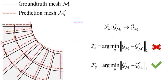
Figure 1. Schematic of mesh mismatch and invalid optimization mode.

This critical oversight propagates physical field prediction errors to geometrically mismatched mesh points, where nodal position deviations corrupt gradient computations and compound solution inaccuracies.

To overcome this limitations, we propose a novel point-wise full-field physics neural mapping framework for large deformation. The core of our approach formulates the physical field prediction as a two-stage computational process. First, a graph neural network constructs the mapping from initial to deformed boundary configurations under prescribed mechanical constraints, establishing the deformed geometry. Subsequently, a residual network architecture establishes direct coordinate-to-physics mappings within the deformed domain. This point-wise learning strategy inherently eliminates errors induced by mesh misalignment. Furthermore, we introduce a displacement-fused encoding layer that enhances field prediction accuracy by integrating nodal displacement information via a guiding branch. The proposed method is rigorously validated on a comprehensive metal forming dataset covering diverse deformation scenarios, demonstrating superior performance against existing deep learning baselines. The main contributions of this work are summarized as follows:

• A end-to-end deep learning framework for accurate full-field physics prediction is proposed for large deformation problems.
• A novel two-stage neural architecture that structures the large deformation computation problem into geometric prediction and physical resolution phases, inherently circumventing mesh-mismatch errors by establishing direct mappings from spatial coordinates to physical field values.
• A displacement-aware encoding mechanism that incorporates nodal displacement constraints through a guided learning branch is introduced, which significantly enhancing prediction accuracy.
• Experimental results on an industrial-scale metal forming dataset show our method achieves 36–98% reduction in mean absolute error compared to existing deep learning baselines.

2. Methodology

In this section, we first introduce the numerical formulation of large thermoplastic deformation in Section 2.1. We then introduce the problem formulation of parameterized learning methods in Section 2.2. In Section 2.3, we introduce the proposed point-wise full-field physics neural mapping framework.

2.1. Numerical Formulation of Large Thermoplastic Deformations

The governing equation is derived from the linear momentum balance in the reference configuration [24]

$$\nabla ·(\mathbf{F}·\mathbf{S})+{\mathbf{b}}_0=\mathbf{0},$$

(2)

where ∇ is the divergence operator in the reference configuration, $\mathbf{F}=\partial \mathbf{x}/\partial \mathbf{X}$ is the deformation gradient, $\mathbf{S}$ is the second Piola–Kirchhoff stress tensor, and ${\mathbf{b}}_0$ is the body force per unit reference volume. The weak form is obtained by multiplying by a test function $\delta \mathbf{u}$ and integrating over the reference domain $\Omega$

$${\int }_{\Omega }\delta \mathbf{E}:\mathbf{S}d\Omega ={\int }_{\Omega }\delta \mathbf{u}·\mathbf{b}d\Omega +{\int }_{\partial \Omega }\delta \mathbf{u}·\mathbf{t}d\Gamma ,$$

(3)

where $\delta \mathbf{E}={\displaystyle \frac{1}{2}}({\mathbf{F}}^T·\delta \mathbf{F}+\delta {\mathbf{F}}^T·\mathbf{F})$ is the variation of the Green–Lagrange strain tensor with $\delta \mathbf{F}={\displaystyle \frac{\partial \delta \mathbf{u}}{\partial \mathbf{X}}}$, and $\mathbf{t}$ is the surface traction per unit reference area. The nonlinear finite element discretization of Equation (3) leads to the following incremental equilibrium equation:

$$\mathbf{R}\left(\mathbf{u}\right)={\mathbf{F}}^{\mathrm{int}}\left(\mathbf{u}\right)-{\mathbf{F}}^{\mathrm{ext}}=\mathbf{0},$$

(4)

where $\mathbf{R}$ is the residual force vector, ${\mathbf{F}}^{\mathrm{int}}$ is the internal force vector, and ${\mathbf{F}}^{\mathrm{ext}}$ is the external force vector. The internal force vector is computed as

$${\mathbf{F}}^{\mathrm{int}}={\int }_{\Omega }{\mathbf{B}}^T·\mathbf{P}d\Omega ,$$

(5)

where $\mathbf{P}=\mathbf{F}·\mathbf{S}$ is the first Piola–Kirchhoff stress tensor, $\mathbf{B}$, is the strain–displacement matrix where the axisymmetric components can be expressed as

$$\mathbf{B}=\left[\begin{array}{cc}{\displaystyle \frac{\partial N_i}{\partial r}}& 0\\ 0& {\displaystyle \frac{\partial N_i}{\partial z}}\\ {\displaystyle \frac{N_i}{r}}& 0\\ {\displaystyle \frac{\partial N_i}{\partial z}}& {\displaystyle \frac{\partial N_i}{\partial r}}\end{array}\right],i=1,2,\dots ,L,$$

(6)

where $N_i=N_i(r,z)$ denotes the shape function of i-th node, and L denotes the number of nodes.

The temperature evolution is governed by the heat conduction equation [25]

$$k{\nabla }^{2}T+\dot{q}=\rho c{\displaystyle \frac{\partial T}{\partial t}},$$

(7)

where T denotes temperature, $\rho$ (kg·m⁻³) denotes the density, c (J·kg⁻¹·°C⁻¹) denotes the specific heat, k (W·m⁻¹·°C⁻¹) denotes the thermal conductivity, and $\dot{q}$ (W·m⁻³) denotes the heat source term representing the thermal energy generated by plastic deformation work. $\dot{q}$ is determined by [26]

$$\dot{q}=\eta \overline{\sigma }\dot{\overline{\epsilon },}$$

(8)

where $\overline{\sigma }$ (MPa) denotes the effective flow stress, $\dot{\overline{\epsilon }}$ (s⁻¹) denotes the effective strain rate, and $\eta$ denotes the efficiency of conversion of deformation energy to heat. Generally, the value of $\eta$ is 0.9 [27]. The corresponding weak form is

$${\int }_{\Omega }\delta T\rho c_p{\displaystyle \frac{\partial T}{\partial t}}d\Omega +{\int }_{\Omega }\nabla \delta T·k\nabla Td\Omega ={\int }_{\Omega }\delta T\dot{q}d\Omega +{\int }_{{\Gamma }_q}\delta T{q}_{n}d\Gamma ,$$

(9)

where $q_n$ denotes the boundary heat flux, and ${\Gamma }_q$ denotes the heat flux boundary.

The finite element discretization yields the system

$${\mathbf{C}}^t\dot{\mathbf{T}}+{\mathbf{K}}^t\mathbf{T}=\mathbf{Q},$$

(10)

with the matrices defined as

$$\begin{array}{cc}\hfill {\mathbf{C}}^t& ={\int }_{\Omega }{\mathbf{N}}^T\rho c_p\mathbf{N}d\Omega ,\hfill \end{array}$$

(11)

$$\begin{array}{cc}\hfill {\mathbf{K}}^t& ={\int }_{\Omega }\nabla {\mathbf{N}}^{T}k\nabla \mathbf{N}d\Omega ,\hfill \end{array}$$

(12)

$$\begin{array}{cc}\hfill \mathbf{Q}& ={\int }_{\Omega }{\mathbf{N}}^T\dot{q}d\Omega +{\int }_{{\Gamma }_q}{\mathbf{N}}^T{q}_{n}d\Gamma ,\hfill \end{array}$$

(13)

where $\mathbf{N}=[N_1,N_2,\dots ,N_L]$ contains the element shape functions and $\nabla \mathbf{N}={[{\displaystyle \frac{\partial N_i}{\partial r}},{\displaystyle \frac{\partial N_i}{\partial z}}]}^T$ for 2D axisymmetric problems.

2.2. Problem Formulation

Although FEM provides accurate solutions to the equations in Section 2.1 through iterative numerical schemes, it is hampered by high computational cost and lacks a flexible input–output mechanism. The rapid advancement of data-driven approaches, particularly deep learning techniques, has enabled the successful implementation of neural networks that directly model the mapping from boundary conditions to physical fields using finite element data. Let ${\mathcal{G}}_0=({\mathbf{x}}_0,{\mathbf{u}}_0,{\mathbf{u}}_b)$ denote the initial state, where ${\mathbf{x}}_0,{\mathbf{u}}_0,{\mathbf{u}}_b$ denote the initial coordinates, the initial states, and the boundary condition of the observation points. Let ${\mathcal{G}}_t=({\mathbf{x}}_t,{\mathbf{u}}_t)$ denote the state after deformation, where ${\mathbf{x}}_t,{\mathbf{u}}_t$ denote the coordinates and the corresponding physical quantities after deformation. The model aims to learn a $\theta$-parameterized mapping

$${\mathcal{F}}_{\theta }:{\mathcal{G}}_0\mapsto {\mathcal{G}}_t,$$

(14)

by

$${\mathcal{F}}_{\theta }^{*}=arg\underset{\theta }{min}\mathcal{L}({\mathcal{F}}_{\theta },{\mathcal{G}}_t),$$

(15)

where $\mathcal{L}$ denotes the loss function formulated by

$$\mathcal{L}={\mathbb{E}}_{({\mathcal{G}}_{0,i},{\mathcal{G}}_{t,i})\in \mathcal{D}}\left|\right|{\mathcal{F}}_{\theta }\left({\mathcal{G}}_{0,i}\right)-{\mathcal{G}}_{t,i}{\left|\right|}_2,$$

(16)

where $\mathcal{D}$ denotes the dataset, ${\mathcal{G}}_{0,i},{\mathcal{G}}_{t,i}$ denotes the initial state vector and the state vector after deformation of the i-th sample, respectively. The validity of Equation (16) is contingent upon strict equivalence between predicted and ground truth coordinates, i.e., ${\mathbf{x}}_t^{*}={\mathbf{x}}_t$, where ${\mathbf{x}}_t^{*}$ denotes the predicted coordinates. However, existing methods overlook this critical constraint, leading to erroneous propagation of prediction errors during model training and fundamentally limiting accuracy.

To circumvent prediction errors induced by spatial coordinate mismatches, we propose a novel paradigm that directly models the mapping between coordinates and physical quantities within the deformed fields. Let ${\mathbf{x}}_q\in {\Omega }_t$ denote the coordinates of the query points within the deformed domain ${\Omega }_t$. The mapping is formulated by

$${\mathcal{F}}_{\theta :\mathbf{u}}:({\mathbf{x}}_q,{\mathbf{u}}_0,{\mathbf{u}}_b)\mapsto {\mathbf{u}}_q,$$

(17)

where ${\mathbf{u}}_q$ denotes the corresponding physical quantities of ${\mathbf{x}}_q$. The learning problem is formulated as

$${\mathcal{F}}_{\theta :\mathbf{u}}^{*}=argmin{\mathbb{E}}_{[{\mathbf{x}}_q\in {\mathbf{x}}_t,{\mathbf{u}}_q\in {\mathbf{u}}_t,({\mathbf{x}}_t,{\mathbf{u}}_0,{\mathbf{u}}_b,{\mathbf{u}}_t)\sim \mathcal{D}]}\left|\right|{\mathcal{F}}_{\theta :\mathbf{u}}({\mathbf{x}}_q,{\mathbf{u}}_0,{\mathbf{u}}_b)-{\mathbf{u}}_q{\left|\right|}_2.$$

(18)

Note that during the training stage, ${\mathbf{x}}_t\in {\Omega }_t$ serves as predefined point coordinates for supervised learning. However, during inference, the model must first predict ${\Omega }_t$. ${\Omega }_t$ is determined by $\partial {\Omega }_t$, which is defined by the boundary points. Let ${\mathbf{x}}_0^B\in {\Omega }_0,{\mathbf{x}}_t^B\in {\Omega }_t$ denote the boundary points coordinates before and after deformation. we can learn a mapping

$${\mathcal{F}}_{\theta :B}:({\mathbf{x}}_0^B,{\mathbf{u}}_0,{\mathbf{u}}_b)\mapsto {\mathbf{x}}_t^B$$

(19)

to determine ${\Omega }_t$. The learning problem of ${\mathcal{F}}_{\theta :B}$ can be formulated as

$${\mathcal{F}}_{\theta :B}^{*}=argmin{\mathbb{E}}_{({\mathbf{x}}_0^B,{\mathbf{x}}_t^B,{\mathbf{u}}_0,{\mathbf{u}}_b)\sim \mathcal{D}}\left|\right|{\mathcal{F}}_{\theta :B}({\mathbf{x}}_0^B,{\mathbf{u}}_0,{\mathbf{u}}_b)-{\mathbf{x}}_t^B{\left|\right|}_2.$$

(20)

2.3. The Proposed Method

The proposed framework is shown in Figure 2. The architecture integrates two functionally specialized modules: boundary geometric prediction module and physical field prediction module. Firstly, the boundary geometric prediction module processes boundary coordinates, initial conditions, and boundary constraints to predict the deformed boundary point set ${\Omega }_t$. Then, this predicted geometry undergoes discretization to produce sampling points ${\mathbf{x}}_q$. Last, the coordinates together with the initial state ${\mathbf{u}}_0$ and boundary condition ${\mathbf{u}}_b$ are fed into the physical field prediction module to compute the corresponding field distribution ${\mathbf{u}}_q$. The details are as follows.

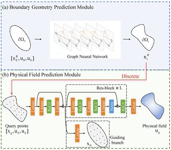
Figure 2. The proposed framework. (a) The schematic of the boundary geometry prediction module. (b) The framework of the physical field prediction module.

Boundary geometry prediction module. The boundary geometry module is designed to predict the deformed boundary node coordinates from the initial configuration under given boundary conditions. The module is implemented as a GNN operating on a graph representation of the boundary nodes. The design consists of the following key components. The graph is constructed with boundary nodes as vertices. The i-th node is associated with its initial coordinates ${\mathbf{x}}_{0,i}^B\in {\mathbb{R}}^{D_C}$ (where $D_C=2$ for 2D problems), initial state ${\mathbf{u}}_{0,i}\in {\mathbb{R}}^{D_I}$ (e.g., initial displacement or velocity), and boundary condition ${\mathbf{u}}_{b,i}\in {\mathbb{R}}^{D_B}$ (e.g., prescribed displacement or traction).

The graph’s adjacency structure is constructed using Delaunay triangulation applied to the initial boundary nodal coordinates. This computational geometry approach generates a mesh of non-overlapping triangles while naturally establishing connections between nodes based on spatial proximity. For each node i, the set of neighbors $\mathcal{N}\left(i\right)$ is determined by natural geometric adjacency relationships established through this triangulation. The graph remains undirected, with edges formed exclusively between nodes connected by triangulation edges.

Boundary conditions are encoded directly into the node features. For Dirichlet conditions (prescribed displacements), ${\mathbf{u}}_{b,i}$ represents the prescribed displacement vector. For Neumann conditions (tractions), it represents the traction vector. The encoding functions ${\mathcal{E}}^v$ and ${\mathcal{E}}^e$ are implemented as linear layers that project the input features to a hidden dimension $D_H$. Specifically, the node embedding ${\mathit{v}}_i$ and edge embedding ${\mathit{e}}_{ij}$ are calculated by

$$\begin{array}{cc}\hfill {\mathit{v}}_i& ={\mathcal{E}}^v({\mathbf{x}}_{0,i}^B,{\mathbf{u}}_{0,i},{\mathbf{u}}_{b,i})\in {\mathbb{R}}^{D_H},\hfill \\ \hfill {\mathit{e}}_{i,j}& ={\mathcal{E}}^e(d_{ij},{\mathbf{d}}_{ij})\in {\mathbb{R}}^{D_H},\hfill \end{array}$$

(21)

where $d_{i,j}=\left|\right|{\mathbf{x}}_{0,i}^B-{\mathbf{x}}_{0,j}^B{\left|\right|}_2$ denotes the Euclidean distance, and ${\mathbf{d}}_{i,j}=({\mathbf{x}}_{0,i}^B-{\mathbf{x}}_{0,j}^B)/d_{i,j}$ denotes the unit direction vector.

The GNN performs $T_p$ steps of message passing (by default, $T_p=5$). At each step $\tau$, the message from node j to i is computed as follows:

$$\begin{array}{cc}\hfill {\mathit{m}}_{ij}^{\tau }& =(1-\gamma ){\mathit{v}}^{\tau }+\gamma {\mathit{e}}_{ij}^{\tau },\hfill \\ \hfill \gamma & =\sigma \left(\mathrm{MLP}\left({\mathit{e}}_{ij}^{\tau }\right)\right),\hfill \end{array}$$

(22)

where $\sigma$ here denotes the Sigmoid function, ensuring $\gamma \in (0,1)$. This allows the network to dynamically balance node and edge information. The node feature is updated by aggregating messages from all neighbors:

$${\mathit{v}}_i^{\tau +1}={\displaystyle \frac{1}{\left|\mathcal{N}\right(i\left)\right|}}\sum _{j\in \mathcal{N}\left(i\right)}{\mathit{m}}_{ij}^{\tau }+W·{\mathit{v}}_i^{\tau },$$

(23)

where W is a linear transformation. This update rule combines neighborhood information with the node’s own state, preserving historical information. After $T_p$ message passing steps, the final node features ${\mathit{v}}_i^{T_p}$ are passed through a linear layer to predict the deformed coordinates ${\mathbf{x}}_{t,i}$

$${\mathbf{x}}_{t,i}=\mathrm{Linear}\left({\mathit{v}}_i^{T_p}\right).$$

(24)

This module is trained end-to-end using mean squared error (MSE) loss between predicted and ground truth coordinates of the boundary nodes.

Discretization. This module performs domain discretization during the inference phase, implemented using the open-source library PyGmsh [28]. By inputting boundary point sets, it discretizes the solution domain into a specified number of discrete points.

Physical field prediction module. The physical field prediction module consists primarily of an encoding layer, a ResNet-based feature transformation layer, and a prediction layer. The encoding layer first projects input features to a target dimension $D_H$ via a linear layer, followed by an MLP with one hidden layer to perform feature encoding. The encoder layer follows

$$\begin{array}{cc}\hfill {\mathcal{X}}_i^p& =\mathrm{Linear}({\mathbf{x}}_{q,i},{\mathbf{u}}_b)\in {\mathbb{R}}^{D_H};\hfill \\ \hfill {\mathcal{X}}_i^e& ={\mathcal{X}}_i^p+\mathrm{MLP}\left({\mathcal{X}}_i^p\right).\hfill \end{array}$$

(25)

${\mathcal{X}}_i^e\in {\mathbb{R}}^{D_H}$ is then transformed by the resnet layer with L residual blocks. The l-th block follows

$$\begin{array}{cc}\hfill {\mathcal{X}}_i^{r,l+1}& =\mathrm{ReLU}\left({\mathcal{X}}_i^{r,l}+\mathrm{BatchNorm}\left(\mathrm{MLP}\left({\mathcal{X}}_i^{r,l}\right)\right)\right),\hfill \end{array}$$

(26)

where ${\mathcal{X}}_i^{r,l}\in {\mathbb{R}}^{D_F}$ denotes the input of the residual block and ${\mathcal{X}}_i^e$ is the input of the first layer.

Finally, the prediction of i-th query node ${\mathbf{u}}_i^{*}\in {\mathbb{R}}^{D_F}$ is calculated by

$${\mathbf{u}}_i^{*}=\mathrm{Linear}\left({\mathcal{X}}_i^{r,L}\right)\in {\mathbb{R}}^{D_F},$$

(27)

where $D_F$ denotes the dimension of ${\mathbf{u}}_i^{*}$. During training, we use ${\mathbf{x}}_t$ as the query coordinates ${\mathbf{x}}_q$ to learn the functional mapping between coordinates and the corresponding physical quantities. The guiding branch incorporates displacement prediction loss into the network, enabling the fusion of displacement information. The loss function is formulated by

$${\mathcal{L}}_F={\mathcal{L}}_f+\alpha {\mathcal{L}}_g,$$

(28)

where ${\mathcal{L}}_f$ is the MSE of ${\mathbf{u}}_t$, ${\mathcal{L}}_g$ is the MSE of the guiding branch that predicts ${\mathbf{u}}_0$, and $\alpha$ denotes the scale factor. We further study the effectiveness of the guiding branch in Section 4.3.

3. Experiment Setting

This section details the experimental setup. Section 3.1 describes the dataset used for method validation. Section 3.2 specifies the default settings of our proposed model, while Section 3.3 outlines the baseline models implemented for comparison. Finally, Section 3.4 presents the evaluation metrics employed to assess model performance.

3.1. Dataset

Metal thermoplastic forming represents a typical large deformation process. The workpiece undergoes geometric deformation due to the compression of the dies, with the internal physical fields distribution variations. Figure 3a illustrates a typical example of cylindrical compression molding, along with the distribution of x-direction strain component after the forming process.

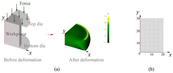
Figure 3. (a) The schematic diagram of Metal thermoplastic forming and the field distribution (x-direction strain) after forming (1/4 part of the 3D model) (b) Geometrical setup of the cross-section of the workpiece for FEM simulations. The cross-section is discretized into 1080 nodes (27 along x-direction and 40 along y-direction). The height and radius of the workpiece are 30 mm and 20 mm, respectively.

To obtain the physical field variations during the forming process, numerical simulations are performed using the DEFORM-3D software (version V11.0). Taking advantage of geometric symmetry, a 2D axisymmetric module is employed to efficiently simulate the deformation process. The geometry of the axially symmetric section of the workpiece is detailed in Figure 3b. The height and radius of the workpiece are set as 30 mm and 20 mm, respectively. The cross section is discretized into a structured grid of 1080 nodes (27 along the x-direction and 40 along the y-direction). The material behavior is modeled using the built-in constitutive model for 2014 aluminum alloy (2014Al). The initial temperature of the workpiece is $T_0$. The dies are set as rigid body with an initial temperature $T_d$. During the forming process, the bottom die remains stationary while the top die moves downward with a constant speed v. The maximum stroke is set as 15 mm. The type of contact friction between the mold and the workpiece is set as Coulomb friction, with a friction coefficient $\mu \in \{0.12,0.2\}$. The number of time steps of the simulation is 30, i.e., the stroke of the top die between the adjacent two time steps is 0.5 mm.

We establish a dataset that records the simulation results, including nodal displacement, temperature, stress with its components, and strain with its components, of all the 30 time steps. The details of the process parameters, including $\mu ,T_0,T_d,v$, are listed in Table 1. The total number of process parameters combinations is 7480, corresponding to the number of samples of the dataset. The details of the physical quantities in the dataset are shown in Table 2.

Table 1. Details of the process parameters.

Symbol	Min	Max	Step	Count	Unit	Description
$\mu$	0.12	0.2	-	2	-	Friction factor
$T_0$	400	480	5	17	°C	Initial temperature of the workpiece
$T_d$	200	300	10	11	°C	Initial temperature of the dies
v	1	20	1	20	mm/s	Compress velocity of the top die

Table 2. Details of the physical quantities.

Features	Min	Max	Unit	Description
$\mathcal{T}$	201	480	°C	Temperature
${\epsilon }_{xx}$	0	0.85	-	x-direction normal strain
${\epsilon }_{yy}$	−1.12	0	-	y-direction normal strain
${\epsilon }_{\theta }$	0	0.45	-	Hoop strain
${\epsilon }_{xy}$	−1.47	1.48	-	Shear strain
${\sigma }_{xx}$	−150	74	MPa	x-direction normal stress
${\sigma }_{yy}$	−357	51	MPa	y-direction normal stress
${\sigma }_{\theta }$	−210	153	MPa	Hoop stress
${\sigma }_{xy}$	−69	80	MPa	Shear stress

3.2. Implementation

The dataset is split into training, validation, and test sets with a ratio of 7:1:2. The partitioning is designed to evaluate the model’s performance under extrapolation conditions, particularly for high-temperature regimes where material behavior exhibits strong nonlinearities. Specifically, the training set (70% of samples) encompasses the low-to-medium temperature range ($T_0$ = 400–455 °C), where conventional plastic deformation mechanisms dominate. The validation set (10%) contains transitional temperature conditions ($T_0$ = 460–465 °C) to monitor training progress and prevent overfitting. Most critically, the test set (20%) is exclusively composed of high-temperature scenarios ($T_0$ = 470–480 °C) that approach the recrystallization threshold of 2014 aluminum alloy.

For the proposed model, we take $\left[T_0\right]$ as the nodal initial state ${\mathbf{u}}_{0,i}$, $[\mu ,T_d,v,s]$ as the nodal boundary condition ${\mathbf{u}}_{d,i}$, where s denotes the displacement of the top die. By default, the hidden dimension $D_H$ is 128. The total number of message passing steps is 5. The number of residual blocks L is 3.

3.3. Baselines

We take CrystalMind [22] and DeepForge [23] as the baseline models. These models are typically optimized using the objective function defined in Equation (16). The network architectures of these models are detailed in Table A1, Table A2 and Table A3.

3.4. Metrics

We evaluate the geometrical deformation prediction performance and the physical fields reconstruction performance by mean absolute error (MAE). To evaluate the physical fields reconstruction performance, we apply the Inverse Distance Weighting (IDW) algorithm [29], which estimates unknown values at specific locations based on nearby points, to calculate the predictions on the test set nodal coordinates for CrystalMind and DeepForge. Given $N_I$ neighbors ${\mathcal{N}}_I={\{x_i,y_i,{\psi }_i\}}_{i=1}^{N_I}$, the interpolated value $\widehat{\psi }$ at $(x,y)$ is:

$$\widehat{\psi }(x,y)=\left\{\begin{array}{cc}{\displaystyle \frac{{\sum }_{i=1}^{N_I}{w}_i(x,y){\psi }_i}{{\sum }_{i=1}^{N_I}{w}_i(x,y)}},\hfill & \mathrm{if}{d}_i(x,y)\ne 0,\hfill \\ {\psi }_i,\hfill & \mathrm{if}{d}_i(x,y)=0,\hfill \end{array}\right.$$

(29)

where $w_i(x,y)$ is calculated by

$$\begin{array}{cc}\hfill w_i(x,y)& =\left\{\begin{array}{cc}{\displaystyle \frac{1}{d_i(x,y)}},\hfill & \mathrm{if}(x_i,y_i)\in \mathcal{N},\hfill \\ 0,\hfill & \mathrm{otherwise},\hfill \end{array}\right.\hfill \\ \hfill d_i(x,y)& =\sqrt{{(x-x_i)}^2+{(y-y_i)}^2}.\hfill \end{array}$$

(30)

By default, $N_I=4$.

4. Results

This section evaluates the performance of the proposed method through comprehensive experiments. Section 4.1 assesses the boundary geometry prediction accuracy in comparison with baseline models. Section 4.2 extends the comparison to full-field reconstruction performance across all physical quantities. Further analysis includes a study on model parameter scaling in Section 4.3 and model computation efficiency in Section 4.4. An investigation of the guiding branch’s influence on prediction accuracy in Section 4.5.

4.1. Boundary Geometry Prediction Result

The performance of the model is evaluated by the Euclidean distance between the predicted points and the ground truth boundary (denoted as $\mathsf{\Delta }d$). Figure 4 shows the error map of the boundary nodes’ coordinates prediction results of the proposed model on a test sample. The statistical result on the test set is shown in Figure 5. The mean values of $\mathsf{\Delta }d$ on the test set of our proposed model, CrystalMind, and DeepForge are 0.12 mm, 0.16 mm, and 0.19 mm. Notably, as illustrated in the figure, our model outperforms the alternatives in stability, exhibiting the smallest $\mathsf{\Delta }d$ fluctuations (standard deviation), with CrystalMind ranking second. DeepForge, on the other hand, shows both the highest average $\mathsf{\Delta }d$ and the most significant variation. This stability arises from our dedicated boundary geometry module, which avoids mesh-misalignment errors by focusing solely on coordinate prediction, whereas CrystalMind and DeepForge suffer from error propagation due to their end-to-end learning of coupled geometry-physics mappings. DeepForge’s AutoEncoder architecture, which lacks explicit geometric inputs, further amplifies instability when reconstructing high-dimensional outputs.

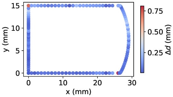
Figure 4. Error map of the boundary nodes position prediction result of the proposed model.

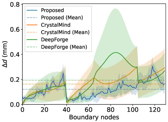
Figure 5. Statistic results of $\mathsf{\Delta }d$ on the test set. The solid line represents the mean value of each point, the shaded area represents the standard deviation, and the dotted line represents the mean value of all the points.

4.2. Full-Field Physics Reconstruction Result

Figure 6 visualizes the full-field physics reconstruction result of our proposed model on a test sample. The result encompasses reconstruction for nine physical quantities, including temperature, strain components, and stress components, as well as their discrepancies compared to the ground truth distributions. For brevity, we present only the final time step’s prediction results. As demonstrated in the result, our approach can reliably reconstruct the field distributions for all relevant physical quantities.

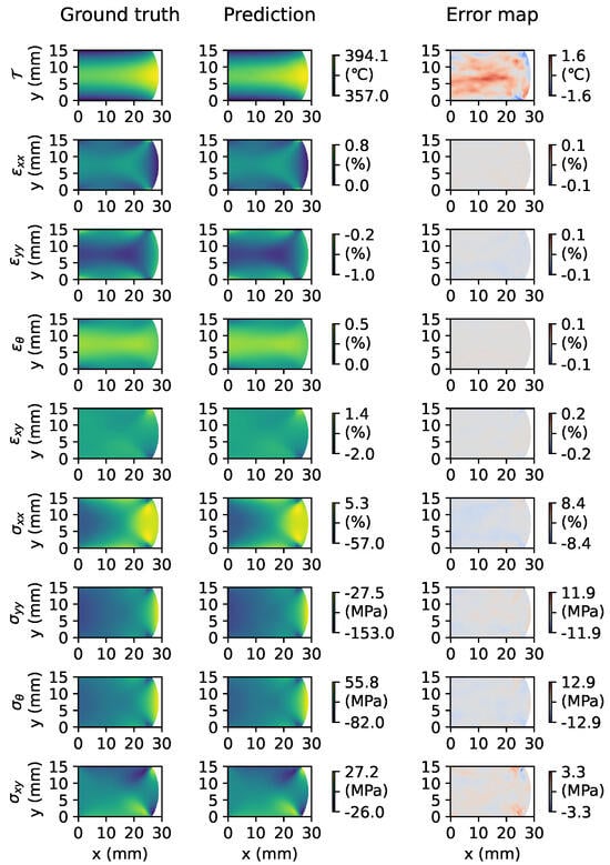
Figure 6. Visualization of the full-field physics reconstruction result of the proposed model.

The MAEs of all the nine physical quantities on the test set are illustrated in Figure 7. Our proposed model demonstrates overall lower MAE compared to the other two models, with only slightly higher values for ${\epsilon }_{xy}$ (0.01 vs. 0.007) and ${\sigma }_{xy}$ (0.654 vs. 0.503) when compared to CrystalMind. DeepForge demonstrates significantly inferior performance compared to our model, exhibiting MAEs that are consistently 10 times higher across all evaluated physical quantities. This model exemplifies the intrinsic limitations of sequence-tracking-based methods, where the non-negligible nodal position prediction errors can significantly amplify inaccuracies in physical field predictions.

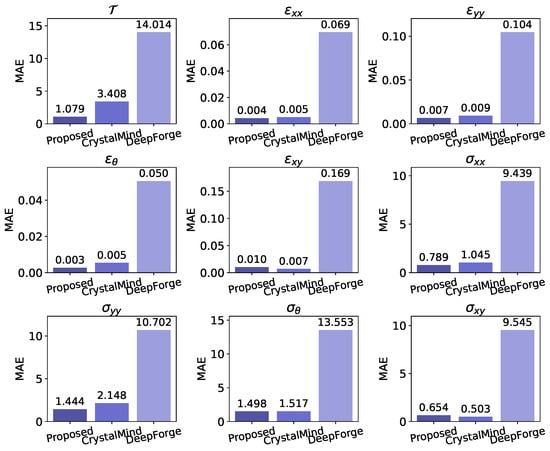
Figure 7. MAEs of the physical field prediction results.

In contrast, our proposed model fundamentally transforms the prediction paradigm by directly establishing the mapping between arbitrary point’s coordinates within deformed domains and their corresponding physical quantities. This architecture intrinsically ensures correspondence between ‘keys’ (coordinates) and ‘values’ (physical quantities), thereby achieving significant error reduction.

4.3. Analysis of Model Size Impact on Performance

We investigate the impact of model size on performance, with quantitative results presented in Figure 8. We scaled the hidden dimension $D_H$ across three settings (32, 128, and 512). This resulted in the boundary prediction module with 0.004 M, 0.052 M, and 0.8 M parameters, and the field distribution prediction module with 0.011 M, 0.168 M, and 2.636 M parameters, respectively. The results demonstrate a clear trend of decreasing MAE with increasing model parameters. Specifically, for the boundary prediction module, when the parameter count increased from 0.004 M to 0.8 M, the deviation in d decreased significantly from 0.21 to 0.05, representing a 75% reduction. Remarkably, compared to CrystalMind (28.98 M parameters with MAE 0.163), our model achieves approximately 60% higher accuracy while using only 3% of its parameter count (Note that the total number of parameters of CrystalMind is referenced because the nodal coordinates prediction and physical fields prediction are intrinsically coupled).

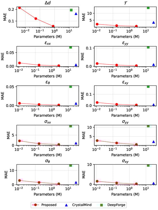
Figure 8. Model performance vs. number of parameters.

On the other hand, scaling the physical field prediction module from 0.011 M to 2.636 M parameters yielded substantial accuracy gains, with improvement rates ranging from 68% to 85% across different physical quantities. Comparative analysis shows that our method achieves 36.2–79.8% higher accuracy in physical fields prediction with 89.7% parameter reduction compared to CrystalMind (2.636 M vs. 28.98 M parameters). Furthermore, our method achieves a 94–98% reduction in physical field prediction error compared to DeepForge (13.76 M parameters).

The proposed model establishes relationships between arbitrary point locations within the deformed field and their corresponding physical quantities, rather than modeling the mappings between initial states and the states after deformation. This fundamental innovation effectively circumvents prediction errors caused by mesh mismatches, not only significantly enhancing prediction accuracy but also dramatically reducing parameter requirements compared to existing methods.

4.4. Computation Efficiency

To quantify the computational efficiency, we evaluate the wall-clock training time as well as the model size, inference memory usage, and inference speed of the three models. The inference task requires simultaneous reconstruction of the geometrical deformation as well as the full-field distributions including the temperature field, strain field, and stress field for 30 time steps throughout the entire forming process. Both the proposed model and CrystalMind enforce independence inference among different time steps, implementing a parallel computation paradigm that enables full-progress physical field reconstruction through batch mode. In contrast, DeepForge requires sequential execution during full-progress inference, as each time step depends on the external observed surface temperature as input (note that it is regarded as a known item during the training process).

We executed 500 independent inference runs for each model on both CPU (Intel Xeon Silver 4314; Intel Corporation, Santa Clara, CA, USA) and GPU (NVIDIA RTX 3090 24 GB; NVIDIA Corporation, Santa Clara, CA, USA) platforms, recording precise inference latencies using high-resolution timers (ns precision). The complete comparisons are presented in Table 3. The results indicate a distinct trade-off between inference speed and resource consumption across the different approaches. In terms of inference speed on a CPU, DeepForge demonstrates the shortest computation time (71.88 ± 1.85 ms), followed by CrystalMind (115.22 ± 7.65 ms), while our proposed method requires the longest processing time (167.53 ± 3.90 ms). However, a markedly different trend is observed for GPU acceleration. CrystalMind achieves a significantly faster inference speed (4.47 ± 0.74 ms) than both our method (95.86 ± 0.63 ms) and DeepForge (20.79 ± 3.05 ms) on the GPU. Regarding memory footprint, our method consumes a moderate amount of memory (1.56 GB), which is comparable to DeepForge (1.48 GB) and substantially lower than CrystalMind (2.70 GB).

Table 3. Inference time and memory usage of the models.

	The Proposed Method	CrystalMind	DeepForge
CPU time (ms)	167.53 ± 3.90	115.22 ± 7.65	71.88 ± 1.85
GPU time (ms)	95.86 ± 0.63	4.47 ± 0.74	20.79 ± 3.05
Memory usage (GB)	1.56	2.70	1.48

The observed differences in computational efficiency can be attributed to the underlying architectural designs of the models. The superior GPU performance of CrystalMind likely stems from a highly optimized computational graph and a higher degree of parallelism inherent in its single-stage, end-to-end architecture. In contrast, the two-stage prediction pipeline of our method, which involves sequential processing by distinct geometric and physical field modules, introduces inherent computational overhead, resulting in longer CPU and GPU times. However, this architectural choice also allows for more compact intermediate representations, contributing to our method’s moderate memory usage. The low memory footprint of DeepForge is consistent with its autoencoder-based structure, which typically operates on a compressed latent representation. Ultimately, the higher computational cost of our method is the direct trade-off for its enhanced prediction accuracy, as demonstrated in the previous sections, making it particularly suitable for applications where precision is paramount over real-time speed.

4.5. Influence of the Guiding Branch

In this section, we analyze the influence of the guiding branch. We first study the performance with different $\alpha$. By default, $D_H=128$. The results are demonstrated in Table 4. We find that as $\alpha$ decreases from 10 to 0.1, ${\mathcal{L}}_f$ shows a slight improving trend (decreasing from approximately 0.00312 to 0.00285), with the minimum value achieved at $\alpha =0.2$. Conversely, ${\mathcal{L}}_g$ exhibits a consistent and significant deterioration (increasing from 0.00506 to 0.00647) as $\alpha$ decreases. This relationship is expected, as a lower $\alpha$ reduces the penalty associated with ${\mathcal{L}}_g$ during training, allowing the model to prioritize the minimization of ${\mathcal{L}}_f$ at the expense of ${\mathcal{L}}_g$. While $\alpha =1$, the model represents a balanced compromise between ${\mathcal{L}}_f$ and ${\mathcal{L}}_g$.

Table 4. ${\mathcal{L}}_f$ and ${\mathcal{L}}_g$ of the last training epoch with different $\alpha$.

	$\mathit{\alpha }$ = 10	$\mathit{\alpha }$ = 5	$\mathit{\alpha }$ = 2	$\mathit{\alpha }$ = 1	$\mathit{\alpha }$ = 0.5	$\mathit{\alpha }$ = 0.2	$\mathit{\alpha }$ = 0.1
${\mathcal{L}}_f$	0.003121	0.003332	0.003013	0.002804	0.002833	0.002628	0.002847
${\mathcal{L}}_g$	0.005064	0.005033	0.004990	0.005083	0.005883	0.006138	0.006469

Figure 9 compares the training loss with (w/) and without (w/o) the guiding branch, where $\alpha$ is set as 1 and 0, respectively. ${\mathcal{L}}_f$ and ${\mathcal{L}}_g$ are 0.0030 and 0.43 of the last training epoch for the model without guiding branch. Experimental results confirm that activating the guiding branch significantly reduces the physical field prediction error ${\mathcal{L}}_f$, demonstrating its effectiveness in enhancing prediction accuracy through the integration of displacement-related information. Furthermore, even when the guiding branch is disabled, a consistent decrease of ${\mathcal{L}}_g$ is observed throughout training, of which dropping from approximately 0.6 initially to 0.43 upon convergence. This trend clearly indicates a mutually reinforcing relationship between displacement and physical field prediction, where improvements in one aspect facilitate learning in the other.

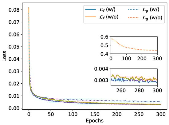
Figure 9. Training loss with/without the guiding branch.

Additionally, we conducted comprehensive tests across different parameter scales, maintaining identical parameterization schemes as established in Section 4.3. By default, $\alpha =1$ for model with guiding branch. As shown in Figure 10, activating the guiding branch consistently improves physical fields prediction accuracy, with more pronounced benefits at larger model sizes. Specifically, for the temperature field at 2.636 M parameters, the prediction error is reduced by 33.8% (from 1.04 to 0.688) when the branch is enabled. The prediction accuracy improvements for other physical fields range from 8% (${\sigma }_{\theta }$) to 38.5% (${\epsilon }_{\theta }$). Experimental results demonstrate that the integration of the guiding branch’s displacement prediction loss yields accuracy improvements for physical fields prediction. This demonstrates the critical role of geometrical deformation awareness in physical field prediction.

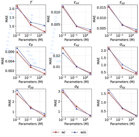
Figure 10. Performance with/without the guiding branch.

5. Discussion

While the proposed method has achieved notable accuracy in physical field prediction for large thermoplastic deformations, we acknowledge several limitations requiring further investigation. Firstly, the current framework does not employ explicit PDE-constrained optimization, it incorporates an implicit physics regularization (nodal displacement) through the guiding branch. This design, inspired by the sequential geometry-physics solution paradigm of numerical methods, provides a flexible inductive bias towards physically consistent solutions. However, incorporating physical constraints into the learning framework represents a particularly meaningful direction for future enhancement for scenarios with well-defined physical relationships. Future work could explore hybrid approaches that combine the proposed learning paradigm with explicit physical constraints for problems where the governing equations are fully known and well-defined. Secondly, while the current validation has been conducted primarily on axisymmetric problems, extending the method to general 3D non-axisymmetric geometries with complex mesh topologies represents a necessary research direction. This expansion would require addressing substantial challenges in spatial representation and computational efficiency. Notably, the proposed method offers a worthy solution to consider. For physical fields prediction tasks involving tens or even hundreds of thousands of mesh nodes with high-dimensional features, it is more effective to establish a functional mapping from nodal coordinates to the corresponding physical quantities, rather than to model the temporal evolution of the large-scale high-dimension nodal sequences. Lastly, while this study demonstrates the framework’s effectiveness on a specific aluminum alloy forming process, the methodology is inherently general. The core innovation lies in the two-stage prediction framework, which bypass mesh-alignment errors, is not specific to a particular material model or process geometry. Future work will rigorously evaluate the transferability of this approach. This will include extending validation to different material classes (e.g., steels, titanium alloys) exhibiting varied hardening and thermal responses, as well as to other forming operations (e.g., rolling, extrusion) with distinct boundary condition complexities. Such studies will further solidify the framework’s potential as a general-purpose tool for high-fidelity deformation modeling.

6. Conclusions

In this paper, we propose a point-wise full-field physics neural mapping framework via boundary geometry constrained for large thermoplastic deformation. We design a two-stage computational framework which first predicts the geometric deformation and then establishes point-wise mappings between coordinates and physical quantities within the deformed domain. By establishing functional mappings between coordinates and their corresponding physical quantities, our approach fundamentally resolves the mesh-mismatch limitations inherent in existing deep learning-based methods. We validate our approach on a metal thermoplastic forming dataset and conduct comparative experiments with other deep learning models. Experiment results demonstrate that the proposed method achieves a 36–98% improvement in MAE compared to other deep learning baselines, confirming its effectiveness for large thermoplastic deformation computation.

References

- Phanden, R.K.; Sharma, P.; Dubey, A. A review on simulation in digital twin for aerospace, manufacturing and robotics. Mater. Today Proc. 2021, 38, 174–178. [Google Scholar] [CrossRef]
- Shan, J.; Zhang, X.; Liu, Y.; Zhang, C.; Zhou, J. Deformation prediction of large-scale civil structures using spatiotemporal clustering and empirical mode decomposition-based long short-term memory network. Autom. Constr. 2024, 158, 105222. [Google Scholar] [CrossRef]
- He, B.; Bai, K.-J. Digital twin-based sustainable intelligent manufacturing: A review. Adv. Manuf. 2021, 9, 1–21. [Google Scholar] [CrossRef]
- Bathe, K.-J.; Ramm, E.; Wilson, E.L. Finite element formulations for large deformation dynamic analysis. Int. J. Numer. Methods Eng. 1975, 9, 353–386. [Google Scholar] [CrossRef]
- Nti, I.K.; Adekoya, A.F.; Weyori, B.A.; Nyarko-Boateng, O. Applications of artificial intelligence in engineering and manufacturing: A systematic review. J. Intell. Manuf. 2021, 33, 1581–1601. [Google Scholar] [CrossRef]
- Wang, B.; Tao, F.; Fang, X.; Liu, C.; Liu, Y.; Freiheit, T. Smart manufacturing and intelligent manufacturing: A comparative review. Engineering 2021, 7, 738–757. [Google Scholar] [CrossRef]
- Pai, P.F.; Palazotto, A.N. Large-deformation analysis of flexible beams. Int. J. Solids Struct. 1996, 33, 1335–1353. [Google Scholar] [CrossRef]
- Bruhns, O.T. Large deformation plasticity: From basic relations to finite deformation. Acta Mech. Sin. 2020, 36, 472–492. [Google Scholar] [CrossRef]
- Jiang, Z.Y.; Tieu, A.K. A simulation of three-dimensional metal rolling processes by rigid–plastic finite element method. J. Mater. Process. Technol. 2001, 112, 144–151. [Google Scholar] [CrossRef]
- Logg, A. Automating the finite element method. Arch. Comput. Methods Eng. 2007, 14, 93–138. [Google Scholar] [CrossRef]
- Shetty, N.; Shahabaz, S.M.; Sharma, S.; Shetty, S. A review on finite element method for machining of composite materials. Compos. Struct. 2017, 176, 790–802. [Google Scholar] [CrossRef]
- Odot, A.; Haferssas, R.; Cotin, S. Deepphysics: A physics aware deep learning framework for real-time simulation. Int. J. Numer. Methods Eng. 2022, 123, 2381–2398. [Google Scholar]
- Deshpande, S.; Lengiewicz, J.; Bordas, S.P.A. Probabilistic deep learning for real-time large deformation simulations. Comput. Methods Appl. Mech. Eng. 2022, 398, 115307. [Google Scholar] [CrossRef]
- Liang, L.; Liu, M.; Martin, C.K.; Sun, W. A deep learning approach to estimate stress distribution: A fast and accurate surrogate of finite-element analysis. J. R. Soc. Interface 2018, 15, 20170844. [Google Scholar] [CrossRef]
- Bolandi, H.; Li, X.; Salem, T.; Boddeti, V.N.; Lajnef, N. Bridging finite element and deep learning: High-resolution stress distribution prediction in structural components. Front. Struct. Civ. Eng. 2022, 16, 1365–1377. [Google Scholar] [CrossRef]
- Zhang, Y.; Li, Q.-J.; Zhu, T.; Li, J. Learning constitutive relations of plasticity using neural networks and full-field data. Extrem. Mech. Lett. 2022, 52, 101645. [Google Scholar]
- Lee, S.; Kim, K.; Kim, N. A preform design approach for uniform strain distribution in forging processes based on convolutional neural network. J. Manuf. Sci. Eng. 2022, 144, 121004. [Google Scholar] [CrossRef]
- Park, J.-H.; Han, B.; Choi, J.; Shin, S.; Kim, N. CNN-based preform design: Effect of training data configuration on strain distribution in forged products. Int. J. Adv. Manuf. Technol. 2024, 135, 4837–4854. [Google Scholar] [CrossRef]
- Kim, K.; Han, B.; Kim, Y.; Kim, N. Detailed preform design procedure considering the effect of heat treatment in IN718 disk forging. J. Mater. Res. Technol. 2024, 30, 4625–4644. [Google Scholar] [CrossRef]
- Cao, J.; Bambach, M.; Merklein, M.; Mozaffar, M.; Xue, T. Artificial intelligence in metal forming. CIRP Ann. 2024, 73, 561–587. [Google Scholar] [CrossRef]
- Lin, Z.; Wang, R.; Hu, Z.; Hu, Z. Surface temperature field real-time reconstruction of hot forging die based on 1DCNN. Int. J. Therm. Sci. 2024, 204, 109206. [Google Scholar] [CrossRef]
- Uribe, D.; Durand, C.; Baudouin, C.; Bigot, R. Accurate real-time modeling for multiple-blow forging. Int. J. Mater. Form. 2024, 17, 57. [Google Scholar] [CrossRef]
- Petrik, J.; Bambach, M. Deepforge: Leveraging AI for microstructural control in metal forming via model predictive control. J. Manuf. Process. 2024, 121, 193–204. [Google Scholar] [CrossRef]
- Castelló, W.B.; Flores, F.G. A triangular finite element with local remeshing for the large strain analysis of axisymmetric solids. Comput. Methods Appl. Mech. Eng. 2008, 198, 332–343. [Google Scholar] [CrossRef]
- Zhang, S.H.; Zhang, G.L.; Liu, J.S.; Li, C.S.; Mei, R.B. A fast rigid-plastic finite element method for online application in strip rolling. Finite Elem. Anal. Des. 2010, 46, 1146–1154. [Google Scholar] [CrossRef]
- Kim, Y.S.; Son, H.S.; Kim, C.I. Rigid–plastic finite element simulation for process design of impeller hub forming. J. Mater. Process. Technol. 2003, 143, 729–734. [Google Scholar] [CrossRef]
- Han, J.; Cheng, Q.; Hu, P.; Xing, H.; Li, S.; Ge, S.; Wang, K. Finite Element Analysis of Large Plastic Deformation Process of Pure Molybdenum Plate during Hot Rolling. Metals 2023, 13, 101. [Google Scholar] [CrossRef]
- A Python Frontend for Gmsh. Available online: https://github.com/nschloe/pygmsh (accessed on 10 February 2022).
- Lu, G.Y.; Wong, D.W. An adaptive inverse-distance weighting spatial interpolation technique. Comput. Geosci. 2008, 34, 1044–1055. [Google Scholar] [CrossRef]
Disclaimer/Publisher’s Note: The statements, opinions and data contained in all publications are solely those of the individual author(s) and contributor(s) and not of MDPI and/or the editor(s). MDPI and/or the editor(s) disclaim responsibility for any injury to people or property resulting from any ideas, methods, instructions or products referred to in the content. |
© 2025 by the authors. Licensee MDPI, Basel, Switzerland. This article is an open access article distributed under the terms and conditions of the Creative Commons Attribution (CC BY) license (https://creativecommons.org/licenses/by/4.0/).