Optimal Parameter Estimation for Solar PV Panel Based on ANN and Adaptive Particle Swarm Optimization

Abstract

Parameter estimation for solar photovoltaic panels is a popular research topic in green energy. Model parameters can be used for fault diagnosis in solar panels. Artificial neural network (ANN) approaches have been developed to estimate the model parameters of solar panels. In this study, an ANN and Adaptive Particle Swarm Optimization (APSO) approach for model parameter estimation of solar panel is proposed. Load perturbation is injected at the output of the solar PV panel, and the load voltage and current time series are measured. The current and voltage vectors are used as inputs for an ANN, which is used as a classifier for the ranges of the model parameters. The population of the APSO is initialized according to the results of the ANN classifier, and the APSO algorithm is then used to estimate the model parameters of the PV panel. Simulations and experimental studies show that the proposed method has better performance than conventional PSO, and it requires a smaller number of generations to achieve an average parameter estimation error of less than 5%.

1. Introduction

Solar photovoltaic panels are popular green energy sources, and ensuring maximum power operation of PV panels is very important in practice [1]. Model parameter estimation [2], health monitoring, and fault diagnosis [3] in PV panels are also popular research topics in green energy. There are many research works published in the area of PV panel model parameter estimation. PV panel model parameter estimation methods have been developed using evolutionary algorithms [2], artificial neural networks (ANNs) [4], and deep learning approaches [5]. Past research work was conducted on PV system modeling using an ANN to size a stand-alone PV (SAPV) system [6]. In [6], a Radial Basis Function network was used for prediction of solar radiation based on sunshine duration and air temperature. An adaptive ANN was proposed for modeling and sizing an SAPV system under changing climate conditions [7].

ANN methods have been proposed for PV output power prediction based on solar radiation measurements [8]. A 24 h ahead PV generating power forecasting method using an ANN was proposed in [9]. An ANN method of solar panel output power prediction based on temperature and irradiance was proposed in [10]. By using the hourly solar radiation intensity, temperature, and hourly PV output power as inputs for an ANN, 24 h ahead PV power output could be predicted by a well-trained ANN [11]. In [12], an ANN method with irradiances and temperature as input was proposed to predict solar panel output power. The weight of the ANN in [12] was updated by the Levenberg–Marquardt optimization method. Based on temperature, solar radiation, and past solar panel output data, a deep learning ANN [13] was proposed for the deterministic and probabilistic forecasting of 24 h ahead PV output power. Furthermore, a deep convolution neural network was proposed [14] for deterministic and probabilistic forecasting of PV output power. Experimental evaluation of the ANN modeling method for a PV thermal system was reported in [15]. An ANN approach can be applied for PV panel operating current prediction. By using a Generalized Regression Neural Network (GRNN) with radiation, cell temperature, and voltage as inputs, the PV panel operating current could be predicted by a GRNN model [16]. Based on solar radiation and operating voltage [17], a radial basis neural network was proposed for output current and power prediction.

The PV panel diode circuit model has been used for simulations and the prediction of output current and voltage (IV) characteristics under specific operating conditions. The PV circuit model is composed of an irradiance-dependent current source, a diode, and shunt and series resistances. An ANN modeling method [18] with temperature and irradiance as inputs for solar cell modeling was proposed to estimate solar panel circuit model parameters. These circuit model parameters could be estimated by the IV curve analytical method [19] or by ANN and Adaptive Neural Fuzzy Inference System modeling methods [20]. In [21], a non-linear cost function was formulated based on the output current, voltage, and solar panel parameters. A Generalized Hopfield Neural Network was then used to estimate the PV panel model parameters. Based on the variations in the PV panel model parameters, the maximum power point (MPPT) could be estimated for different environmental conditions. According to the experimental results of PV panels’ outdoor measurements and manufacturers’ datasheets, a non-linear curve fitting algorithm was proposed [22] to estimate PV panel model parameters. By observing the output current and voltage of a PV panel after injecting external load perturbations, an ANN with a Numerical Current Prediction was proposed for PV panel model parameter estimation [23]. The proposed method in [23] can reduce the estimation error to about 6%.

Particle Swarm Optimization [24] is an important development in swarm intelligence, which has been proved to be very useful in the optimization of complex problems. There is past research in developing modified approaches to enhance the effectiveness of PSO [25,26]. An adaptive Particle Swarm Optimization (APSO) method was proposed in [27]; the population distribution and the particles’ fitness were evaluated in each step to estimate the evolutionary state to control the inertia weight and other PSO parameters. An adaptive mutation mechanism and dynamic inertia weight were also proposed [28,29] to enhance the efficiency of the conventional PSO method. In [29], the inertia weight of PSO was adjusted adaptively during the searching process. An adaptive multi-objective PSO algorithm was proposed in [30], which was based on multiple adaptive methods. In [31], a PSO with a state-based adaptive velocity limit strategy was proposed, and the velocity limit was adaptively adjusted based on the evolutionary state estimation. Furthermore, an APSO method based on competitive and balanced learning strategy was proposed in [32]. Past research work has been conducted in applying PSO in model parameter estimation, MPPT tracking and fault diagnosis of PV panels. A hybrid evolutionary optimization and ANN algorithm [33] was presented to forecast the PV panel output energy. In [34], a new method using hybrid PSO and simulated annealing was proposed to estimate solar cell parameters by using experimentally measured IV data. In [35], the genetic algorithm was used to estimate the PV panel model parameters by curve fitting the estimated parameters, such as short circuit current, open circuit voltage, maximum voltage, current and power, with the actual measured data. In [36], a flexible PSO algorithm was proposed to estimate PV panel model parameters.

In [37], the solar panel model parameters were estimated by Hybrid Particle Swarm and Grey Wolf Optimization Algorithms. The model parameters were estimated by curve fitting the estimated current to the actual measured current. An ANN method was proposed in [38] to predict the PV panel output power, and Jaya Sliding Model Control was used to control the PV output power. The Jaya method is used to optimize the voltage and current for maximum PV output power operation. An ANN with temperature and solar radiation as inputs was used to predict the output power, and the sliding mode control method was used to control the duty cycle control of the single-ended primary-inductor converter. In [39], the PV model parameter optimization using PSO and Gravitational Search Algorithm was compared with other existing algorithms. A new PV panel model parameter estimation method based on ANN and PSO was proposed in [40]. A PSO enhancement method was proposed [41] to identify the model parameters of the PV panel. This method is based on an opposition-based initialization PSO technique, which can also solve the early convergence problem of PSO. A new MPPT tracking method by using GA-optimized ANN for a solar PV system was proposed in [42]. The maximum power and the corresponding voltage were predicted by an ANN with insolation and temperature as inputs, and the ANN was optimized offline using the GA technique. In [43], a new method was proposed to track the MPPT of a PV system under partial shading conditions through a novel heuristic optimization algorithm and flower pollination algorithm; simulation studies show that the proposed method can track MPPT under partial shading conditions. In [44], the MPPT parameters were estimated by PSO and the P&O perturbation method. In [45], the PV panel parameters were estimated by PSO, and the results could be used for PV panel fault diagnosis.

In this study, an ANN-APSO approach for PV panel parameter estimation methods is proposed. The ranges of the PV panel parameters are first identified by using an ANN classifier, and an APSO algorithm is used to finetune the PV panel model parameters. Analysis results show that the proposed method can give an average parameter estimation error of 5%, and it can provide a faster convergence speed than a conventional PSO method. The organization of this paper is as follows. The proposed method and APSO are described in Section 2; simulation and experimental studies are provided in Section 3; the discussion is given in Section 4; and a final conclusion is given in Section 5.

2. Solar PV Panel Model and Current Prediction

The PV panel circuit model, the current output prediction method, proposed system structure and the proposed estimation method are described in Section 2.1, Section 2.2, Section 2.3 and Section 2.4.

2.1. PV Panel Circuit Model and Current Prediction

A number of models have been developed for solar PV panels. A single-diode model provides a balance between simplicity and accuracy, which is used for PV system design, energy yield estimation and MPPT tracking. The double-diode model and N-diode models are more accurate models, which can be used for higher-accuracy energy prediction, advanced PV panel simulation to handle partial shading and low-irradiance conditions. Bifacial PV models are used to predict the behavior of bifacial PV modules, which capture light from both the front and rear sides. The PV circuit model with a single diode is one of the most popular models used in PV system research. However, the proposed method in this study aims at studying the dynamic behavior of solar PV panels under load perturbation. The PV circuit model with a single diode, capacitance and shunt and series resistors (Figure 1) is used for studying the dynamic behavior of solar PV panels in this study.

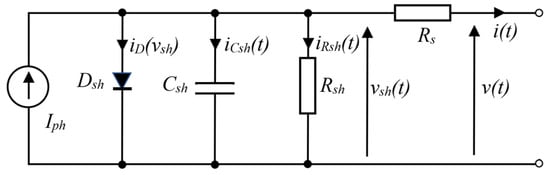
Figure 1. PV panel circuit model.

In Figure 1, D_sh is the p-n junction diode, C_sh is the shunt capacitor for the PN junction, R_sh and R_s are shunt resistor and series resistor, and i_D is the diode current. I_ph is the current source depending on the level of irradiance.

$$i_D\left(v_{sh}\right)=I_o\left(e^{{\displaystyle \frac{v_{sh}}{v_T}}}-1\right)$$

(1)

where

• Reverse saturation current—I_o
• Thermal voltage—v_T = n_id kT/q
• Ideality factor—n_id
• Elementary charge—q
• Boltzmann constant—k
• p-n junction temperature—T

The capacitor current is given by (2), and the output current is given by (3).

$$i_{Csh}=C_{sh}{\displaystyle \frac{d{v}_{sh}}{dt}}=I_{ph}-i_D-{\displaystyle \frac{v_{sh}}{R_{sh}}}-{\displaystyle \frac{v-v_{sh}}{R_s}}$$

(2)

The parameters, voltage and current time-series vectors and current prediction error are defined as follows:

• Parameter vector—P = [I_ph I_o V_T R_sh C_sh R_s]
• Output voltage vector—V = [v[0], v[1], …, v[N]]
• Output current vector—I = [i[0], i[1], …, i[N]]
• Capacitor voltage vector—V_sh = [v_sh[0],v_sh[1], …, v_sh[N]]
• Predicted output current—I_p = [i_p[0],i_p[1], …, i_p[N]]

The current prediction error E_p is given by Equation (3).

$$E_p={\displaystyle \frac{1}{N}}({\mathbf{I}}_{\mathbf{p}}-\mathbf{I}){{(\mathit{I}}_{\mathit{p}}-\mathit{I})}^T={\displaystyle \frac{1}{N}}{\sum }_{k=1}^N{\left(i_p\left[k\right]-i\left[k\right]\right)}^2$$

(3)

An external load perturbation is injected into the output of the solar panel. In this study, the output load voltage or current can be fixed by the electronic load at the output of the solar panel. If the output voltage is fixed by the electronic load with a sinusoidal waveform, as shown in Figure 2, the output current is predicted by the parameter vector P, and the current prediction error can be determined. On the other hand, if the output load current is fixed by the electronic load with a sinusoidal waveform, as shown in Figure 2, the output voltage is predicted by the parameter vector, and the voltage prediction error can be determined. Consider the first case with a fixed sinusoidal load voltage; the initial value of i_Csh[0] can be estimated in step 1, and the current prediction procedures are summarized in steps 2 to 5.

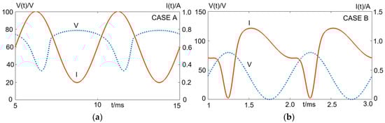
Figure 2. Simulated v(t) and i(t) curves of PV panel. (a) Outputs with fixed sinusoidal load current. (b) Outputs with fixed sinusoidal load voltage.

Step 1: Solve Equation (4) numerically to find v_sh[0] for given i_Csh[0] (e.g., i_Csh[0] = 0), P and v[0].

$$i_{Csh}\left[0\right]=I_{ph}-I_o\left[e^{{\displaystyle \frac{v_{sh}\left[0\right]}{v_T}}}-1\right]-{\displaystyle \frac{v_{sh}\left[0\right]}{R_{sh}}}-{\displaystyle \frac{v_{sh}\left[0\right]-v\left[0\right]}{R_s}}$$

(4)

Step 2: If output voltage v[k] is used as a reference for output current prediction. solve Equations (5) and (6) numerically for given P and V. For k = 0, …, N, perform steps 2–4 to update dv_sh[k]/dt and i_p[k].

$$i_p\left[k\right]={\displaystyle \frac{v_{sh}\left[k\right]-v\left[k\right]}{R_s}}$$

(5)

$${\displaystyle \frac{d{v}_{sh}\left[k+1\right]}{dt}}={\displaystyle \frac{1}{C_{sh}}}\left[I_{ph}-I_o\left[e^{{\displaystyle \frac{v_{sh}\left[k\right]}{v_T}}}-1\right]-{\displaystyle \frac{v_{sh}\left[k\right]}{R_{sh}}}-i_p\left[k\right]\right]$$

(6)

Step 3: Update the v_sh[k] using Equation (7)

$$v_{sh}\left[k+1\right]=v_{sh}\left[k\right]+{\displaystyle \frac{d{v}_{sh}\left[k+1\right]}{dt}}\Delta t$$

(7)

Step 4: Determine the current prediction error E_p using Equation (3)

Step 5: Go back to step 2 until k = N.

For the second case with fixed sinusoidal load current, the output current will be used as a reference for output voltage prediction. Equation (8) is used to estimate the initial value of v_sh[0] for given i_Csh[0], P and i[0]. Equations (9) and (10) are used to update the voltage v_p[k], v_sh[k] and the voltage prediction error E_p.

$$i_{Csh}\left[0\right]=I_{ph}-I_o\left[e^{{\displaystyle \frac{v_{sh}\left[0\right]}{v_T}}}-1\right]-{\displaystyle \frac{v_{sh}\left[0\right]}{R_{sh}}}-i[0]$$

(8)

$$\begin{gathered} {\displaystyle \frac{d{v}_{sh}\left[k+1\right]}{dt}}={\displaystyle \frac{1}{C_{sh}}}\left[I_{ph}-i_D\left[k\right]=I_o\left[e^{{\displaystyle \frac{v_{sh}\left[k\right]}{v_T}}}-1\right]-{\displaystyle \frac{v_{sh}\left[k\right]}{R_{sh}}}-i\left[k\right]\right]; \\ {v}_p\left[k\right]=v_{sh}\left[k\right]-i\left[k\right]R_s \end{gathered}$$

(9)

$$E_p={\displaystyle \frac{1}{N}}\sum _{k=1}^N{\left(v_p\left[k\right]-v\left[k\right]\right)}^2$$

(10)

2.2. Proposed System Structure

Figure 3 shows the proposed PV model parameter estimation system. A load perturbation is injected at the output of the PV panel, and the output voltage and current are sampled and measured. The measured current and voltage vectors are used as inputs to the Model Parameter Classifier (MPC). The MPC is an ANN with two hidden layers (No. of input nodes N_i = 100, N₁ = 200, N₂ = 100, No. of output nodes N_o = 6), which was trained to estimate the range of the model parameters based on the current and voltage vectors. The MPC is designed to approximate the mapping R = φ(P) between the current–voltage input vectors (V = [v[0], …, v[49]], I = [i[0], …, i[49]]) and the range index vector R = [γ₁ γ₂ γ₃ γ₄ γ₅ γ₆] of the model parameters P = [I_ph I_o V_T R_sh C_sh R_s], where γ_i is the index value for p_i, γ_i ∈ {1,2…N_r} and (γ_i − 1)Δp_i/N_r ≤ p_i ≤ γ_i Δp_i/N_r, Δp_i = p_imax − p_imin. The values p_imax and p_imin are the maximum and minimum values of the ith parameter, and N_r is the number of partitions (5 ≤ N_r ≤ 10) for γ_i.

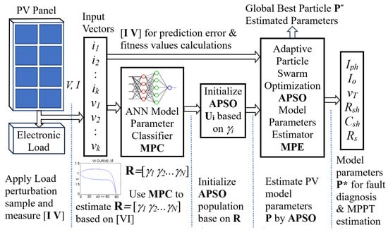
Figure 3. Proposed PV model parameter estimation system.

Since R = [γ₁ γ₂ γ₃ γ₄ γ₅ γ₆] and γ_i ∈ {1,2…N_r}, there will be a total number of (N_r)⁶ combinations or patterns in the set of R. Each index vector R encodes the model parameter P = [I_ph I_o V_T R_sh C_sh R_s] = [p₁ p₂ p₃ p₄ p₅ p₆] as a label from which we can identify the range γ_i of each parameter value p_i. The MPC functions as a classifier to identify the label R according to the IV pattern. For training the MPC, a training dataset {I,V,R} is generated by the simulated models with each model parameter p_i fluctuating within the minimum p_imin and maximum p_imax design values. The parameter range index (γ_i) of the model parameter p_i is determined by γ_I = trunc{[p_i − p_imin]/[p_imax − p_imin]N_r} and the range vector R_i = [γ₁ γ₂ γ₃ γ₄ γ₅ γ₆] can be formed. The load voltage V and current I vectors are generated by a PV simulated model. The dc offset and amplitude of the sinusoidal load voltage or load current are chosen to ensure that the variation in output voltage and current is positive and within the practical limits (V_max ≥ V ≥ 0 and I_max ≥ I ≥ 0, 0–3 A, 0–80 V), as shown in Figure 4. The IV curves are generated for different model parameter vectors, and Figure 4 shows the fluctuating region of the generated IV curves. The generated IV dataset is separated into two parts, in which 80% is used as the ANN training dataset and 20% is used as the testing set. The training algorithms for MPC are implemented by using Python (Library used: numpy 1.23.4, pytorch 1.8.2, pyswarms 1.3.0). The MPC is used to estimate the model parameter range vector R based on the IV input vectors {I, V}. The population for APSO algorithms is then initialized according to the results of MPC (i.e., p_i is chosen randomly within the range γ_i (γ_i − 1)Δp_i/N_r ≤ p_i ≤ γ_i Δp_i/N_r, Δp_i = p_imax − p_imin). The APSO algorithm is used as a model parameter estimator in Figure 3 to estimate the optimal PV panel model parameter P*. Furthermore, the voltage for the maximum power point (MPPT) can also be estimated based on the estimated PV panel model parameter P* (Appendix A).

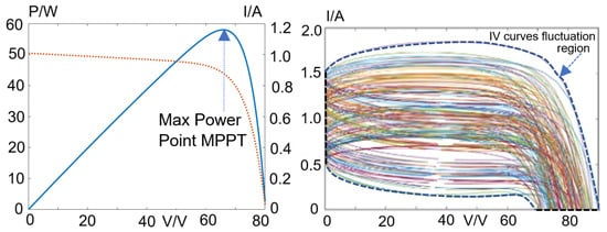
Figure 4. Example of PV panel V-I curve; variations in VI curve for variations in P.

2.3. Adaptive Particle Swarm Optimization

Adaptive Particle Swarm Optimization (APSO) was proposed in [27]. The parameter (e.g., mean distance for particles) of the population distribution is evaluated every generation, and an evolutionary factor is found. Based on the evolution factor, an evolutionary state estimation algorithm is used to identify the evolution state of the population. The evolutionary state includes exploration, exploitation, convergence and jumping out. The APSO enables adaptive control of the inertia weight, acceleration coefficients and other algorithmic parameters at each generation, and this control method can improve the search efficiency and convergence speed. When the population is in a converegce state, APSO will activiate an elist learning strategy to allow the global best particle jumping out from the current local optimal point to search for a possible new global maximum. The equations for the APSO are as follows.

X_i = [X_i1, X_i2, …, X_ik…X_in]

(11)

V_i = [V_i1,V_i2, …, X_ik…V_in]

(12)

V_ik(t + 1) = ωV_ik(t) + C₁ r_1k (P_ik − X_ik) + C₂ r_2k (P_gk − X_ik)

(13)

X_ik(t + 1) = X_ik(t) + V_ik(t + 1), i = 1…N_p

(14)

$${\Phi }_{xi}={\displaystyle \frac{1}{N}}{\sum }_{j=1}^N{e_j}^2={\displaystyle \frac{1}{N}}{\sum }_{j=1}^N{\left[I_{pj}-I_j\right]}^2$$

(15)

where

• Particle position—X_i = [I_ph(i) I_o(i) V_Ti(i) R_sh(i) C_sh(i) R_s(i)]
• Particle velocity and fitness value—V_i, Φ_xi
• Best position experience of ith particle—P_i
• Best fitness experience of ith particle—Φ_ibest
• Best position experience of the whole swam—P_g
• Best fitness experience of the whole swarm—Φ_gbest
• Inertia weight—ω
• Cognitive and Social acceleration coefficients—C₁ and C₂
• Random numbers in [0, 1]—r_1k and r_2k
• Population size—N_p

2.4. Proposed Method and Procedures

The step-by-step procedures for the proposed PV model parameter estimation method are summarized as follows, and a flowchart is shown in Figure 5.

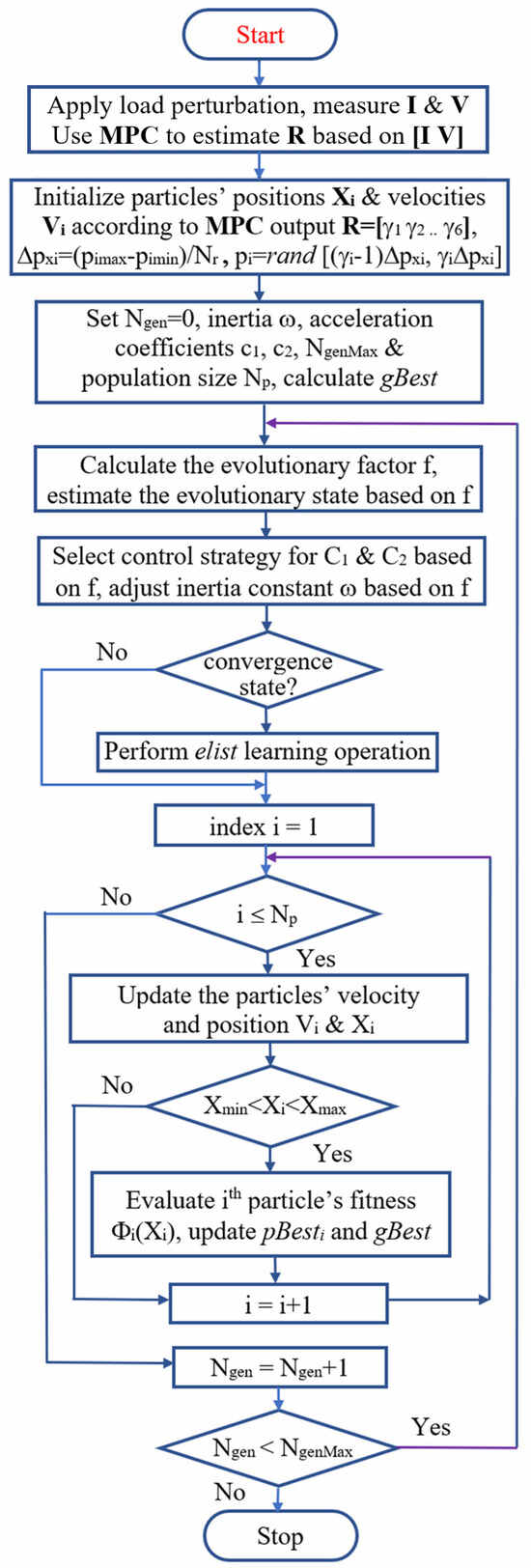
Figure 5. Flowchart of the proposed method.

• Apply a sinusoidal load perturbation to the output of the PV panel; measure and sample the solar panel output voltage and current. Form the current I and voltage V vectors.
• Use the I, V vectors as inputs to the MPC. Estimate the model parameter range vector R = [γ1 γ2 γ3 γ4 γ5 γ6] by using MPC.
• Initialize the population of the APSO algorithm by using R = [γ₁ γ₂ γ₃ γ₄ γ₅ γ₆]. Initialize the components x_i (i = 1…6) of the N_p particles X_i by selecting a random number in the interval [γ_i (Δp_i/N_r), (γ_i + 1)(Δp_i/N_r)], where Δp_i = p_imax − p_imin.
• Using the fitness function Φ_xi = Σ [I_p − I*]²/N (I_p = predicted current, I* = actual current), update the position (X_i = [I_ph I_o V_T R_sh C_sh R_s]) and velocity (V_i) of the particles for i = 1…N_p. Calculate the fitness values for all particles Φ(X_i) for i = 1…N_p.
• Calculate the evolutionary factor f for the population. Estimate the evolution states (exploration, exploitation, convergence, jumping out) of the population by using the Evolution State Estimation algorithm in [27].
• According to the algorithm in [27], select the control strategies for adjustment of cognitive acceleration coefficients C₁ and social acceleration coefficients C₂ based on the evolution state. Apply the adaptive control algorithm on the inertia weight ω based on the evolution factor f.
• If the population is in a convergence state, perform elitist learning operation to allow the global best particle to jump out from the local optimal point.
• Update the velocity V_i and position X_i of all particles. Evaluate the fitness values Φ(X_i) of all particles Xi, and then update the individual best and global best fitness values for the population.
• Repeat steps 4–8. The APSO iterations repeat until the maximum number of generations is reached.
• The global best particle vector X* will be used as the optimal solar panel model parameter vector P*. Furthermore, the voltage for maximum power operation V_p can be estimated by using P*.

3. Results

The ANN–APSO algorithm was implemented on a server with 2.6 GHz Intel CPU i7-8700 (Intel, Santa Clara, CA, USA) and 32 GB memory. The current and voltage vector dataset was generated by the PV panel model [23] in Section 2.1. Two nominal models in Table 1 are considered in simulation studies. The inputs to the MPC consist of 100 entries (V[0]…V[49], i[0]…i[49]). The MPC is an ANN with two hidden layers, with a first hidden layer of 200 nodes, second hidden layer of 100 nodes and output layers of 6 nodes. The learning rate of ANN is 0.01.

Table 1. Nominal model parameters and parameter variations for simulation studies.

Nominal Values	Iph	Io	VT	Rsh	Csh	Rs
Model A	1.00 (±80%)	1 × 10−7 (±80%)	5.00 (±5%)	1000 (±80%)	1 × 10−6 (±80%)	1.00 (±80%)
Model B	2.38 (±90%)	1.45 × 10−7 (±90%)	1.02 (±10%)	118 (±90%)	0.876 × 10−6 (±90%)	0.347 (±90%)

3.1. Simulation Studies

The nominal PV Model A parameters were given ±80% variations, while v_T was given a ±5% variation for generating dataset A. The output voltage is used as a reference for current prediction. Dataset A consisted of 2748 data lines (each line: 50 voltage and 50 current samples), of which 2199 (80%) data lines were used for training and 549 (20%) data lines were used for testing. The settings for the APSO are as follows: maximum number of generations N_max = 200, population size N_p = 20 and particle dimension N = 100. The simulation results of the parameter estimation error (e_i = [p_i − p_i*]/p_i*) and 15 data samples of simulated model parameters are summarized in Table 2. The estimation results are summarized in Table 3 and Figure 6.

Table 2. Model A as nominal model; ANN+APSO average model parameter estimation error for 15 data samples.

Exact Model Parameters						ANN + APSO Parameter Estimation Error (%)						Avg Par
Iph	Io	VT	Rsh	Csh	Rs	Iph	Io	VT	Rsh	Csh	Rs	|Err|%
1.470966	1.29 × 10−7	4.955088	1353.875	1.42 × 10−6	1.541955	0.057%	15.932%	0.918%	−1.128%	−0.400%	−3.025%	3.577%
1.097623	1.07 × 10−7	5.021067	1144.587	5.63 × 10−7	1.056793	0.009%	−2.009%	−0.124%	−0.780%	−0.016%	−0.040%	0.496%
1.450665	1.28 × 10−7	5.038308	1653.205	1.38 × 10−6	1.691926	−0.023%	10.123%	0.594%	3.046%	−0.040%	−1.243%	2.512%
1.048628	1.16 × 10−7	5.029487	1307.631	5.44 × 10−7	1.341587	0.014%	10.569%	0.646%	−3.671%	−0.474%	−5.071%	3.407%
0.554694	1.55 × 10−7	4.986679	1319.290	6.58 × 10−7	1.148153	0.633%	−2.246%	−0.059%	−15.066%	−1.608%	−8.434%	4.674%
1.509694	1.34 × 10−7	4.966657	669.0815	5.69 × 10−7	1.465456	0.061%	17.691%	1.024%	−1.816%	−0.644%	−3.500%	4.123%
0.813365	1.19 × 10−7	5.032863	559.3855	6.04 × 10−7	1.141564	−0.291%	−7.573%	−0.548%	4.988%	1.683%	6.987%	3.678%
0.542401	1.18 × 10−7	5.024342	1493.297	1.38 × 10−6	1.674077	0.041%	−1.571%	−0.098%	−1.215%	−0.012%	−0.012%	0.491%
0.393605	1.30 × 10−7	4.956964	852.0390	4.75 × 10−7	1.678522	−0.325%	10.811%	0.642%	4.872%	0.334%	−0.166%	2.858%
0.480798	1.27 × 10−7	5.028104	753.0568	8.73 × 10−7	1.410295	−0.547%	−3.714%	−0.320%	7.427%	1.465%	6.155%	3.271%
0.562543	1.67 × 10−7	5.013793	547.6574	1.21 × 10−6	1.286810	0.178%	−9.731%	−0.655%	−2.260%	0.015%	0.856%	2.283%
1.318440	1.50 × 10−7	4.993523	470.1839	9.38 × 10−7	0.677297	−1.047%	−2.636%	−0.234%	18.814%	−0.474%	1.893%	4.183%
1.190762	1.52 × 10−7	4.972803	719.7781	1.17 × 10−6	1.154633	−0.398%	2.377%	0.105%	12.182%	0.514%	2.247%	2.971%
0.553598	7.78 × 10−8	5.047605	1050.479	1.30 × 10−6	1.204574	0.383%	−15.138%	−0.988%	−7.481%	−0.107%	−2.033%	4.355%
0.796254	7.98 × 10−8	4.979215	437.8656	1.30 × 10−6	1.154507	−0.313%	7.408%	0.465%	0.653%	−1.177%	−4.274%	2.382%

Table 3. Model A as nominal, average estimation absolute error of the model parameters for different methods.

	Average Absolute Parameter Estimation Error for Dataset A Testing (%)						Overall Average
Model A (Nominal)	Iph	Io	VT%	Rsh	Csh	Rs	Par |Err|%
Variation Range	±80%	±80%	±5%	±80%	±80%	±80%
ANN	6.282%	7.262%	0.410%	10.270%	6.731%	6.462%	6.236%
PSO	0.235%	25.895%	1.613%	6.295%	0.162%	8.426%	7.105%
ANN + PSO	0.056%	11.355%	0.736%	2.532%	0.124%	5.075%	3.313%
ANN + APSO	1.068%	9.394%	0.608%	2.844%	1.081%	2.901%	2.983%

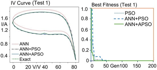
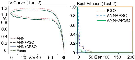
Figure 6. Model A—Samples of PV curves obtained by ANN, ANN + PSO, ANN + APSO and exact model simulations. Test 1: Exact parameters I_ph = 1.451, I_o = 1.28 × 10⁻⁷, V_T = 5.038, R_sh = 1653.205, C_sh = 1.38 × 10⁻⁶, R_s = 1.692. Test 2: Exact parameters I_ph = 1.049, I_o = 1.16 × 10⁻⁷, V_T = 5.029, R_sh = 1307.631, C_sh = 5.44 × 10⁻⁷, R_s = 1.342.

In Table 4 and Figure 7, the nominal PV Model B parameters were given ±90% variations, while v_T was given a ±10% variation for generating dataset B (total 2748 data lines, 80% data lines for training and 20% data lines for testing). The output current is used as a reference for voltage prediction, as described in Section 2.1. The estimation results are summarized in Table 5 and Figure 7.

Table 4. Model B as nominal model—ANN + APSO average model parameter estimation error for 15 data samples.

Exact Model Parameters						ANN + APSO Parameter Estimation Error (%)						Avg Par
Iph	Io	|Err|%	Rsh	Csh	Rs	Iph	Io	VT	Rsh	Csh	Rs	|Err|%
2.098417	2.29 × 10−7	1.906146	151.0366	1.44 × 10−6	0.357008	−0.04%	2.90%	0.17%	0.28%	3.60%	−2.12%	1.52%
2.964697	1.89 × 10−7	1.148021	217.7511	1.71 × 10−6	0.147574	0.17%	−11.39%	−0.72%	−15.10%	17.72%	0.68%	7.63%
2.054445	2.29 × 10−7	1.995245	105.2213	7.59 × 10−7	0.512956	0.45%	−4.01%	−0.40%	−5.23%	2.44%	−10.04%	3.76%
1.793733	2.42 × 10−7	2.021401	171.9073	1.52 × 10−6	0.342945	−0.13%	16.92%	0.92%	1.82%	0.62%	−15.17%	5.93%
4.619483	1.83 × 10−7	1.67785	179.6671	9.80 × 10−7	0.11972	0.38%	−26.44%	−1.82%	1.16%	2.49%	3.56%	5.97%
1.945674	2.37 × 10−7	0.740514	127.5583	1.75 × 10−6	0.475484	0.71%	−3.19%	−0.31%	−18.65%	2.81%	−3.34%	4.83%
2.012295	2.60 × 10−7	1.716977	39.78547	1.12 × 10−7	0.53712	0.09%	3.29%	0.39%	0.37%	0.81%	11.41%	2.73%
2.159246	2.50 × 10−7	1.454867	219.2025	2.21 × 10−7	0.223583	−0.59%	15.19%	1.11%	5.26%	−2.28%	−9.40%	5.64%
2.883559	2.41 × 10−7	1.807694	174.7565	1.78 × 10−6	0.589445	−0.73%	−22.10%	−1.49%	3.61%	−0.34%	0.60%	4.81%
1.858229	1.08 × 10−7	1.976032	204.3552	7.02 × 10−7	0.537653	−0.04%	−25.56%	−1.68%	0.54%	1.12%	8.56%	6.25%
2.099534	2.04 × 10−7	1.776944	204.6018	7.90 × 10−7	0.474764	0.10%	5.81%	0.34%	−1.53%	10.13%	−1.47%	3.23%
2.056924	9.80 × 10−8	1.289721	21.94353	5.91 × 10−7	0.446339	−0.25%	32.69%	1.70%	0.78%	6.27%	−7.99%	8.28%
2.113606	5.22 × 10−8	0.805124	36.86171	1.43 × 10−6	0.537324	−0.19%	37.49%	1.63%	0.93%	1.52%	−7.52%	8.21%
3.856504	2.19 × 10−7	1.526099	15.29461	1.14 × 10−6	0.656692	6.82%	−8.59%	−0.42%	−16.58%	16.48%	−2.71%	8.60%
1.843931	1.19 × 10−7	1.748883	151.2045	1.15 × 10−6	0.244053	−0.16%	30.89%	1.61%	2.90%	0.61%	−13.47%	8.27%

Figure 7. MODEL B—Samples of PV curves obtained by ANN, ANN + APSO and exact model simulations. Test 3: Exact parameters I_ph = 2.098417, I_o = 2.29 × 10⁻⁷, V_T = 1.906146, R_sh = 151.0366, C_sh = 1.44 × 10⁻⁶, R_s = 0.357008. Test 4: Exact parameters I_ph =2.054445, I_o = 2.29 × 10⁻⁷, V_T = 1.995245, R_sh = 105.2213, C_sh = 7.59 × 10⁻⁷, R_s = 0.512956.

Table 5. Model B as nominal model, average estimation absolute error of the model parameters for different methods.

	Average Absolute Parameter Estimation Error for Dataset B Testing (%)						Overall Average
Model B (Nominal)	Iph	Io	VT	Rsh	Csh	Rs	Par |Err| %
Variation Range	±90%	±90%	±10%	±90%	±90%	±90%
ANN	5.920%	8.250%	0.850%	12.270%	8.531%	7.221%	7.17%
PSO	1.311%	13.517%	0.886%	20.168%	1.512%	7.455%	7.48%
ANN + PSO	0.32%	9.44%	1.29%	9.70%	10.39%	8.51%	6.61%
ANN + APSO	0.86%	2.38%	0.61%	1.76%	13.02%	5.89%	4.09%

3.2. Experimental Dataset Analysis

In this study, the experimental dataset in [40] (Sungen SG-NH80-GG 80 W, a-Si type, electronic load HP6050A) is used to evaluate the performances of the proposed algorithm. Experimental I–V data in [40] were inputted to the proposed system, and the estimation results are summarized in Table 6 and Figure 8. The dataset with a high-temperature condition in [40] is used (i.e., the lights were turned ON for 2 min and the panels were heated up). In Table 6, dataset 1 is the data in [40] for sample 1 with cracks, and dataset 2 is the data in [40] for sample 2 with cracks. As there are no reference model parameters for the experimental study, the estimated model parameters are used to predict the current output, and the root mean square error (RMSE) between the estimated and measured values is used as a performance index for comparisons of different methods.

Table 6. Results of parameter estimation, testing of proposed method by the experimental data in [40].

Panel	Predicted Parameter Values by Method in [40]						Iest	Predicted Parameter Values by Proposed ANN + APSO						Iest
	Iph	Io	VT	Rsh	Csh	Rs	RMSE	Iph	Io	VT	Rsh	Csh	Rs	RMSE
Dataset 1	0.602	7.09 × 10−8	5.26	369	2.60 × 10−7	2.60	0.2100	0.5517	2.74 × 10−4	10.832	1826.6	1.42 × 10−6	3.5342	0.0476
Dataset 2	0.454	1.80 × 10−8	5.23	587	4.82 × 10−7	4.82	0.2227	0.434	7.59 × 10−4	13	2119.7	1.40 × 10−6	6.3566	0.1061

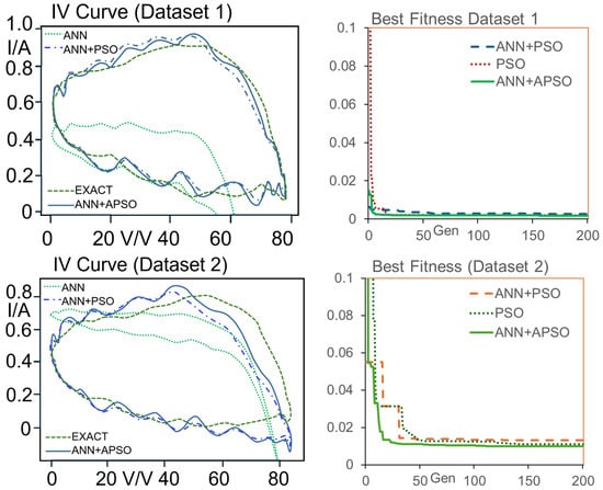
Figure 8. Estimated and measured IV curves; fitness vs. generation for experiment dataset in [40].

3.3. Experimental Studies

A schematic diagram is shown in Figure 9, and the experimental setups are shown in Figure 10. The solar PV panel (SUNGEN SP-50, Shantou, China) is tested under the illumination of the controlled light sources (4× PHILIPS QVF135 HAL-TDS500W 220 V, 50 Hz lamp setup, Shenzhen, China); the outputs of the solar PV panel are connected to the Programmable Electronic Load (CHROMA Electronic Load 63600, Taoyuan, Taiwan). The electronic load draws a sinusoidal load current from the PV panel, as shown in Figure 10, and the voltage and current values are measured and sampled by the software panel of the electronic load. The surface irradiance and temperature of the solar PV panel are measured using a solar irradiance meter (Fluke FLK-IRR1-SOL, Washington, DC, USA). The results of parameter estimations are summarized in Table 7, and the experimental results are summarized in Figure 11.

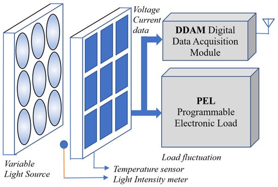
Figure 9. Schematic diagram for experimental studies.

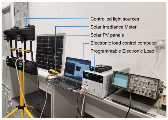
Figure 10. Experimental setup.

Table 7. Results of parameter estimation; testing of proposed method by the experimental setup in Figure 10.

Panel	Predicted Parameter Values by Method in [40]						Iest	Predicted Parameter Values by Proposed ANN + APSO						Iest
	Iph	Io	VT	Rsh	Csh	Rs	RMSE	Iph	Io	VT	Rsh	Csh	Rs	RMSE
Dataset 3	2.38	1.45 × 10−7	1.02	118	8.76 × 10−7	0.347	0.5202	2.390	1.93 × 10−7	1.065	121.82	9.32 × 10−7	0.475	0.2203
Dataset 4	1.86	1.45 × 10−7	1.11	118	1.00 × 10−6	0.348	0.4300	1.870	7.92 × 10−8	1.075	103.28	9.51 × 10−7	0.233	0.1801
Dataset 5	1.16	1.42 × 10−7	1.084	205	2.39 × 10−6	0.702	0.4382	1.19	2.14 × 10−7	1.133	103.48	9.81 × 10−7	0.305	0.0699

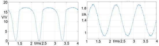
Figure 11. Samples of voltage and current waveforms measured by experiments setup. Electronic load current: 1.4 A dc + 500 Hz sinusoidal (amplitude 0.38 A) AC current.

Testing of Solar PV Panel for Different Irradiance Levels

In experimental studies, the controllable light source is adjusted to give three different levels of irradiance (dataset 3, dataset 4 and dataset 5). The average surface irradiances and temperate are measured for the three tests, and the results are summarized in Table 8. It can be noted that the I_ph is 2.39 for the high irradiance level, 1.87 for medium irradiance level and 1.19 for low irradiance level. It can be noted that the I_ph increases with the level of irradiance. The experimental results are summarized in Figure 12 and Table 9.

Table 8. PV panel surface measurement results.

	Irradiance Level	Average Irradiance (W/m2)	Average Temperature (°C)	Estimated Model Parameter Iph
Dataset 3	High	956.6	36.1	2.39
Dataset 4	Medium	669.8	35.2	1.87
Dataset 5	Low	465.5	34.2	1.19

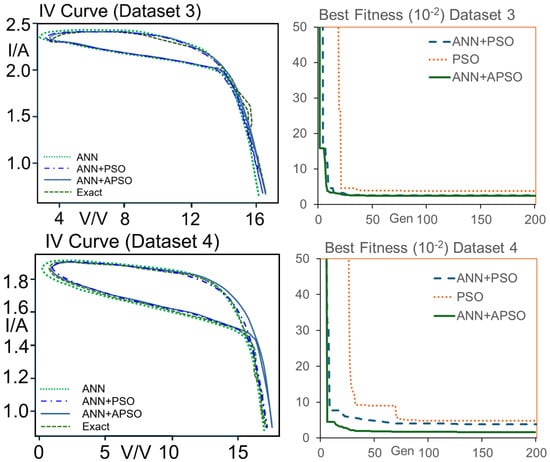
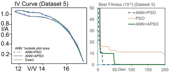
Figure 12. Estimated and measured IV curves; fitness vs. generation for experimental studies in Figure 9 (*ANN is outside plotting range in dataset 5).

Table 9. Summary of different testing results.

Methods	Dataset A Avg|ΔP| err	Dataset B Avg|ΔP| err	Dataset 1 Iest RMSE	Dataset 2 Iest RMSE	Dataset 3 Iest RMSE	Dataset 4 Iest RMSE	Dataset 5 Iest RMSE
ANN	6.236%	7.17%	1.2979	0.4216	0.5202	0.4300	5.4525
PSO	7.105%	7.48%	0.2100	0.2227	0.2738	0.3090	0.4382
ANN + PSO	3.313%	6.61%	0.0555	0.1082	0.2240	0.2753	0.0740
ANN + APSO	2.983%	4.09%	0.0476	0.1061	0.2203	0.1801	0.0699

4. Discussion

4.1. Variation in Model Parameters

In simulation studies, the variation ranges of the model parameters cover the different operating conditions of the solar photovoltaic panel. The magnitude of the current source I_ph of the PV model depends on the level of irradiance. I_ph increases when the irradiance increases. In the simulation studies of Models A and B, the system parameters are given a random variation ±90% of the nominal value, and all the IV curves are generated. The purposes of these parameter fluctuations not only cover the fluctuation in the model parameters due to a change in the operating conditions and health conditions of the solar panel but also cover some simulated PV models for different brands and design specifications. In practical PV panels, the variations in model parameters are well below ±90%. However, the model parameters are purposely given a large variation (±90%) to generate a dataset that covers a parameter variation range smaller than ±90%. As the major function of the MPC is to encode the IV pattern to the range index vector, generating a dataset with a larger range can train the MPC to identify a range index vector for a wide scope of PV model parameter design specifications. It should be noted that partial shading also causes variations in I_ph. According to the studies in [27], I_ph of the cracked panel is smaller than that of the healthy panels. Therefore, I_ph can be used as an indicator for fault occurrence on an open solar farm without shading. It has been found that the variations in C_sh and R_s can indicate a faulty condition with cracked panels. Therefore, the estimated model parameters obtained using the proposed method can be used for fault diagnosis and MPPT tracking.

4.2. Selection of ANN and APSO Parameters

The ANN parameters and the APSO parameters should be selected to achieve optimal results for model parameter estimation. Extensive simulations for the direct ANN model parameter estimator have been conducted. The ANN is used to estimate the six model parameters, with the IV data vector as input. The ANN was trained using the training dataset in Table 1. The simulation results in Table 10 show that the average parameter estimation errors are within ±5% to ±10% when the parameters are given up to ±70% variation. Therefore, a partition number (N_r) of 5 to 10 can match the expected accuracy (±10%) of the MPC. Since the initial estimate of the parameter vector is quite near to the optimal solution, a relatively small APSO population size and a small number of generations are sufficient for the APSO to converge on the optimal solution. Therefore, a population size of 20 is selected, and the maximum number of generations of 200 is selected in this study.

Table 10. Simulation results of model parameter estimation by using direct ANN method.

Model Parameter Variations						Absolute Model Parameter Estimation Error						Avg |ΔPi|
Iph	Io	VT	Rsh	Csh	Rs	Iph	Io	VT	Rsh	Csh	Rs	Error
±50%	±50%	±10%	±50%	±50%	±50%	2.88%	5.12%	0.51%	5.72%	4.36%	7.00%	4.26%
±60%	±60%	±10%	±60%	±60%	±60%	3.82%	8.73%	0.47%	6.79%	4.87%	9.23%	5.65%
±70%	±70%	±10%	±70%	±70%	±70%	5.75%	9.96%	0.49%	9.72%	5.86%	9.93%	6.95%

In order to design the ANN parameters, extensive ANN simulations for the dataset in Table 1 were performed. The loss values for different ANN parameters and hidden node combinations are summarized in Table 11. According to the results in Table 11, a learning rate of 0.01 and a dropout of 0.1 are selected. Furthermore, the loss values for different combinations of hidden nodes are estimated, and the results are summarized in Table 10. In this study, an ANN with two hidden layers, the first hidden layer with 200 nodes (N₁) and the second hidden layer with 100 nodes (N₂), is selected for the MPC. For the selection of APSO meta parameters, the loss values for different combinations of C₁, C₂ ∈ {1.0, 1.5, 2.0} and ω are determined, and the three combinations with loss lower than 0.6 are shown in Figure 13. According to the variation in loss vs. number of generations, the settings C₁ = 1.5, C₂ = 1.5 and ω = 0.1 have the fastest convergence rate, and these settings are used in this study.

Table 11. Selection of learning rate, ANN structure and dropout, PSO settings and loss.

Learning Rate	Loss	ANN Structure	Loss	Nmax = 200, Np = 20,
0.001	0.807	(150,50)	0.854	ω = 0.5
0.005	0.861	(200,100)	0.799	(C1, C2)	Loss
0.01	0.784	(200,150)	0.840	(1.5,1.5)	0.597
0.02	0.830	(200,200)	0.839	(1.5,2)	0.084
0.05	0.799	(300,200)	0.899	(2,1.5)	0.120
0.10	0.830	(200,100,50)	0.817	(C1 = 1.5, C2 = 1.5)
Dropout	Loss	(200,150,50)	0.839	ω	Loss
0.05	0.865	(300,200,100)	0.810	0.2	1090
0.10	0.799			0.5	0.060
0.20	0.843			0.8	2.820

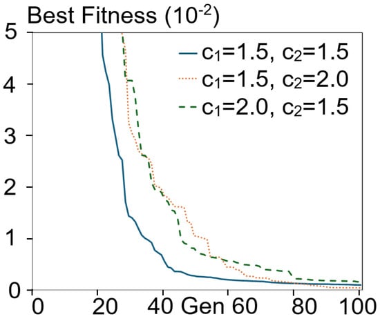
Figure 13. Best fitness vs. number of generations.

4.3. Convergence of Best Fitness

The major purpose of MPC is to estimate the parameter range of the model parameters, and the APSO algorithm is used to finetune the estimated parameters. Since the APSO population is initialized according to the results of MPC, these particle swarms are quite near to the optimal solution; thus, the APSO needs about 200 generations to converge to small fitness values. The variations in the average best fitness vs. number of generations for the Model A test and Model B test (Table 2 and Table 4) for different methods are shown in Figure 14. It can be noted that at 200 generations for the Model A test, the best fitness of PSO, ANN + PSO and ANN + APSO is 0.12, 0.01, and 0.005. Similar results were also obtained from the Model B test; the best fitness of PSO, ANN + PSO and ANN + APSO is 0.1, 0.027 and 0.01 at 200 generations. In general, the convergence rate of ANN + APSO is faster than that of PSO and ANN + PSO. The classical PSO method in [40] will give a small RMSE value of fitness (<5.0) if the number of iterations is greater than 10³.

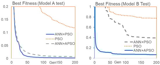
Figure 14. Average best fitness vs. number of generations for Model A and Model B testing.

4.4. Performances of the Proposed Method

According to the results of Model A in Table 2, the average absolute parameter error (APE) for ANN is 6.236%, the average APE for ANN + PSO is 3.313% and the average APE for ANN + APSO is 2.983%. From the results of Model B in Table 4, the average absolute parameter error for ANN is 7.17%, the average APE for ANN + PSO is 6.61% and the average APE for ANN + APSO is 4.09%. It can be seen that ANN + APSO can give a smaller APE within a relatively small number of iterations (N = 200).

From the results of experimental data analysis of dataset 1, the RMSE for the predicted parameters obtained by the method in [40] is 0.21, while the RMSE for the predicted parameters obtained using the proposed method is 0.0476. For the results of dataset 2, the RMSE for the parameters obtained using the method in [40] is 0.2227, and the RMSE for the proposed method is 0.1061. According to the results in [45], the PSO with random particles’ initialization for the PV panel model parameter estimation requires a larger number of iterations (10 × 10³) to reach the steady state, and the overall process requires significant computing resources. On the other hand, the proposed method includes an APSO algorithm with a modified initialization stage.

According to the experimental results of dataset 3 in Section 3.2, the RMSE for the parameters obtained using the method in [40] is 0.52, and the RMSE for the proposed method is 0.22. For the experimental results of dataset 4, the RMSE for the parameters obtained using the method in [40] is 0.43, and the RMSE for the proposed method is 0.1801. For the experimental results of dataset 5, the RMSE for the parameters obtained using the method in [40] is 0.4382, and the RMSE for the proposed method is 0.07. In general, the RMSE of the proposed method is smaller than that of classical PSO [40]. The results in Section 3 show that using the MPC for pre-tuning can speed up the convergence (≈200 iterations) of APSO significantly. The estimation error can reach 5% with a smaller number of iterations.

5. Conclusions

The proposed PV model parameter estimation method gives a smaller parameter estimation error and RMSE (root mean square error) of the predicted current than that of the classical method. The proposed method requires a smaller number of iterations (≈200) to reach the steady state, as compared to classical PSO [40,45]. In this study, the initial particle population is selected according to the pre-tuning results of the MPC. The particles in the initial population should be near to the final optimal solutions, as compared to the random initialization approach. The APSO algorithm is used to estimate the PV panel model parameters, and the proposed method has better performance than that of classical PSO. The proposed algorithm requires less computation power and gives a smaller estimation error than the conventional PSO approach. There is potential to implement the proposed method in a relatively small-scale embedded system. A single-ANN direct approach will give accuracy of about 7.5% for large variation in model parameters. However, when the APSO is used to perform further finetuning of the estimated model parameters, the proposed system can give a small estimation error of less than 5%, and it requires a small population size and a smaller number of iterations to converge to optimal solutions, as compared to classical PSO methods.

References

- Elsheikh, A.H.; Sharshir, S.W.; Elaziz, M.A.; Kabeel, A.E.; Wang, G.; Zhang, H. Modeling of solar energy systems using artificial neural network: A comprehensive review. Sol. Energy 2019, 180, 622–639. [Google Scholar] [CrossRef]
- Saha, C.; Agbu, N.; Jinks, R. Review article of the solar PV parameters estimation using evolutionary algorithms. MOJ Sol. Photoenergy Syst. 2018, 2, 66–78. [Google Scholar] [CrossRef]
- Fahim, S.R.; Hasanien, H.M.; Turky, R.A.; Aleem, S.H.E.A.; Ćalasan, M. A Comprehensive Review of Photovoltaic Modules Models and Algorithms Used in Parameter Extraction. Energies 2022, 15, 8941. [Google Scholar] [CrossRef]
- Mekki, H.; Mellit, A.; Salhi, H.; Khaled, B. Modeling and simulation of photovoltaic panel based on artificial neural networks and VHDL-language. In Proceedings of the ICECS 2007 14th IEEE International Conference on Electronics, Circuits and Systems, Marrakech, Morocco, 11–14 December 2007. [Google Scholar]
- Tina, G.M.; Ventura, C.; Ferlito, S.; De Vito, S. A State-of-Art-Review on Machine-Learning Based Methods for PV. Appl. Sci. 2021, 11, 7550. [Google Scholar] [CrossRef]
- Mellit, A.; Menghanem, M.; Bendekhis, M. Artificial neural network model for prediction solar radiation data: Application for sizing stand-alone photovoltaic power system. In Proceedings of the IEEE Power Engineering Society General Meeting, San Francisco, CA, USA, 16 June 2005; Volume 1, pp. 40–44. [Google Scholar] [CrossRef]
- Mellit, A.; Benghanem, M.; Kalogirou, S.A. Modeling and simulation of a stand-alone photovoltaic system using an adaptive artificial neural network: Proposition for a new sizing procedure. Renew. Energy 2007, 32, 285–313. [Google Scholar] [CrossRef]
- Baptista, D.; Abreu, S.; Travieso-González, C.; Morgado-Dias, F. Hardware implementation of an artificial neural network model to predict the energy production of a photovoltaic system. Microprocess. Microsyst. 2017, 49, 77–86. [Google Scholar] [CrossRef]
- Yona, A.; Senjyu, T.; Saber, A.Y.; Funabashi, T.; Sekine, H.; Kim, C.-H. Application of Neural Network to 24-hour Ahead Generating Power Forecasting for PV System. In Proceedings of the 2008 IEEE Power and Energy Society General Meeting—Conversion and Delivery of Electrical Energy in the 21st Century, Pittsburgh, PA, USA, 20–24 July 2008. [Google Scholar]
- Saberian, A.; Hizam, H.; Radzi, M.A.M.; Kadir, M.Z.A.A.; Mirzaei, M. Modelling and Prediction of Photovoltaic Power Output Using Artificial Neural Networks. Int. J. Photoenergy 2014, 2014, 469701. [Google Scholar] [CrossRef]
- Liu, L.; Liu, D.; Sun, Q.; Li, H.; Wennersten, R. Forecasting Power Output of Photovoltaic System Using A BP Network Method. Energy Procedia 2017, 142, 780–786. [Google Scholar] [CrossRef]
- Mellit, A.; Saglam, S.; Kalogirou, S.A. Artificial neural network-based model for estimating the produced power of a photovoltaic module. Renew. Energy 2013, 60, 71–78. [Google Scholar] [CrossRef]
- Huang, C.-J.; Kuo, P.-H. Multiple-Input Deep Convolutional Neural Network Model for Short-Term Photovoltaic Power Forecasting. IEEE Access 2019, 7, 74822–74834. [Google Scholar] [CrossRef]
- Wang, H.; Yi, H.; Peng, J.; Wang, G.; Liu, Y.; Jiang, H.; Liu, W. Deterministic and probabilistic forecasting of photovoltaic power based on deep convolutional neural network. Energy Convers. Manag. 2017, 153, 409–422. [Google Scholar] [CrossRef]
- Al-Waelia, A.H.A.; Sopiana, K.; Yousifb, J.H.; Kazemb, H.A.; Bolandc, J.; Chaichand, M.T. Artificial neural network modeling and analysis of photovoltaic/thermal system based on the experimental study. Energy Convers. Manag. 2019, 186, 368–379. [Google Scholar] [CrossRef]
- Celik, A.N. Artificial neural network modelling and experimental verification of the operating current of mono-crystalline photovoltaic modules. Sol. Energy 2011, 85, 2507–2517. [Google Scholar] [CrossRef]
- Bonanno, F.; Capizzi, G.; Graditi, G.; Napoli, C.; Tina, G.M. A radial basis function neural network based approach for the electrical characteristics estimation of a photovoltaic module. Appl. Energy 2012, 97, 956–961. [Google Scholar] [CrossRef]
- Karatepe, E.; Boztepe, M.; Colak, M. Neural network based solar cell model. Energy Convers. Manag. 2006, 47, 1159–1178. [Google Scholar] [CrossRef]
- Laudani, A.; Lozito, G.M.; Radicioni, M.; Fulginei, F.R.; Salvini, A. Model Identification for Photovoltaic Panels Using Neural Networks. In Proceedings of the International Conference on Neural Computation Theory and Applications—IJCCI, Rome, Italy, 22–24 October 2014; Volume 3, pp. 130–137. [Google Scholar]
- Salem, F.; Awadallah, M.A. Parameters estimation of Photovoltaic modules: Comparisons of ANFIS and ANN. Int. J. Ind. Electron. Drives 2014, 1, 121–129. [Google Scholar] [CrossRef]
- Dharmarajan, R.; Ramachandran, R. Estimation of PV Module Parameters using Generalized Hopfield Neural Network. Int. Res. J. Multidiscip. Technovation IRJMT 2019, 1, 16–27. [Google Scholar] [CrossRef]
- Elkholy, A.; El-Ela, A.A.A. Optimal parameters estimation and modelling of photovoltaic modules using analytical method. Heliyon 2019, 5, e02137. [Google Scholar] [CrossRef] [PubMed]
- Lo, W.L.; Chung, H.S.H.; Hsung, R.T.C.; Fu, H.; Shen, T.W. PV Panel Model Parameter Estimation by using Neural Network. Sensors 2023, 23, 3657. [Google Scholar] [CrossRef]
- Kennedy, J.; Eberhart, R.C. Particle swarm optimization. In Proceedings of the IEEE International Conference on Neural Networks (ICNN), Perth, Australia, 27 November–1 December 1995; Volume 4, pp. 1942–1948. [Google Scholar]
- Ratnaweera, A.; Halgamuge, S.; Watson, H. Self-organizing hierarchical particle swarm optimizer with time-varying acceleration coefficients. IEEE Trans. Evol. Comput. 2004, 8, 240–255. [Google Scholar] [CrossRef]
- Andrews, P.S. An investigation into mutation operators for particle swarm optimization. In Proceedings of the IEEE Congress on Evolutionary Computation (CEC), Vancouver, BC, Canada, 16–21 July 2006; pp. 1044–1051. [Google Scholar]
- Zhan, Z.-H.; Zhang, J.; Li, Y.; Chung, H.S.-H. Adaptive particle swarm optimization. IEEE Trans. Syst. Man Cybern. Part B Cybern. 2009, 39, 1362–1381. [Google Scholar] [CrossRef]
- Alfi, A. PSO with Adaptive Mutation and Inertia Weight and Its Application in Parameter Estimation of Dynamic Systems. Acta Autom. Sin. 2011, 37, 541–549. [Google Scholar] [CrossRef]
- Kessentini, S.; Barchiesi, D. Particle Swarm Optimization with Adaptive Inertia Weight. Int. J. Mach. Learn. Comput. 2015, 5, 368–373. [Google Scholar] [CrossRef]
- Han, H.; Lu, W.; Qiao, J. An Adaptive Multi-objective Particle Swarm Optimization Based on Multiple Adaptive Methods. IEEE Trans. Cybern. 2017, 47, 2754–2767. [Google Scholar] [CrossRef] [PubMed]
- Li, X.; Mao, K.; Lin, F.; Zhang, X. Particle swarm optimization with state-based adaptive velocity limit strategy. Neurocomputing 2021, 447, 64–79. [Google Scholar] [CrossRef]
- Tian, D.; Liu, C.; Gheni, Z.; Li, B. Adaptive Particle Swarm Optimization based on Competitive and Balanced Learning Strategy. In Proceedings of the 2023 International Conference on Electronics, Computers and Communication Technology—CECCT’23, Guilin, China, 17–19 November 2023; pp. 44–53. [Google Scholar] [CrossRef]
- Dawan, P.; Sriprapha, K.; Kittisontirak, S.; Boonraksa, T.; Junhuathon, N.; Titiroongruang, W.; Niemcharoen, S. Comparison of Power Output Forecasting on the Photovoltaic System Using Adaptive Neuro-Fuzzy Inference Systems and Particle Swarm Optimization-Artificial Neural Network Model. Energies 2020, 13, 351. [Google Scholar] [CrossRef]
- Mughal, M.A.; Ma, Q.; Xiao, C. Photovoltaic Cell Parameter Estimation Using Hybrid Particle Swarm Optimization and Simulated Annealing. Energies 2017, 10, 1213. [Google Scholar] [CrossRef]
- Khelil, K.; Bouadjila, T.; Berrezzek, F.; Khediri, T. Parameter extraction of photovoltaic panels using genetic algorithm. In Proceedings of the Third International Conference on Technological Advances in Electrical Engineering (ICTAEE’18), Beijing, China, 10–12 December 2018. [Google Scholar]
- Ebrahimi, S.M.; Salahshour, E.; Malekzadeh, M.; Gordillo, F. Parameters identification of PV solar cells and modules using flexible particle swarm optimization algorithm. Energy 2019, 179, 358–372. [Google Scholar] [CrossRef]
- Rezk, H.; Arfaoui, J.; Gomaa, M.R. Optimal Parameter Estimation of Solar PV Panel Based on Hybrid Particle Swarm and Grey Wolf Optimization Algorithms. Energy Rep. 2022, 8, 12282–12301. [Google Scholar] [CrossRef]
- Jlidi, M.; Hamidi, F.; Barambones, O.; Abbassi, R.; Jerbi, H.; Aoun, M.; Karami-Mollaee, A. An Artificial Neural Network for Solar Energy Prediction and Control Using Jaya-SMC. Electronics 2023, 12, 592. [Google Scholar] [CrossRef]
- Gupta, J.; Hussain, A.; Singla, M.K.; Nijhawan, P.; Haider, W.; Kotb, H.; AboRas, K.M. Parameter Estimation of Different Photovoltaic Models Using Hybrid Particle Swarm Optimization and Gravitational Search Algorithm. Appl. Sci. 2023, 13, 249. [Google Scholar] [CrossRef]
- Lo, W.-L.; Chung, H.S.-H.; Hsung, R.T.-C.; Fu, H.; Shen, T.-W. PV Panel Model Parameter Estimation by Using Particle Swarm Optimization and Artificial Neural Network. Sensors 2024, 24, 3006. [Google Scholar] [CrossRef]
- Touabi, C.; Ouadi, A.; Bentarzi, H. Photovoltaic Panel Parameters Estimation Using an Opposition Based Initialization Particle Swarm Optimization. Eng. Proc. 2023, 29, 16. [Google Scholar]
- Ramaprabha, R.; Gothandaraman, V.; Kanimozhi, K.; Divya, R.; Mathur, B.L. Maximum power point tracking using GA-optimized artificial neural network for Solar PV system. In Proceedings of the 2011 1st International Conference on Electrical Energy Systems, Chennai, India, 3–5 January 2011; pp. 264–268. [Google Scholar] [CrossRef]
- Shang, L.; Zhu, W.; Li, P.; Guo, H. Maximum power point tracking of PV system under partial shading conditions through flower pollination algorithm. Prot. Control Mod. Power Syst. 2018, 3, 38. [Google Scholar] [CrossRef]
- Ansari, M.F.; Thakur, P.; Saini, P. Particle Swarm Optimization Technique for Photovoltaic System. Int. J. Recent Technol. Eng. IJRTE 2020, 8, 1448–1451. [Google Scholar] [CrossRef]
- Wang, W.; Liu, A.C.-F.; Chung, H.S.-H.; Lau, R.W.-H.; Zhang, J.; Lo, A.W.-L. Fault Diagnosis of Photovoltaic Panels Using Dynamic Current–Voltage Characteristics. IEEE Trans. Power Electron. 2016, 31, 1588–1599. [Google Scholar] [CrossRef]
Disclaimer/Publisher’s Note: The statements, opinions and data contained in all publications are solely those of the individual author(s) and contributor(s) and not of MDPI and/or the editor(s). MDPI and/or the editor(s) disclaim responsibility for any injury to people or property resulting from any ideas, methods, instructions or products referred to in the content. |
© 2025 by the authors. Licensee MDPI, Basel, Switzerland. This article is an open access article distributed under the terms and conditions of the Creative Commons Attribution (CC BY) license (https://creativecommons.org/licenses/by/4.0/).