Improved Decentralized Fractional-Order Control of Higher-Order Systems Using Modified Flower Pollination Optimization

Abstract

Due to increased complexity and interactions between various subsystems, higher-order MIMO systems present difficulties in terms of stability and control performance. This study effort provides a novel, all-encompassing method for creating a decentralized fractional-order control technique for higher-order systems. Given the greater number of variables that needed to be optimized for fractional order control in higher-order, multi-input, multi-output systems, the modified flower pollination optimization algorithm (MFPOA) optimization technique was chosen due to its rapid convergence speed and minimal computational effort. The goal of the design is to improve control performance. Maximum overshoot (Mp), rising time (tr), and settling time (ts) are the performance factors taken into consideration. The MFPOA approach is used to improve the settings of the proposed decentralized fractional-order proportional-integral-derivative (FOPID) controller. By exploring the parameter space and converging on the best controller settings, the MFPOA examines the parameter space and satisfies the imposed constraints by maintaining system stability. To evaluate the suggested approach, simulation studies on two systems are carried out. The results show that by decreasing the loop interactions between subsystems with improved stability, the decentralized control with the MFPOA-based FOPID controller provides better control performance.

1. Introduction

The proportional-integral-derivative (PID) controller was initially conceived in the 1920s and has since gained widespread use. Although numerous other control strategies have been put out over the past 100 years, PID remains the most widely used process control technology in the industrial domain. This is due to the fact that an integer order is used to model most systems. The PID controller offers reliable performance and an easy-to-implement structure at the same time. Additionally, numerous potential methods for adjusting the PID controller’s parameters have been documented in the literature. Nonetheless, in certain scenarios, the system can and ought to be represented as a non-integer-order system; representing the system as an integer order is merely a rough approach [1]. A system that is modeled as a fractional order will be a better approach. Fractional-order control will undoubtedly work better for fractional-order systems.

A sophisticated control method that has gained substantial popularity recently is the fractional-order proportional-integral-derivative (FOPID) controller [2,3]. The FOPID controllers have a higher degree of freedom and greater flexibility due to their additional parameters, which are fractional-order in the integral and derivative terms. The FOPID controller has many benefits when compared with a PID controller. This includes enhanced set-point tracking, strong disturbance rejection, and greater processing ability to withstand model uncertainties [4]. The FOPID controller is appropriate for a variety of applications because it can more precisely capture the dynamic behavior of complex systems when fractional order is used in integrals and derivatives [5]. The FOPID controller has benefits like higher tracking performance, increased stability margins, and robustness to uncertainty. The FOPID controller offers a promising foundation for improving the performance of control systems and overcoming the difficulties posed by complex, nonlinear systems. The foundations of the FOPID controller and its applications are examined in this paper. Along with the most recent advancements and research trends in the area, several techniques for adjusting the FOPID controller parameters are also explored.

Multi-input, multi-output (MIMO) systems are extensively used in the process control sector. Designing an effective controller is challenging due to the interactions between the loops. For the conventional single-input, single-output (SISO) proportional-integral-derivative (PID) controller, a number of tuning techniques are offered [6]. The design approaches that should be taken into account when designing fractional controllers are also outlined.

To achieve the required performance and stability, FOPID controller parameters must be properly selected, which is a significant cause for concern. Model-based and model-free tuning techniques are the two categories into which FOPID controller tuning approaches are categorized in the literature. Several research works have been conducted to provide effective model-based tuning rules and techniques for FOPID controllers [7]. Trajectory tracking of a rotating flexible-joint system was assessed using a state feedback-based fractional integral control approach [8]. For a rotary inverted pendulum, a two-degree-of-freedom FOPID controller was used [9]. In [10], the topic of tuning FO controllers for industrial use was examined. However, for complicated nonlinear systems, these approaches require a precise dynamic model, which is not accessible [11,12]. Conversely, no model or process identification is present in model-free tuning techniques [11]. As a result, ref. [13] looked into the model-free tuning technique for FOPID controlling. In [14], when the characteristics of the system varied over time, a model-free adaptive FOPID tuning technique was applied.

Machine learning techniques are one type of model-free tuning that may be used to properly tune the parameters of the FOPID controller without requiring previous knowledge of the dynamics of the system [15,16]. Neural networks (NNs) were designed to tune the FOPID controller for numerous applications because of their capacity to tune more useful controller settings without requiring a thorough understanding of the system [16].

Although there are many methods for figuring out the FOPID parameters, as described in the aforementioned literature, robustness and stability must be taken into account. Also, figuring out the best controller gains is crucial. Through a tuning approach, the best controller gain values that meet these requirements can be found. Finding the ideal values, however, is the main objective. Numerous studies have examined the tuning of FOPID parameters using metaheuristic optimization methods [17,18,19]. These tuning techniques are actually offline systems and do not rely on the precise mathematical model that represents plants. In this sense, one of the following methods has been utilized to build the FOPID controller: hybrid optimization [20], fuzzy logic [21], particle swarm optimization (PSO) [22], or genetic algorithms [23]. Due to its quicker convergence, PSO-based design is one of the most popular among them, yet it frequently displays a local solution. On the other hand, the global solution achieved by genetic algorithms comes at a great computing expense. Consequently, additional efforts have been undertaken to suggest a different algorithm in order to attain both a global solution and speedier convergence. Different modified flower pollination optimization algorithms (MFPOAs) have been applied recently to solve many engineering optimization problems [24]. The classical flower pollination algorithm (FPA), which was developed to address global optimization based on the imitation of flower pollination, has proven effective in solving a number of optimization problems [25]. Sadly, however, due to its low convergence speed and inability to explore multiple regions within the search space during the optimization process, the classical FPA’s performance still significantly suffers from stagnation in local minima, requiring multiple iterations to find better solutions within unpromising regions. In general, ten mathematical test functions were used to evaluate the classical FPA with a population size of 25, and the maximum iteration reached 10,840. This is regarded as a considerable rate to be consumed in order to get the required results. More details regarding the drawbacks associated with the classical FPA are discussed in [26,27]. This paper adopted the MFPOA presented in [28]. The main benefit of the suggested MFPOA is that the algorithm converges more quickly while maintaining the same properties of the traditional FPA. The MFPOA is one of many nature-inspired algorithms that have been created recently for solving the optimization problem.

This work makes use of the decentralized FOPID controller design for higher-order systems that use the MFPOA. Because of its scalability, fault tolerance, modularity, design simplicity, etc., decentralized control is recommended. To establish the best FOPID controller gains, the MFPOA approach is used. For higher-order systems, the efficiency of the controller can be confirmed by taking parameter fluctuations and disturbances into account. The comparative results show that the suggested controller can meet design requirements with little overshoot and settling time, hence assuring robust stability. The main contributions of the present study are listed as follows:

• Loop interactions and coupling effects are decreased by creating decouplers with a simplified decoupling approach;
• In order to obtain the best values of Ts, Tr, and Mp, a novel optimal FOPID controller is designed using an MFPOA method that places constraints on ITSE. This strengthens the system and improves the stability issues;
• A quantitative comparison is made between the suggested method and the traditional PID controller. The results show that the recommended controller performs better than the previously discussed approaches.

The paper is structured as follows: Section 2 describes the background of decentralized control. Section 3 describes the optimization methodology: classical FPA, MFPOA, and implementation of the MFPOA for optimizing the FOPID controller and proposed cost function. The robust stability analysis is discussed in Section 4. Section 5 presents the simulations results and discussion. Finally, Section 6 presents our conclusions and future work.

2. The Preliminary Background of the Proposed Control Method

This section provides a description of the work’s preliminary steps. The MIMO system’s transfer function with n-input and n-output can be written as

$$M\left(s\right)=\left[\begin{array}{cc}\begin{array}{cc}{m}_{11}\left(s\right)e^{-{\phi }_{11}\left(s\right)}& m_{12}\left(s\right)e^{-{\phi }_{12}\left(s\right)}\\ m_{21}\left(s\right)e^{-{\phi }_{21}\left(s\right)}& m_{22}\left(s\right)e^{-{\phi }_{22}\left(s\right)}\end{array}& \begin{array}{cc}\dots & m_{1n}\left(s\right)e^{-{\phi }_{1n}\left(s\right)}\\ \dots & m_{21}\left(s\right)e^{-{\phi }_{2n}\left(s\right)}\end{array}\\ \begin{array}{cc}\dots & \dots \\ m_{n1}\left(s\right)e^{-{\phi }_{n1}\left(s\right)}& m_{n2}\left(s\right)e^{-{\phi }_{nn}\left(s\right)}\end{array}& \begin{array}{cc}\dots & \dots \\ \dots & m_{nn}\left(s\right)e^{-{\phi }_{nn}\left(s\right)}\end{array}\end{array}\right]$$

(1)

Equation (1) makes clear how the process variables interact with one another. The loop interactions must be reduced in order to meet the design objectives. It has been stated in [29], interactions can be reduced using either a centralized or decentralized controller. However, given its advantages, the decentralized structure is favored. The independent controller is

$$C\left(s\right)=\left[\begin{array}{c}\begin{array}{cccc}{C}_{11}\left(s\right)& 0& 0& 0\\ .& C_{22}\left(s\right)& .& .\\ \dots & \dots & \dots & \dots \\ 0& 0& 0& C_{nn}\left(s\right)\end{array}\end{array}\right]$$

(2)

Figure 1 shows the overall layout of the $3\times 3$ MIMO system with a decentralized controller. First, second, and third loop effects are depicted in blue, green, and red, respectively. It is clear from the figure that loop interactions are a frequent occurrence in MIMO systems. The second and third loops’ effects on the first loop are viewed as a disturbance that needs to be lessened in order to meet the design criteria. The second and third loops operate similarly. By creating decouplers, the loop interactions are reduced to a minimum.

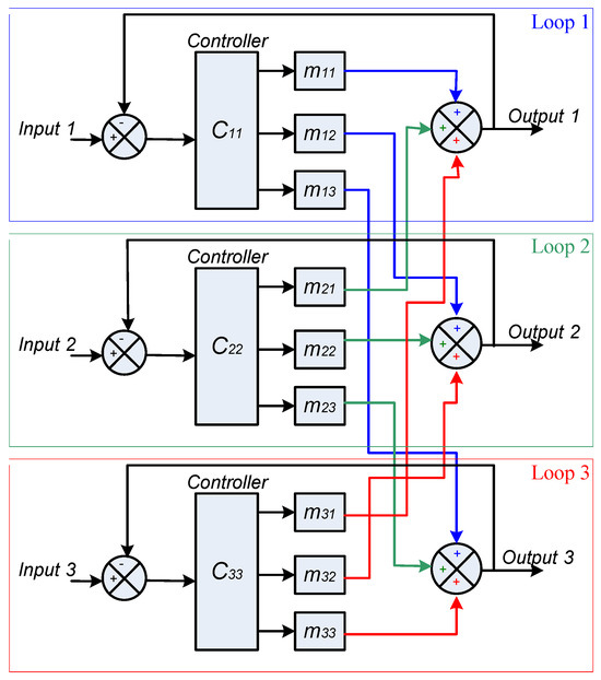
Figure 1. 3 × 3 MIMO system with a decentralized controller.

Figure 2 shows the MIMO system’s schematics with a decoupler and controller. The decouplers basically reduce the interactions between the control loops.

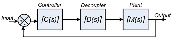
Figure 2. Decentralized control.

In addition, the control law is implemented to meet the appropriate operational standards. Rajapandiyan and Chidambaram [30] state that the decoupling matrix is

$$D\left(s\right)=\left[\begin{array}{c}\begin{array}{cccc}1& -\frac{m_{12}\left(s\right)}{m_{11}\left(s\right)}{e}^{\left(-{\phi }_{12}-{\phi }_{11}\right)s}& \dots & -\frac{m_{1m}\left(s\right)}{m_{11}\left(s\right)}{e}^{\left(-{\phi }_{1m}-{\phi }_{11}\right)s}\\ -\frac{m_{21}\left(s\right)}{m_{22}\left(s\right)}{e}^{\left(-{\phi }_{21}-{\phi }_{22}\right)s}& 1& \dots & -\frac{m_{2m}\left(s\right)}{m_{22}\left(s\right)}{e}^{\left(-{\phi }_{2m}-{\phi }_{22}\right)s}\\ \dots & \dots & \dots & \dots \\ -\frac{m_{m1}\left(s\right)}{m_{mm}\left(s\right)}{e}^{\left(-{\phi }_{m1}-{\phi }_{mm}\right)s}& -\frac{m_{m2}\left(s\right)}{m_{mm}\left(s\right)}{e}^{\left(-{\phi }_{m2}-{\phi }_{mm}\right)s}& \dots & 1\end{array}\end{array}\right]$$

(3)

Consequently, the diagonal matrix $J\left(s\right)$ can be calculated as

$$J\left(s\right)=M\left(s\right)\ast C\left(s\right)=diag\left\{j_{11}\left(s\right),j_{22}\left(s\right),\dots ,j_{mm}\left(s\right)\right\}$$

(4)

For $1=1, 2,$ the decoupled elements $j_{ii}$ need to be controlled.

The higher-order system’s complexity is shown in Equation (1). Additionally, the analysis gets more difficult as the system’s rank rises. As a result, model reduction is preferred because controller design is challenging. The FOPDT model can be used to approximate the process dynamics though. As a result, the structure of the FOPDT model is determined using the proper model-reduction procedures. This model makes it simple to determine the gain, dead time, and time constant [31]. The scaled-down model is

$$M_{ii}\left(s\right)=\frac{W_{ii}{e}^{-{\mathrm{\varnothing }}_{ii}\left(s\right)}}{{\tau }_{ii}s+1},j=\mathrm{1,2}$$

(5)

The unknowns are identified using frequency-response fitting at two positions, $\left(0,{\alpha }_{cii}\right)$ (0, cii), where ${\alpha }_{cii}$ is the phase-crossover frequency.

$$M_{ii}\left(0\right)=j_{ii}\left(0\right)$$

(6)

$$\left|M_{ii}\left(j{\alpha }_{cii}\right)\right|=\left|j_{ii}\left(j{\alpha }_{cii}\right)\right|$$

(7)

$$\mathrm{\angle }\left\{M_{ii}\left(j{\alpha }_{cii}\right)\right\}=\mathrm{\angle }\left\{j_{ii}\left(j{\alpha }_{cii}\right)\right\}$$

(8)

The FOPDT specifications are provided by

$$W_{ii}=\mathrm{s}{j}_{ii}\left(0\right)$$

(9)

$${\tau }_{ii}=\sqrt{\frac{W_{ii}^2-{\left|j_{ii}\left(j{\alpha }_{cii}\right)\right|}^2}{{\left|j_{ii}\left(j{\alpha }_{cii}\right)\right|}^2{\alpha }_{cii}^2}}$$

(10)

$${\mathrm{\varnothing }}_{ii}=\frac{\pi +{tan}^{-}(-{\alpha }_{cii}{\tau }_{ii})}{{\alpha }_{cii}{\tau }_{ii}}$$

(11)

2.1. Fractional Calculus Definitions

Fractional derivatives include the Caputo and Riemann–Liouville (RL) types. All of them are extensions of the standard differential and integral operators. Nonetheless, the features of the fractional derivatives are less than those of the comparable classical ones. Because of this, these derivatives are highly helpful in explaining the abnormal happenings [32,33]. This study makes use of the RL derivative, one of the most often utilized fractional derivatives. The RL derivative outperforms Caputo in that it permits the function in question to have discontinuity at the origin. However, it prohibits the use of conventional initial conditions; instead, the initial conditions in the RL case must either be weighted initial conditions or in the integral form. More numerical aspect/advantages can be found in [34,35,36].

The FO controllers are described by differential equations with fractional-order integrals and derivatives. An FO operator $v{B}_t^x$ is denoted by the following:

$$B_t^x=\left\{\begin{array}{c}\frac{dx}{dt}, R\left(x\right)>0\\ 1, R\left(x\right)=0\\ {\int }_b^t{\left(d\lambda \right)}^{-x}, R\left(x\right)<0\end{array}\right.$$

(12)

with $x\in \mathbb{R}$. According to Garrappa et al. [31], the three definitions for fractional derivatives that are most frequently employed are the Caputo definition, the Riemann–Liouville definition, and the Grunwald–Letnikov definition. However, the Riemann–Liouville definition is more common and is given by

$$v{B}_t^{x}f\left(x\right)=\frac{1}{\gamma (m-x)}\frac{d^a}{d{t}^a}{\int }_l^u\frac{f\left(x\right)}{{(t-\tau )x}^{-a+1}}dx, a-1<x<a$$

(13)

where $\gamma (.)$ stands for the Euler gamma function, and $l$ and $u$, respectively, are the lower and upper bounds. The order of the integral or derivative is $x$, which could be a complex number or a non-integer, and $v{B}_t^x$ is the fractional differentiation or integration. To determine the transfer-function of integer-order systems, the Laplace transform is used. The signal’s $a^{th}$ order derivative’s Laplace transformation is $x\left(t\right)$.

$$\mathcal{L}{B}^{a}x\left(t\right)={\int }_0^{\mathrm{\infty }}{e}^{-st}{}_0{}^{.}{B}_t^{a}x\left(t\right)dt=S^{a}X\left(s\right)-{\sum }_{k=0}^{-1}{s}^k{}_0{}^{.}{B}_t^{n-k-1}{\left.x\left(t\right)\right|}_{t=0}$$

(14)

with $(m-1)<a<m$ and $m\in Z$ as explained in [37]. One method to be applied in simulations, models, or controllers is to approximate fractional orders with integer-order transfer functions. To replicate a fractional transfer function accurately, an integer-order transfer function must have an unlimited number of poles and zeros. However, a finite number $\left(N\right)$ of zeros and poles allows for reliable estimation. The Oustaloup strategy, which takes advantage of the recursive distribution of zeros and poles, is one of the many well-known approximation techniques. The deeper analysis and optimal continuous approximation Oustaloup method can be found in [38,39,40]. The transfer function in the Oustaloup method is written as

$$s^v\approx k{\prod }_{n=1}^N\frac{1+\left(s/v_{z,a}\right)}{1+\left(s/v_{p,a}\right)}$$

(15)

In $\left[{\omega }_1,{\omega }_h\right]$, the approximation is defined. To guarantee that Equation (15) will have a unity gain at 1 rad/s, gain k is modified. The order of approximation affects the chosen value of N. Gain and phase ripples are the results of low-order approximations. With a higher order of N, ripples can be eliminated; however, the computing process is very challenging. Equation (15) describes the frequencies of zeros and poles, which are given by

$${\omega }_{z,l}={\omega }_l\sqrt{\beta }$$

(16)

$${\omega }_{p,a}={\omega }_{z,}\zeta , a=1,\dots ,A$$

(17)

$${\omega }_{z,a+1}={\omega }_{p,a,} a=1,\dots ,A-1$$

(18)

$$\zeta ={\left({\omega }_h/{\omega }_l\right)}^{v/A}$$

(19)

$$\beta ={\left({\omega }_h/{\omega }_l\right)}^{\left(1-v\right)/A}$$

(20)

To take into account the condition $v<0$, Equation (15) might be reversed. If $\left|v\right|>1$, which typically leads to distinct fractional orders as seen below, the approximation becomes unacceptable.

$$s^v=s^a{s}^{\delta }, a\zeta Z, \delta \zeta \left[\mathrm{0,1}\right]$$

(21)

2.2. Stability of the Fractional-Order System

Stability assurance is a fundamental and crucial criterion for constructing a control system. The linear-time-invariant (LTI) system is stable because the roots of the characteristic equation are on the left side of the S plane.

Lemma 1

[41,42]. Let us consider the following autonomous system:

$$\frac{d^{\alpha }x}{d{t}^{\alpha }}=Ax, x\left(0\right)=x_0$$

(22)

where  $0<\alpha <1$, $A\in {\mathit{R}}^{n\times n}$ and $x\in {\mathit{R}}^n$, it is asymptotically stable if and only if  $\left|arg\left(\lambda \right)\right|>\frac{\alpha \pi }{2}$ is fulfilled for each of the matrix A’s eigenvalues (λ). Also, this system is stable if and only if $\left|arg\left(\lambda \right)\right|\ge \frac{\alpha \pi }{2}$ is fulfilled for each of the matrix A’s eigenvalues (λ) with those critical eigenvalues satisfying  $\left|arg\left(\lambda \right)\right|=\frac{\alpha \pi }{2}$ possessing a geometric multiplicity of one. A matrix A’s geometric multiplicity of an eigenvalue λ is its dimension within the subspace of vectors v that satisfy

$$Av=\mathsf{\lambda }v.$$

(23)

Figure 3 depicts the stable and unstable regions for 0 < α < 1.

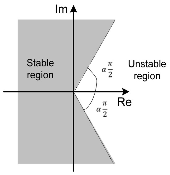
Figure 3. Stability regions of fractional-order systems $0<x<1$.

2.3. Fractional-Order PID (FOPID)

The fractional-order PID (FOPID) controller is an improved version of the PID controller that integrates fractional-order calculus. The FOPID controller employs fractional orders instead of integer values for the derivative and integral terms to improve performance and flexibility in controlling complicated systems. The three major components of the PID controller are the proportional ($K_P$), integral ($K_I$), and derivative ($K_D$) terms. The fractional orders of the integral (λ) and derivative (µ), in addition to the gains for the integral and derivative terms, are two additional parameters in the FOPID controller. The FOPID controller’s architecture is shown in Figure 4. The fractional order (λ and µ), which allows non-integer values between 0 and 1, provides more control flexibility. These fractional orders control the amount that the integral and derivative terms weigh and contribute, allowing the system response to be improved with greater specificity.

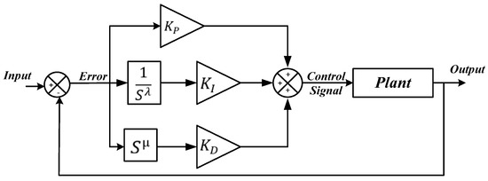
Figure 4. The illustrations of the FOPID Controller.

The standard FOPID controller is called $P{I}^{\lambda }{D}^{\mu }$, where λ and µ can be any real number and stand for integrator and differentiator orders, respectively. The FOPID controller’s transfer function is defined as

$$C\left(s\right)=K_P+K_I\frac{1}{S^{\lambda }}+K_D{S}^{\mathrm{\mu }}$$

(24)

The goal is to derive the optimal values of $K_P$, $K_I$, and $K_D$.

2.4. FOPID Tuning

Despite their advantages, FOPID controllers’ tuning is not straightforward. As such, numerous studies have focused on determining an appropriate tuning technique for FOPID controllers. The existing tuning methods for FOPID controllers are divided into three categories: auto-tuning, robust tuning, and optimal tuning methods [40]. Although these auto-tuning technologies are extremely beneficial in practical applications, they are rarely employed in motion control applications, which require high bandwidths (crossover frequency) [43]. But, for process control (first-order plus delay plants), they are highly useful instruments. Some studies have led to the development of tuning techniques based on H∞ constraints, whereby mathematical techniques like the graphical approach, the Newton–Raphson numerical iterative algorithm, and others are used to meet performance constraints including stability, bandwidth, resilience, and precision [44]. These techniques meet all of the designer’s requirements; however, solving these nonlinear equations is extremely challenging and sometimes impossible. Furthermore, a number of issues arise since several of these methods need the determination of the plant’s dynamic properties. Based on this, it can be stated that the majority of the tuning techniques currently in use are complicated, and each one is limited to a certain class of systems. However, some studies were conducted in an effort to develop a novel tuning technique using optimization techniques such as genetic algorithms and particle swarm optimization [45]. In this method, multiple objective functions and restrictions are addressed when tuning FOPID controllers. These strategies enable controllers to function at their best. This motivates the use of the MFPOA in turning the FOPID controller.

3. Optimization Methodology

3.1. Flower Pollination Algorithm (FPA)

The river pollination method of flowering plants served as the basis for the creation of the FPA (Yang et al. 2012 [46,47]). Through the process of pollination, flowers of a plant are crucial to reproduction. Pollinators including insects, birds, and other animals assist the spread of pollen during pollination. Self-pollination or cross-pollination are terms used to describe pollination. Cross-pollination is the term used to describe the pollination process that occurs when pollen from a plant’s flower is used. Self-pollination, on the other hand, is the act of fertilizing a flower of a plant with pollen from the same flower or from many flowers of the same plant. In the absence of a dependable pollinator, self-pollination frequently takes place. Cross-pollination typically occurs over great distances, and pollinators like bees, bats, birds, and flies are able to travel great distances. Cross-pollination is hence comparable to global pollination. Additionally, a Levy distribution governs how bees and birds fly. Further, the consistency of two blooms can be used as an increment step by comparing or contrasting them. The traditional FPA mostly relies on flower constancy behavior, which is explained in the following manner. Elite flower species can be visited by pollinators, while other flower species can be avoided. Because it facilitates the transmission of pollen to the same plants’ flowers, such flower constancy has the benefit of promoting the reproduction of the same flower species. The following is a list of the FPA’s primary guidelines.

Rule 1: Cross-pollination is a form of global pollination, and pollinators follow the Levy distribution when they fly.

Rule 2: The process of self-pollination is regarded as local pollination.

Rule 3: The likelihood of reproduction is obtained by pollinators like insects and is equivalent to flowering persistence. Based on how similar the two flowers are, this probability is determined.

Rule 4: A switching probability p equal to either 0 or 1 that is slightly skewed in favor of local pollination can be used to control the transition between local and global pollination. The update equations for the FPA are derived by incorporating the aforementioned rules. Mathematically, the first and third principles can be written as Equation (25).

$$u_n^{i+1}=u_n^i+\delta L\left(x\right)\left({u_{best}-u}_n^i\right)$$

(25)

where $L\left(x\right)$ is the Levy-based step size showing the amount of pollination, $\delta$ is a scaling factor to control the step size, and $u_n^i$ represents the n-th pollen or solution $u_n$ at iteration i. $u_{best}$ is the best solution among all the solutions thus far. As a result, L(x) is as in Equation (26).

$$L\approx \frac{x\mathrm{Ґ}\left(\gamma \right)\sin \left(\frac{\pi x}{2}\right)}{\pi }\frac{1}{s^1+x}, s>>s_0>0$$

(26)

where the standard gamma function is represented by $\mathrm{Ґ}\left(\gamma \right)$, and this distribution is acceptable for big steps $s>0$. Despite $s\gg 0$ being necessary, $s_0$ can actually be as low as 0.1. It is challenging to produce pseudorandom step sizes that accurately match the Levy distribution though [48]. As a result, the Mantegna method [49], a useful algorithm that has been documented in the literature, is utilized in the FPA to generate these random values. Two Gaussian distributions, $G_u$ and $G_v$, can be used to derive the step size s in Equation (27).

$$s\frac{G_u}{{\left|G_v\right|}^{\frac{1}{x}}},G_u~N\left(0,{var}^2\right),G_v~N\left(\mathrm{0,1}\right)$$

(27)

The expression $G_u~N\left(0,{var}^2\right)$ denotes that the samples were taken from a Gaussian distribution with a mean and variance of 0 and ${var}^2$, respectively. Equation (28) is used to obtain the variance, or ${var}^2$.

$${var}^2=\left[\frac{\mathrm{Ґ}\left(1+x\right)}{x\mathrm{Ґ}(\left(1+x\right)/2)}.\frac{\sin \pi x/2}{2^{\left(x-1\right)/2}}\right]$$

(28)

The gamma functions $\mathrm{Ґ}\left(1+\lambda \right)=1, \mathrm{Ґ}(\left(1+\lambda \right)/2)=1$ and ${var}^2$ become equal to 1 when the value of x is equal to 1. The update equation for local pollination can be written as Equation (29) based on Rules 2 and 3.

$$u_n^{i+1}=u_n^i+\in \left(u_a^i-u_b^i\right)$$

(29)

The pollen from two separate blooms on the same plant is represented by the letters $u_a^i$ and $u_b^i$. When $\in$ is selected from a uniform distribution in [0, 1], this distribution turns into a local random walk if $u_a^i$ and $u_b^i$ are mathematically taken from the same plant species. Of course, both locally and worldwide influences are involved in the flower pollination process. However, in reality, nearby flowers are more likely to be pollinated by nearby flower pollen than they are by pollen from a great distance away. By allocating a switching probability or proximity probability p as specified in Rule 4, the program can imitate this attribute. It is meritorious to exploit this likelihood to shift from strict local pollination to shared global pollination. It can be started initially by setting the initial value to $\rho =0.5$.

3.2. MFPOA

Adaptive orientation Gaussian (AOG) mutation is employed in the suggested MFPOA approach to optimize the controller settings. The pollen’s characteristics are altered during the pollination process by using the mutation-based flower pollination method. The mutation procedure in the optimization technique often speeds up the solution by changing some of the particle properties. The AOG mutation technique is used in the FPA to accomplish this. The key benefit of the proposed MFPOA is the algorithm’s quicker convergence while maintaining the features of the conventional FPA. The AOG mutation is added to the pollen produced by global pollination in the traditional FPA method following global pollination. As a result, after applying the mutation process [50], Equation (25) is changed into Equation (30):

$$u_{n mut}^{i+1}=u_n^i+\delta L\left(x\right)\left({u_{best}-u}_n^i\right)+\phi \left\{AOG\right\}$$

(30)

where $\phi$ is the probability factor present. Equation (31), which describes the AOG mutation function, is as follows:

$$AOG\left(x\right)=\left(G_{\sigma }\left(x\sin \theta \right)-G_{\sigma }\left(x\cos \theta \right)\right)$$

(31)

$$G_{\sigma }=\frac{1}{\sigma \sqrt{2\pi }}{e}^{\frac{-1}{2}{\left(\frac{x-m}{\sigma }\right)}^2}$$

(32)

where $m$, $\sigma$, $G_{\sigma }\left(x\right),$ and $\theta$ denote the mean, variance, Gaussian function of the variable $x$, and the rotation that must be applied to the function. The mutation is also applied to p. The one from Equation (29) is altered by the mutation process to become Equation (33).

$$u_{n mut}^{i+1}=u_n^i+\in \left(u_a^i-u_b^i\right)+\phi \left\{AOG\right\}$$

(33)

As follows is the probability factor. If the pollen characteristics obtained in the most recent iteration $(i+1)$ using global or local pollination match those obtained in the most recent iteration $\left(i\right)$ using global or local pollination, the probability factor is 1; otherwise, it is zero, and the solution remains the same.

$$\phi =\left\{\begin{array}{c}1 if\left(u_n^{i+1}-u_n^i=0\right)\\ 0 else\end{array}\right.$$

(34)

The AOG-based MFPOA algorithm is provided below in Algorithm 1:

Algorithm 1: AOG-Based MFPOA Algorithm

1. Determine the pollen count using random solutions 2. Determine the ideal response from the starting population 3. Establish a switch probability of p $\mathrm{4.} \mathrm{While} (i < max. No. of generation$) $\mathrm{5.} \mathrm{For} n=1:N$ $\mathrm{6.} \mathrm{If} rand<p$ 7. Create a step vector in d dimensions that follows the Levy distribution 8. Apply Equation (25) to global pollination 9. Use Equation (34) to calculate the mutation probability factor $\mathrm{10.} \mathrm{If} \phi =1$ 11. Apply Equation (29) to determine fresh pollen in global pollination 12. Else 13. Equation (34) is used to calculate new pollen 14. Choose from a uniform distribution in the range [0, 1] 15. Use Equation (33) to carry out local pollination 16. Use Equation (34) to calculate the mutation probability factor $\mathrm{17.} \mathrm{If} \phi =1$ 18. Apply Equation (33) to local pollination to determine fresh pollen 19. Else 20. Equation (29) is used to calculate new pollen 21. End 22. Create fresh approaches 23. If improved solutions emerge, inform the populace of them 24. End 25. Discover the current top option 26. End 27. The fitness solution is the best option

3.3. Implementation of the MFPOA for Optimizing the FOPID Controller

First, a pollen matrix of dimension $3\times n$ is taken into account, with the pollen taken into account as the controller parameters. N is the quantity of plants. In Equation (35), the matrix layout is described:

$$u_n=\left[\begin{array}{cc}\begin{array}{cc}{K}_{P1}& K_{p2}\end{array}& \begin{array}{cc}{K}_{p3}\dots & K_{pn}\end{array}\\ \begin{array}{cc}\begin{array}{c}{{\lambda }_{1}K}_{i1}\\ {\mu }_1{K}_{d1}\end{array}& \begin{array}{c}{{\lambda }_{2}K}_{i2}\\ {\mu }_2{K}_{d2}\end{array}\end{array}& \begin{array}{cc}\begin{array}{c}{{\lambda }_{3}K}_{i3}\dots \\ {\mu }_3{K}_{d3}\dots \end{array}& \begin{array}{c}{{\lambda }_{n}K}_{in}\\ {\mu }_n{K}_{dn}\end{array}\end{array}\end{array}\right]$$

(35)

The best plant with the best fitness function will then be identified utilizing the elements present in each row to calculate the fitness function. The performance criterion shown in Equation (13) will be applied to the controller. Then, update pollen utilizing global pollination or local pollination based on switch probability for the subsequent iteration. The phrase $u_n$ is rendered as $u_{n_m}$ representing the pollen of the plant whose n-th position is at the m-th place. For the proposed application, m for each controller is equal to 4. In local pollination, only the pollen of the same row is taken into account because the pollen of a row comes from the same plant flower. In global pollination, the pollen present in all rows is taken into consideration for pollination. Thus, when the convergence requirement is satisfied, this algorithm yields the best solution set. The Schematics of the MFPOA-based FOPID control is shown in Figure 5.

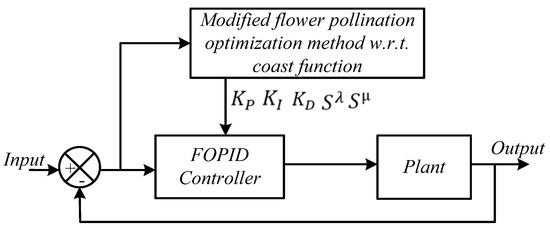
Figure 5. Schematics of the MFPOA-based FOPID control.

3.4. Proposed Cost Function

The fitness function adopted from [51] is as follows:

$$MinJ\left(K_P,K_I,K_D,\lambda ,\mathrm{\mu }\right)=\genfrac{}{}{0pt}{}{Min}{K_P,K_I,K_D,\lambda ,\mathrm{\mu }}\left(e^{-\beta }\left(T_s+T_r\right)+\left(1-e^{-\beta }\right)\left(ITSE+M_P\right)\right)$$

(36)

where $\beta$ is $\mathrm{t}\mathrm{h}\mathrm{e}$ weighting factor, $M_P$ donates overshoot, $T_r$ donates rise time, $T_s$ donates settling time, $Min$ is the minimum of the cost function $J=e^{-\beta }\left(T_s+T_r\right)+\left(1-e^{-\beta }\right)\left(ITSE+M_P\right)$, and $ITSE$ is the integral of the time multiplied square error criterion given by

$$ITSE={\int }_0^{t_{sim}}t{e}^2\left(t\right)dt,$$

(37)

where e(t) is the tracking error, and $t_{sim}$ is the overall simulation time.

$ITSE$ is the most crucial variable in this fitness function. $T_s$, $T_r$, and $M_P$ parameters must all be minimized in order for them to be at their best. In other words, the $T_s$, $T_r$, and $M_P$ parameters are directly and indirectly optimized using this fitness function. The multiple-application Simpson’s 1/3 rule is used to generate the ITSE performance index [52]. Our objective is to use the MFPOA method to determine the best settings for the $P{I}^{\lambda }{D}^{\mu }$ controller.

4. Robust Stability Analysis

The SISO system’s gain is independent of the size of its input. The MIMO system, however, offers more degrees of freedom. Because of this, the gain is influenced by the direction of the disturbance d, as detailed in [52]. It is crucial to perform a robust stability study of MIMO systems due to model uncertainty and other parameter changes. The stability analysis is assessed using the singular-value uncertainty model. The schematic of the input uncertainty taken into consideration throughout the analysis is shown in Figure 6a. The following conditions must be met for the closed-loop system to be stable.

$$‖{∆}_I\left(j\omega \right)‖<\frac{1}{\overline{{\vartheta }_1}}$$

(38)

where $M\left(s\right)[1+{∆}_I\left(s\right)]$ is the input uncertainty, and $\overline{{\vartheta }_1}$ is the maximum singular value (MSV) of the closed-loop system $C\left(s\right)M\left(s\right)/(1+C\left(s\right)M\left(s\right))$. The MSV of $N$ can be calculated using the maximum gain. Moreover, the matrix can be reduced to its single value as

$$M=⊑{\varrho \updownarrow }^{*}$$

(39)

where $\varrho$ is a matrix of the order x × y, and $\updownarrow$ and $⊑$ are unitary matrices of the order $y\times y$ and $x\times x$, respectively. Similar to the discussion in [53], the closed-loop system for the multiplicative output uncertainty $M\left(s\right)[1+{∆}_o\left(s\right)]$ will be stable if the following requirements are met:

$$‖{∆}_o\left(j\omega \right)‖<\frac{1}{\overline{{\vartheta }_2}}$$

(40)

where $\overline{{\vartheta }_2}$ is the MSV of the closed-loop system $C\left(s\right)M\left(s\right)/(1+C\left(s\right)M\left(s\right))$.

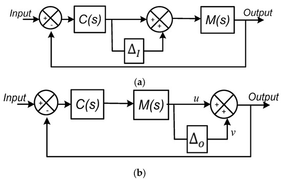
Figure 6. Illustrations for input uncertainty in (a) output uncertainty (b).

Examining the frequency graphs of Equations (38) and (40) will reveal the stability bounds of the closed-loop system. The stability of the system can be determined by looking at the area under the curve. As a result, it is simple to examine the controllers’ stability. The controller that covers the biggest area beneath the curve will be the most stable one.

5. Simulation Results and Discussion

Simulated analysis of the proposed control scheme was carried out in the Matlab/Simulink environment. Three separate case studies were taken into account to demonstrate the effectiveness of the control method. Comparing the performance and robustness to the techniques outlined in the aforementioned literature allowed for evaluation.

5.1. Case 1 (2 × 2) VL Column System

The benchmark VL column example provided by Luyben (1986) is a TITO process with greater input and output interaction [54]. The VL column transfer function structure is provided below.

$$M\left(s\right)=\left[\begin{array}{cc}\frac{-2.2e^{-s}}{7s+1}& \frac{1.3e^{-0.3s}}{7s+1}\\ \frac{2.8e^{-1.8s}}{9.5s+1}& \frac{4.3e^{-0.35s}}{9.2s+1}\end{array}\right]$$

(41)

The ultimate control assumption, which forms the basis of the EOTF/ETF models, can only be verified by including a decoupler in the open-loop model. Decouplers can be created using Equation (3) as

$$D\left(s\right)=\left[\begin{array}{cc}1& 0.5909\\ \frac{(5.9907s+0.6512)e^{-1.45s}}{9.5s+1}& e^{-0.7s}\end{array}\right]$$

(42)

The decoupler D(s) includes an additional time delay,

$$G\left(s\right)D\left(s\right)=\left[\begin{array}{cc}{g}_{11}\left(s\right)& g_{12}\left(s\right)\\ g_{21}\left(s\right)& g_{22}\left(s\right)\end{array}\right]\left[\begin{array}{cc}1& d_{12}\left(s\right)e^{0.7s}\\ d_{21}\left(s\right)& e^{-0.7s}\end{array}\right]=\left[\begin{array}{cc}{g}_{11}^{*}\left(s\right)& 0\\ 0& g_{22}^{*}\left(s\right)\end{array}\right]$$

(43)

The decoupled processes are

$$g_{11}^{*}\left(s\right)=\frac{-1.3535e^{-0.9559s}}{6.691s+1}$$

(44)

$$g_{22}^{*}\left(s\right)=\frac{2.6455e^{-1.034s}}{8.794s+1}$$

(45)

Additionally, the described optimization issue in Equation (36) is where the decentralized FOPI controller is derived.

$$C\left(s\right)=\left[\begin{array}{cc}-2.5858-\frac{0.3865}{s}& 0\\ 0& 1.6066+\frac{0.1941}{s}\end{array}\right]$$

(46)

The MFPOA method was implemented in MATLAB. The parameters utilized in this paper’s MFPOA-based simulations are shown in Table 1.

Table 1. Parameter settings for the simulation.

Parameter	Value
Population size (n)	50
Probability of switching (p)	0.8
Number of iterations	100
Number of variables	5
$\mathrm{Maximum} \mathrm{limits} [K_P, K_I, K_D, \lambda , \mu$]	40, 20, 20, 1, 1
Minimum limits [$K_P, K_I, K_D, \lambda , \mu$]	0, 0, 0, 0, 0
$\beta$	2.5

Figure 7 displays the closed-loop response for the VL column. Both references apply the unit step changes. The setpoint of loop 2 is altered from 0.2 to 1 at t = 100, as shown in Figure 8. A traditional PID controller and a proposed controller are contrasted. It is evident from the figure that the proposed FOPID controller outperforms the PID controller in terms of performance. The proposed FOPID controller’s quicker regulatory reaction significantly minimized the interaction effect.

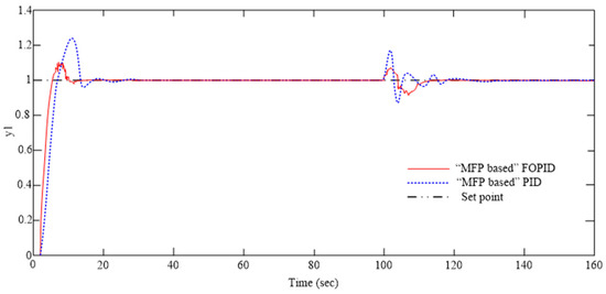
Figure 7. Servo and regulatory response for the VL column (Equation (44)).

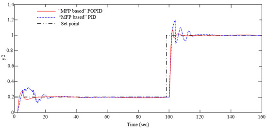
Figure 8. Servo and regulatory response for the VL column (Equation (45)).

The setting of the optimized PID and FOPID are found through minimization of the cost function for the ETF model ($g_{11}^{*}\left(s\right), g_{22}^{*}\left(s\right)$) using the MFPOA. The optimal controller variables are presented in Table 2. The comparisons of the performance indexes are also presented in the same table. The minimum values of $M_P$, $T_r$, and $T_s$ are recorded by the proposed FOPID controller based on the MFPOA. Thus, it can be observed that the proposed FOPID controller based on the MFPOA may reduce error and achieve the design objectives.

Table 2. Optimal values and performance indexes of the MFPOA-based controller and MFPOA-based PID controller for the ETF model ($g_{11}^{*}\left(s\right), g_{22}^{*}\left(s\right)$).

Loop	Controller	${\mathit{K}}_{\mathit{P}}$	${\mathit{K}}_{\mathit{I}}$	${\mathit{K}}_{\mathit{D}}$	$\mathit{\lambda }$	$\mathit{\mu }$	${\mathit{M}}_{\mathit{P}}$	${\mathit{T}}_{\mathit{r}}$	${\mathit{T}}_{\mathit{s}}$
$g_{11}^{*}\left(s\right)$	MFPOA-based FOPID	36.81	5.69	16.62	1	0.0281	0	0.0399	0.0756
	MFPOA-based PID	38.67	3.48	10.12	-	-	0	0.087	0.25
$g_{22}^{*}\left(s\right)$	MFPOA-based FOPID	37.92	17.60	19.51	0.212	0.167	0	0.0020	0.0068
	MFPOA-based PID	36.34	37.31	0.62	-	-	1.1632	0.0053	0.0081

Stability Analysis

Figure 9 and Figure 10 present the controller stability analysis. The sensitivity function’s singular values are used to validate the analysis. Figure 9 and Figure 10 show the closed-loop system’s stability regions as given by Equations (39) and (40). The stable region is the area that the curve encloses. The figures indicate that the suggested MFPOA-based FOPID controller has more stable zones. Additionally, the peak value is below 1.5, meaning it is desirable.

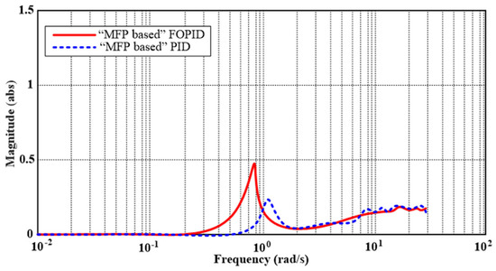
Figure 9. Singular values of the sensitivity function: Equation (44).

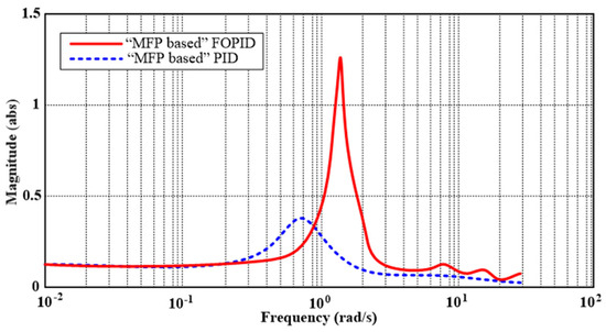
Figure 10. Singular values of the sensitivity function: Equation (45).

5.2. Case 2 (3 × 3) Shell Heavy Oil Fractionator

According to Prett et al. [54] and Lawal and Zhang [55], the Shell heavy oil fractionator (SHOF) is a multivariable process involving loop interactions and temporal delays. This kind of distillation column separates the crude oil from the mixture by making use of the variations in boiling points. The MIMO transfer function of the process is

$$M\left(s\right)=\left[\begin{array}{ccc}\frac{4.05e^{-27s}}{50s+1}& \frac{1.775e^{-28s}}{60s+1}& \frac{5.88e^{-27s}}{50s+1}\\ \frac{5.39e^{-18s}}{50s+1}& \frac{5.72e^{-14s}}{60s+1}& \frac{6.90e^{-15s}}{40s+1}\\ \frac{4.38e^{-20s}}{33s+1}& \frac{4.42e^{-22s}}{44s+1}& \frac{7.20}{19s+1}\end{array}\right]$$

(47)

Decouplers can be created using Equation (3) as

$$D\left(s\right)=\left[\begin{array}{ccc}1& \frac{(-88.5s+1.77)e^{-s}}{243s+4.05}& -1.45\\ \frac{(-323.4s+5.39)e^{-4s}}{286s+5.72}& 1& \frac{(-345s+6.90)e^{-s}}{215.6s+5.39}\\ \frac{(-83.2s+4.38)e^{-20s}}{237.6s+7.2}& \frac{(-83.98s+4.42)e^{-22s}}{316.8s+7.2}& 1\end{array}\right]$$

(48)

The FOPDT models are generated from Equations (9) through (11) and are presented as such in [29].

$$g_{11}^{*}\left(s\right)=\frac{-1.19e^{-16.75s}}{1.95s+1}$$

(49)

$$g_{22}^{*}\left(s\right)=\frac{-0.875e^{-11.57s}}{1.86s+1}$$

(50)

$$g_{33}^{*}\left(s\right)=\frac{-4.8e^{-0.007s}}{25.26s+1}$$

(51)

Moreover, Equation (36) defines the optimization problem from which the decentralized FOPI controller is derived.

$$C\left(s\right)=\left[\begin{array}{ccc}10.5+\frac{1.8}{s}& 0& 0\\ 0& 13.8+\frac{3.9}{s}& 0\\ 0& 0& 9.1+\frac{4.2}{s}\end{array}\right]$$

(52)

As seen from Figure 11, Figure 12 and Figure 13, the primary goal is to control the flow rate on top-draw, side-draw, and bottom reflux duty, respectively, in order to keep the top-end-point composition (y1), side-end-point composition (y2), and bottom reflux temperature (y3) at acceptable values. The proposed controller is compared with a conventional PID controller. According to the proposed coast function, less overshoot, rise time, and settling time are required to meet the design criteria. In addition, input and output disturbances are used to validate the disturbance rejection. A step signal in the form of a disturbance is injected into the process input (at 100 s) and output (at 140 s). Figure 11, Figure 12 and Figure 13 show the reference tracking and their corresponding controller outputs. The design specifications are met. The optimal controller variables are presented in Table 3. Additionally, the comparisons of the performance indexes are presented in the same table. The proposed MFPOA-based FOPID controller records the minimum values of $M_P$, $T_r$, and $T_s$. Therefore, it can be concluded that the proposed MFPOA-based FOPID controller can decrease error and meet the design goals.

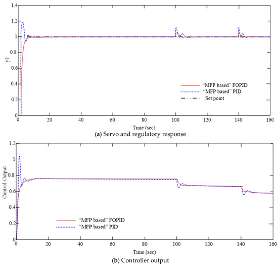
Figure 11. Response of Equation (49).

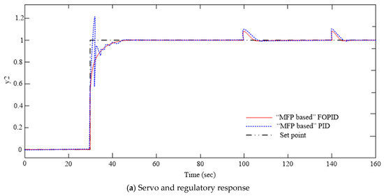
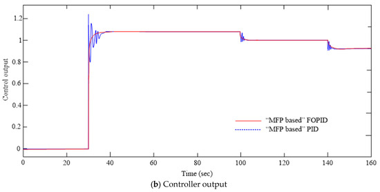
Figure 12. Response of Equation (50).

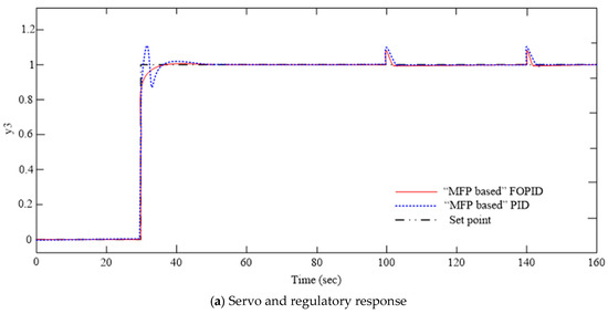
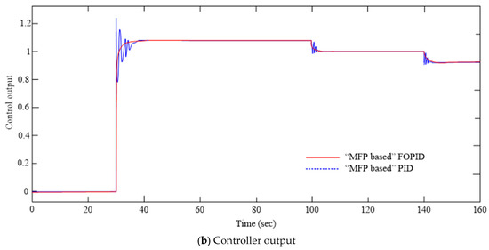
Figure 13. Response of Equation (51).

Table 3. Optimal values and performance indexes of the MFPOA-based controller and MFPOA-based PID controller for the Shell heavy oil fractionator model ($g_{11}^{*}\left(s\right), g_{22}^{*}\left(s\right), g_{33}^{*}\left(s\right)$).

Loop	Controller	${\mathit{K}}_{\mathit{P}}$	${\mathit{K}}_{\mathit{I}}$	${\mathit{K}}_{\mathit{D}}$	$\mathit{\lambda }$	$\mathit{\mu }$	${\mathit{M}}_{\mathit{P}}$	${\mathit{T}}_{\mathit{r}}$	${\mathit{T}}_{\mathit{s}}$
$g_{11}^{*}$	MFPOA-based FOPID	32.76	5.06	15.96	1	0.032	0	0.0048	0.0839
	MFPOA-based PID	34.42	3.10	9.72	-	-	0	0.0104	0.2775
$g_{22}^{*}\left(s\right)$	MFPOA-based FOPID	34.90	11.08	16.81	0.89	0.113	0	0.0025	0.0457
	MFPOA-based PID	31.03	18.97	5.16	-	-	0.9604	0.0055	0.1433
$g_{33}^{*}\left(s\right)$	MFPOA-based FOPID	33.75	15.66	18.73	0.25	0.192	0	0.0002	0.0075
	MFPOA-based PID	32.34	33.21	0.60	-	-	1.1399	0.0006	0.0090

Stability Analysis

Figure 14, Figure 15 and Figure 16 present the controller stability analysis. The sensitivity function’s singular values are used to validate the analysis. Figure 14, Figure 15 and Figure 16 depict the closed-loop system’s stability regions as given by Equations (39) and (40). The stable region is the area that the curve encloses. The figures suggest that the suggested MFPOA-based FOPID controller has more stable zones. Additionally, the peak value is below 1.5, meaning it is desirable.

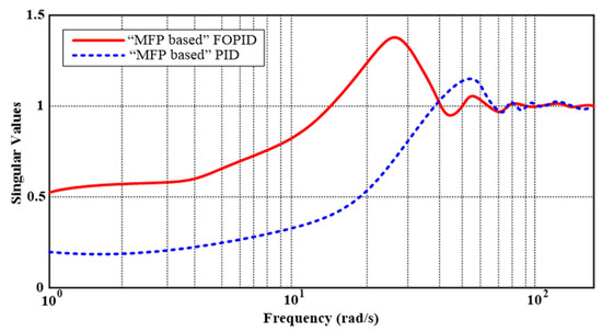
Figure 14. Singular values of the sensitivity function: Equation (49).

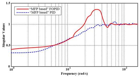
Figure 15. Singular values of the sensitivity function: Equation (50).

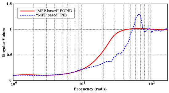
Figure 16. Singular values of the sensitivity function: Equation (51).

6. Conclusions

This study provides a decentralized control strategy for higher-order systems based on the MFPOA. The objective is to optimize the control performance, stability, and robustness in complex and interconnected systems by putting constraints on the maximum overshoot ($M_p$), rising time ($T_r$), and settling time ($T_s$). Effective parameter optimization is made possible by the MFPOA integration, which satisfies the requirements set forth for each subsystem in the decentralized control architecture. Compared to the traditional PID control method, the decentralized control strategy using the MFPOA-based FOPID controller achieves greater control performance, fewer interactions across subsystems, and enhanced stability margins.

The results demonstrate how successful the suggested control strategy is. The suggested approach offers a dependable and effective way to create high-performance and durable FOPID controllers that meet the unique needs of intricately linked systems. Extensive simulation research on two distinct systems confirmed the efficacy of the suggested methodology. While the robustness was confirmed using noise signals and parameter changes, the disturbance rejection was examined with input and output disturbances.

The comparisons of the MFPOA and classical FPA as well as other commonly used algorithms, such as GA, PSO should be considered in future research. In addition, the application of the proposed controller on higher-order systems (like $4\times 4, 5\times 5,$ etc.) should be considered.

References

- Borase, R.P.; Maghade, D.K.; Sondkar, S.Y.; Pawar, S.N. A review of PID control, tuning methods and applications. Int. J. Dyn. Control 2021, 9, 818–827. [Google Scholar] [CrossRef]
- Shah, P.; Agashe, S. Review of fractional PID controller. Mechatronics 2016, 38, 29–41. [Google Scholar] [CrossRef]
- Jamil, A.A.; Tu, W.F.; Ali, S.W.; Terriche, Y.; Guerrero, J.M. Fractional-order PID controllers for temperature control: A review. Energies 2022, 15, 3800. [Google Scholar] [CrossRef]
- Bingi, K.; Ibrahim, R.; Karsiti, M.N.; Hassan, S.M.; Harindran, V.R. Fractional-Order Systems and PID Controllers; Springer International Publishing: Cham, Switzerland, 2020; Volume 264. [Google Scholar]
- Xie, Y.; Tang, X.; Song, B.; Zhou, X.; Guo, Y. Model-free tuning strategy of fractional-order pi controller for speed regulation of permanent magnet synchronous motor. Trans. Inst. Meas. Control 2019, 41, 23–35. [Google Scholar] [CrossRef]
- Stanisławski, R.; Rydel, M.; Li, Z. A new reduced-order implementation of discrete-time fractional-order pid controller. IEEE Access 2022, 10, 17417–17429. [Google Scholar] [CrossRef]
- Al-Saggaf, U.M.; Mehedi, I.M.; Mansouri, R.; Bettayeb, M. Rotary flexible joint control by fractional order controllers. Int. J. Control Autom. Syst. 2017, 15, 2561–2569. [Google Scholar] [CrossRef]
- Dwivedi, P.; Pandey, S.; Junghare, A. Performance analysis and experimental validation of 2-dof fractional-order controller for underactuated rotary inverted pendulum. Arab. J. Sci. Eng. 2017, 42, 5121–5145. [Google Scholar] [CrossRef]
- Tepljakov, A.; Alagoz, B.B.; Yeroglu, C.; Gonzalez, E.A.; Hosseinnia, S.H.; Petlenkov, E.; Ates, A.; Cech, M. Towards industrialization of fopid controllers: A survey on milestones of fractional order control and pathways for future developments. IEEE Access 2021, 9, 21016–21042. [Google Scholar] [CrossRef]
- Hou, Z.; Xiong, S. On model-free adaptive control and its stability analysis. IEEE Trans. Autom. Control 2019, 64, 4555–4569. [Google Scholar] [CrossRef]
- Huang, L.; Deng, L.; Li, A.; Gao, R.; Zhang, L.; Lei, W. A novel approach for solar greenhouse air temperature and heating load prediction based on laplace transform. J. Build. Eng. 2021, 44, 102682. [Google Scholar] [CrossRef]
- Ardjal, A.; Bettayeb, M.; Mansouri, R.; Zouak, B. Design and implementation of a model-free fractional order intelligent PI fractional order sliding mode controller for water level tank system. ISA Trans. 2022, 127, 501–510. [Google Scholar] [CrossRef]
- Yakoub, Z.; Amairi, M.; Chetoui, M.; Saidi, B.; Aoun, M. Model-free adaptive fractional order control of stable linear timevarying systems. ISA Trans. 2017, 67, 193–207. [Google Scholar] [CrossRef] [PubMed]
- Ibraheem, G.A.R.; Azar, A.T.; Ibraheem, I.K.; Humaidi, A.J. A novel design of a neural network-based fractional pid controller for mobile robots using hybridized fruit fly and particle swarm optimization. Complexity 2020, 2020, 1–18. [Google Scholar] [CrossRef]
- Norsahperi, N.; Danapalasingam, K. Particle swarm-based and neuro-based fopid controllers for a twin rotor system with improved tracking performance and energy reduction. ISA Trans. 2020, 102, 230–244. [Google Scholar] [CrossRef] [PubMed]
- Kumar, R.; Sinha, N. Voltage stability of solar dish-stirling based autonomous dc microgrid using grey wolf optimised fopidcontroller. Int. J. Sustain. Energy 2021, 40, 412–429. [Google Scholar] [CrossRef]
- Rais, M.C.; Dekhandji, F.Z.; Recioui, A.; Rechid, M.S.; Djedi, L. Comparative study of optimization techniques based pid tuning for automatic voltage regulator system. Eng. Proc. 2022, 14, 21. [Google Scholar]
- Mughees, A.; Mohsin, S.A. Design and control of magnetic levitation system by optimizing fractional order pid controller using ant colony optimization algorithm. IEEE Access 2020, 8, 116704–116723. [Google Scholar] [CrossRef]
- Łapa, K. Elastic FOPID+ FIR Controller Design Using Hybrid Population-Based Algorithm. In Information Systems Architecture and Technology: Proceedings of 37th International Conference on Information Systems Architecture and Technology–ISAT 2016–Part II; Springer International Publishing: Cham, Switzerland, 2017; pp. 15–26. [Google Scholar]
- Moafi, M.; Marzband, M.; Savaghebi, M.; Guerrero, J.M. Energy management system based on fuzzy fractional order PID controller for transient stability improvement in microgrids with energy storage. Int. Trans. Electr. Energy Syst. 2016, 26, 2087–2106. [Google Scholar] [CrossRef]
- Zamani, M.; Karimi-Ghartemani, M.; Sadati, N.; Parniani, M. Design of a fractional order PID controller for an AVR using particle swarm optimization. Control Eng. Pract. 2009, 17, 1380–1387. [Google Scholar] [CrossRef]
- Zhang, Y.; Li, J. Fractional-order PID controller tuning based on genetic algorithm. In Proceedings of the 2011 International Conference on Business Management and Electronic Information, Guangzhou, China, 13–15 May 2011; Volume 3, pp. 764–767. [Google Scholar]
- Lazim, D.; Zain, A.M.; Bahari, M.; Omar, A.H. Review of modified and hybrid flower pollination algorithms for solving optimization problems. Artif. Intell. Rev. 2019, 52, 1547–1577. [Google Scholar] [CrossRef]
- Nabil, E. A modified flower pollination algorithm for global optimization. Expert. Syst. Appl. 2016, 57, 192–203. [Google Scholar] [CrossRef]
- Abdel-Basset, M.; Mohamed, R.; Saber, S.; Askar, S.S.; Abouhawwash, M. Modified flower pollination algorithm for global optimization. Mathematics 2021, 9, 1661. [Google Scholar] [CrossRef]
- Rajeswari, C.; Santhi, M. Modified flower pollination algorithm for optimizing FOPID controller and its application with the programmable n-level inverter using fuzzy logic. Soft Comput. 2021, 25, 2615–2633. [Google Scholar] [CrossRef]
- Govind, K.A.; Mahapatra, S.; Mahapatro, S.R. A Comparative Analysis of Various Decoupling Techniques Using Frequency Domain Specifications. In Proceedings of the 2023 3rd International Conference on Artificial Intelligence and Signal Processing (AISP), Vijayawada, India, 18–20 March 2023; pp. 1–6. [Google Scholar]
- Rajapandiyan, C.; Chidambaram, M. Controller design for MIMO processes based on simple decoupled equivalent transfer functions and simplified decoupler. Ind. Eng. Chem. Res. 2012, 51, 12398–12410. [Google Scholar] [CrossRef]
- Wang, Q.G.; Ye, Z.; Cai, W.J.; Hang, C.C. PID Control for Multivariable Processes; Springer: Berlin/Heidelberg, Germany, 2008. [Google Scholar]
- Abdeljawad, T. On Riemann and Caputo fractional differences. Comput. Math. Appl. 2011, 62, 1602–1611. [Google Scholar] [CrossRef]
- Li, C.; Qian, D.; Chen, Y. On Riemann-Liouville and caputo derivatives. Discret. Dyn. Nat. Soc. 2011, 2011, 562494. [Google Scholar] [CrossRef]
- Jiang, Y.; Zhang, B. Comparative study of Riemann–Liouville and Caputo derivative definitions in time-domain analysis of fractional-order capacitor. IEEE Trans. Circuits Syst. II Express Briefs 2019, 67, 2184–2188. [Google Scholar] [CrossRef]
- Garrappa, R. A Grunwald–Letnikov scheme for fractional operators of Havriliak–Negami type. Math. Comput. Sci. Eng. Ser. 2014, 34, 70–76. [Google Scholar]
- Bingul, Z.; Karahan, O. Comparison of PID and FOPID controllers tuned by PSO and ABC algorithms for unstable and integrating systems with time delay. Optim. Control Appl. Methods 2018, 39, 1431–1450. [Google Scholar] [CrossRef]
- Baranowski, J.; Bauer, W.; Zagórowska, M.; Dziwiński, T.; Piątek, P. Time-domain oustaloup approximation. In Proceedings of the 2015 20th International Conference on Methods and Models in Automation and Robotics (MMAR), Miedzyzdroje, Poland, 24–27 August 2015; pp. 116–120. [Google Scholar]
- Oprzędkiewicz, K.; Mitkowski, W.; Gawin, E. An estimation of accuracy of Oustaloup approximation. In Challenges in Automation, Robotics and Measurement Techniques; Springer International Publishing: Cham, Switzerland, 2016; pp. 299–307. [Google Scholar]
- Gao, Z.; Liao, X. Improved Oustaloup approximation of fractional-order operators using adaptive chaotic particle swarm optimization. J. Syst. Eng. Electron. 2012, 23, 145–153. [Google Scholar] [CrossRef]
- Matignon, D. Stability results for fractional differential equations with applications to control processing. In Proceedings of the Symposium on Modelling, Analysis and Simulation: CESA’96 IMACS Multiconference, Computational Engineering in Systems Applications, Lille, France, 9–12 July 1996; Volume 2, No. 1. pp. 963–968. [Google Scholar]
- Zhang, Y.; Lin, P.; Sun, W. Nonlinear control and circuit implementation in coupled nonidentical fractional-order chaotic systems. Fractal Fract. 2022, 6, 428. [Google Scholar] [CrossRef]
- Dastjerdi, A.A.; Saikumar, N.; HosseinNia, S.H. Tuning guidelines for fractional order PID controllers: Rules of thumb. Mechatronics 2018, 56, 26–36. [Google Scholar] [CrossRef]
- Muresan, C.I.; Birs, I.; Ionescu, C.; Dulf, E.H.; De Keyser, R. A review of recent developments in autotuning methods for fractional-order controllers. Fractal Fract. 2022, 6, 37. [Google Scholar] [CrossRef]
- Li, B.; Zhao, X.; Liu, Y.; Zhao, X. Robust H∞ control of fractional-order switched systems with order 0 < α< 1 and uncertainty. Fractal Fract. 2022, 6, 164. [Google Scholar]
- Nassef, A.M.; Abdelkareem, M.A.; Maghrabie, H.M.; Baroutaji, A. Metaheuristic-Based Algorithms for Optimizing Fractional-Order Controllers—A Recent, Systematic, and Comprehensive Review. Fractal Fract. 2023, 7, 553. [Google Scholar] [CrossRef]
- Yang, X.S. Flower pollination algorithm for global optimization. In Proceedings of the International Conference on Unconventional Computing and Natural Computation, Orléans, France, 3–7 September 2012; Springer: Berlin/Heidelberg, Germany, 2012; pp. 240–249. [Google Scholar]
- Yang, X.S.; Karamanoglu, M.; He, X. Flower pollination algorithm: A novel approach for multiobjective optimization. Eng. Optim. 2014, 46, 1222–1237. [Google Scholar] [CrossRef]
- Pavlyukevich, I. Lévy flights, non-local search and simulated annealing. J. Comput. Phys. 2007, 226, 1830–1844. [Google Scholar] [CrossRef]
- Mantegna, R.N. Fast, accurate algorithm for numerical simulation of Levy stable stochastic processes. Phys. Rev. E 1994, 49, 4677. [Google Scholar] [CrossRef]
- Hamza, M.F. Modified Flower Pollination Optimization Based Design of Interval Type-2 Fuzzy PID Controller for Rotary Inverted Pendulum System. Axioms 2023, 12, 586. [Google Scholar] [CrossRef]
- Nasirpour, N.; Balochian, S. Optimal design of fractional-order PID controllers for multi-input multi-output (variable air volume) air-conditioning system using particle swarm optimization. Intell. Build. Int. 2017, 9, 107–119. [Google Scholar] [CrossRef]
- Hoffman, J.D.; Frankel, S. Numerical Methods for Engineers and Scientists; CRC Press: Boca Raton, FL, USA, 2018. [Google Scholar]
- Besta, C.S.; Chidambaram, M. Tuning of multivariable PI controllers by BLT method for TITO systems. Chem. Eng. Commun. 2016, 203, 527–538. [Google Scholar] [CrossRef]
- Vu TN, L.; Lee, M. Multi-loop PI controller design based on the direct synthesis for interacting multi-time delay processes. ISA Trans. 2010, 49, 79–86. [Google Scholar]
- Lakshmanaprabu, S.K.; Elhoseny, M.; Shankar, K. Optimal tuning of decentralized fractional order PID controllers for TITO process using equivalent transfer function. Cogn. Syst. Res. 2019, 58, 292–303. [Google Scholar] [CrossRef]
- Prett, D.M.; García, C.E.; Ramaker, B.L. The Second Shell Process Control Workshop: Solutions to the Shell Standard Control Problem; Elsevier: Amsterdam, The Netherlands, 2017. [Google Scholar]
- Lawal, S.A.; Zhang, J. Actuator fault monitoring and fault tolerant control in distillation columns. Int. J. Autom. Comput. 2017, 14, 80–92. [Google Scholar] [CrossRef]
Disclaimer/Publisher’s Note: The statements, opinions and data contained in all publications are solely those of the individual author(s) and contributor(s) and not of MDPI and/or the editor(s). MDPI and/or the editor(s) disclaim responsibility for any injury to people or property resulting from any ideas, methods, instructions or products referred to in the content. |
© 2024 by the author. Licensee MDPI, Basel, Switzerland. This article is an open access article distributed under the terms and conditions of the Creative Commons Attribution (CC BY) license (https://creativecommons.org/licenses/by/4.0/).