Issues on a 2–Dimensional Quadratic Sub–Problem and Its Applications in Nonlinear Programming: Trust–Region Methods (TRMs) and Linesearch Based Methods (LBMs)

Abstract

This paper analyses the solution of a specific quadratic sub-problem, along with its possible applications, within both constrained and unconstrained Nonlinear Programming frameworks. We give evidence that this sub–problem may appear in a number of Linesearch Based Methods (LBM) schemes, and to some extent it reveals a close analogy with the solution of trust–region sub–problems. Namely, we refer to a two-dimensional structured quadratic problem, where five linear inequality constraints are included. Finally, we detail how to compute an exact global solution of our two-dimensional quadratic sub-problem, exploiting first order Karush-Khun-Tucker (KKT) conditions.

1. Introduction

There are plenty of real problems where the minimization of a twice continuously differentiable functional $f:{\mathbb{R}}^n\to \mathbb{R}$ is sought, (possibly) subject to several linear and nonlinear constraints. Among authoritative textbooks, where such problems are widely detailed, we can surely find [1,2,3]. Such general problems typically require the solution to a sequence of simple sub-problems with the following pattern:

$$\begin{array}{c}{\displaystyle \underset{x}{min}{\phi }_k\left(x\right)}\hfill \\ \mathrm{s}.\mathrm{t}.x\in D_k,\hfill \end{array}{D}_k:\left\{\begin{array}{c}{A}_{k}x+u_k=0\hfill \\ B_{k}x+v_k\le 0,\hfill \end{array}\right.$$

(1)

where $A_k\in {\mathbb{R}}^{m_k\times n}$, $B_k\in {\mathbb{R}}^{p_k\times n}$, $u_k\in {\mathbb{R}}^{m_k}$, $v_k\in {\mathbb{R}}^{p_k}$, $m_k,p_k\ge 1$ and $k\ge 1$. Furthermore, ${\phi }_k\left(x\right)$ represents a model of the smooth function $f\left(x\right)$ at the current iterate $x_k$ and the feasible set $D_k$ represents a linearization of the constraints.

As is well known, affine and quadratic polynomials based on Taylor’s expansion are often adopted to represent the models $\left\{{\phi }_k\left(x\right)\right\}$, but valid alternatives also include least squares approximations, Radial Basis Functions, metamodels based on Splines, B-Splines, Kriging, etc. [4,5]. We remark that the advantage of solving the sequence of sub-problems (1) in place of the original nonlinearly constrained problem, within a suitable convergence framework, essentially relies on their simplicity. In particular, in this paper our focus is on investigating the role and the properties of the next problem (2), that represents a special sub-case of the more general problem (1). More specifically, we consider the case where in (1) the feasible set $D_k$ includes only a finite number of inequalities, and the function ${\phi }_k\left(x\right)$ is a quadratic functional, i.e., we focus on the sub-problem and drop the dependency on k

$$\begin{array}{c}{\displaystyle \underset{\alpha ,\beta }{min}\phi \left(x\right)=\frac{1}{2}{x}^{T}Qx+b^{T}x+c}\hfill \\ x=\overline{x}+\alpha d+\beta z\hfill \\ a_1\le \alpha \le b_1\hfill \\ a_2\le \beta \le b_2\hfill \\ {ϵ}_1\alpha +{ϵ}_2\beta \le {ϵ}_3\hfill \end{array}$$

(2)

where $Q\in {\mathbb{R}}^{n\times n}$, $b,\overline{x}\in {\mathbb{R}}^n$, $c\in \mathbb{R}$, $d,z\in {\mathbb{R}}^n$ are given n-real search directions, and $a_1\le b_1$, $a_2\le b_2$. Despite the apparent specific structure of (2), a number of real applications may benefit from its solution, as partly described in Section 4 (see also [6] for a general perspective and [7] for a more recent similar viewpoint within neural network frameworks).

As an example of versatility for the structure of (2), both in TRMs and LBMs, we will shortly consider how it may be possibly successfully embedded within the framework of Truncated Newton’s methods (TNMs—see Table 1).

Table 1. A standard framework for linesearch-based TNMs for large-scale problems. The alternative of possibly using negative curvature directions allows for convergence to stationary limit points which fulfill second-order necessary optimality conditions.

Set $x_0\in {\mathbb{R}}^n$

Set ${\eta }_k\in [0,1)$ for any k, with $\left\{{\eta }_k\right\}\to 0$

OUTER ITERATIONS

for  $k=0,1,\dots$

Compute $b\approx \nabla f\left(x_k\right)$ and $Q\approx {\nabla }^{2}f\left(x_k\right)$; if $\parallel b\parallel$ is small then STOP

INNER ITERATIONS

-   Compute $d_k$, which approximately solves Newton’s equation

$Qd+b=0$, i.e., it satisfies the truncation rule $\parallel Q{d}_k+b\parallel \le {\eta }_k\parallel b\parallel$

-   Possibly compute a bounded negative curvature direction $z_k$ at $x_k$

Use a criterion to either combine $d_k$ and $z_k$, or choose between $d_k$ and $z_k$

If the directions $d_k$ and $z_k$ were combined, set $v_k\left(\alpha \right)={\omega }_1\left(\alpha \right)d_k+{\omega }_2\left(\alpha \right)z_k$, and

use a curvilinear linesearch procedure to select $\alpha \leftarrow {\alpha }_k$. Otherwise, set $v_k\left(\alpha \right)=\alpha \overline{d}$

with $\overline{d}\in \{d_k,z_k\}$, and use an Armijo-type procedure to select $\alpha \leftarrow {\alpha }_k$

Update $x_{k+1}=x_k+v_k\left({\alpha }_k\right)$

endfor

Where (see also [8,9,10,11,12,13,14])

• $d\in {\mathbb{R}}^n$ represents an approximate Newton-type direction, at the current feasible point $\overline{x}\in {\mathbb{R}}^n$;
• $z\in {\mathbb{R}}^n$ represents a negative curvature direction for the nonlinear function $f\left(x\right)$, at the current feasible point $\overline{x}\in {\mathbb{R}}^n$;
• $Q\in {\mathbb{R}}^{n\times n}$ represents the exact/approximate Hessian matrix of $f\left(x\right)$ at $\overline{x}$;
• $b\in {\mathbb{R}}^n$ represents the exact/approximate Gradient vector of $f\left(x\right)$ at $\overline{x}$;
• $\alpha$ and $\beta$ are steplengths along the directions $d,z\in {\mathbb{R}}^n$ (i.e., following the taxonomy of Table 1, we have $\alpha \leftarrow {\omega }_1\left(\alpha \right)$ and $\beta \leftarrow {\omega }_2\left(\alpha \right)$), with $-\infty <a_1\le b_1<+\infty$ and $-\infty <a_2\le b_2<+\infty$. The constraint ${\epsilon }_1\alpha +{\epsilon }_2\beta \le {\epsilon }_3$ potentially plays a multi-purpose role, modeling for instance the gradient-related property for the search direction $\alpha d+\beta z\in {\mathbb{R}}^n$ at $\overline{x}$, i.e.,

$${(\alpha d+\beta z)}^T\nabla f\left(\overline{x}\right)\le -\overline{c}{\parallel \nabla f\left(\overline{x}\right)\parallel }^h,$$

(3)

being

$$\left\{\begin{array}{c}{\epsilon }_1=d^T\nabla f\left(\overline{x}\right),\hfill \\ \hfill \\ {\epsilon }_2=z^T\nabla f\left(\overline{x}\right),\hfill \\ \hfill \\ {\epsilon }_3=-\overline{c}{\parallel \nabla f\left(\overline{x}\right)\parallel }^h,\overline{c},h>0.\hfill \end{array}\right.$$

The availability of an (exact) global solution for (2) may also suggest some alternatives to Table 1, either selecting a TRM or a LBM framework, or combining the two approaches. In particular, the scheme in Table 2 represents an immediate acceleration scheme for linesearch-based TNMs with respect to Table 1, in case the global convergence of $\left\{x_k\right\}$ to stationary limit points is simply sought. Note that selecting negative values for $a_1,a_2$ and positive ones for $b_1,b_2$ allows us to possibly perform the following:

Table 2. A standard framework for linesearch-based TNMs for large-scale problems which exploits the sub-problem (2). Differences with respect to Table 1 are quite evident.

Set $x_0\in {\mathbb{R}}^n$

Set ${\eta }_k\in [0,1)$ for any k, with $\left\{{\eta }_k\right\}\to 0$

OUTER ITERATIONS

for  $k=0,1,\dots$

Compute $b\approx \nabla f\left(x_k\right)$ and $Q\approx {\nabla }^{2}f\left(x_k\right)$; if $\parallel b\parallel$ is small then STOP

INNER ITERATIONS

-   Compute $d_k$, which approximately solves Newton’s equation

$Qd+b=0$, i.e., it satisfies the truncation rule $\parallel Q{d}_k+b\parallel \le {\eta }_k\parallel b\parallel$

-   Set $z_k=-b$

Compute ${\alpha }^{*}$ and ${\beta }^{*}$ by solving (2); then, update the trust-region

parameters $a_1,a_2,b_1,b_2$

Set $v_k={\alpha }^{*}{d}_k+{\beta }^{*}{z}_k$, and use an Armijo-type procedure to select the

steplength ${\alpha }_k$ along the direction $v_k$

Update $x_{k+1}=x_k+{\alpha }_k{v}_k$

endfor

• reverse the directions $d_k$ and $z_k$;
• use (2) in the light of simulating a dogleg-like [3] procedure for TRMs, also in LBM nonconvex frameworks.

• In Table 2, the global convergence to stationary limit points is easily preserved by using similar results adopted for Table 1.

As a further alternative case for considering the exact global solution of (2), with respect to Table 1 and Table 2, we have the scheme in Table 3, where we suitably combine the strategies used in TRMs and LBMs to ensure global convergence (in particular, TRMs require the fulfillment of a sufficient reduction of the model in order to force a sufficient decrease in the objective function, so that they do not need any linesearch procedure, possibly implying a reduced computational burden with respect to LBMs. Conversely, LBMs easily compute an effective search direction but they need to perform a linesearch procedure, because they do not include any -direct- function reduction mechanism based on the local quadratic model). In particular, if the test $Are{d}_k/Pre{d}_k>\rho$ is fulfilled, there is no need to perform a linesearch procedure, since the global convergence for $\left\{x_k\right\}$ is preserved by the trust-region framework. We also remark that, in Table 3, the computation of both $\phi \left(x_k\right)$ and $\phi (x_k+v_k)$ is required, regardless of the outcomes of the test $Are{d}_k/Pre{d}_k\ngtr \rho$, since in any case these quantities must be computed.

Table 3. A framework for combining trust-region and linesearch approaches within TNMs for large-scale problems, exploiting the sub-problem again (2). Differences with respect to Table 1 and Table 2 are quite evident.

Set $x_0\in {\mathbb{R}}^n$

Set ${\eta }_k\in [0,1)$ for any k, with $\left\{{\eta }_k\right\}\to 0$. Set $\rho >0$

OUTER ITERATIONS

for  $k=0,1,\dots$

Compute $b\approx \nabla f\left(x_k\right)$ and $Q\approx {\nabla }^{2}f\left(x_k\right)$; if $\parallel b\parallel$ is small then STOP

INNER ITERATIONS

-   Compute $d_k$, which approximately solves Newton’s equation

$Qd+b=0$, i.e., it satisfies the truncation rule $\parallel Q{d}_k+b\parallel \le {\eta }_k\parallel b\parallel$

-   Set $z_k=-b$

Compute ${\alpha }^{*}$ and ${\beta }^{*}$ by solving (2); then, set $v_k={\alpha }^{*}{d}_k+{\beta }^{*}{z}_k$,

$Are{d}_k=f\left(x_k\right)-f(x_k+v_k)$, $Pre{d}_k=\phi \left(x_k\right)-\phi (x_k+v_k)$

If $Are{d}_k/Pre{d}_k\ngtr \rho$, use an Armijo-type procedure to select the steplength

${\alpha }_k$ along $v_k$; otherwise, skip the linesearch procedure

Update the trust-region parameters $a_1,a_2,b_1,b_2$

Update $x_{k+1}=x_k+{\alpha }_k{v}_k$

endfor

Finally, there is a chance to further exploit the scheme (2) in a TNM framework based on the linesearch procedure, in order to ensure global convergence properties for the sequence $\left\{x_k\right\}$ to stationary limit points satisfying the second-order necessary optimality conditions (namely, those stationary points where the Hessian matrix is positive and semidefinite). The resulting scheme is proposed in Table 4 and potentially does not require additional comments. The above examples give an overview of the possible basic contexts where the solution of the sub-problem (2) is sought. Hence, to some extent, specifically exploiting issues on its solution may yield a tool for practitioners working in Nonlinear Programming frameworks. We remark that, both in Section 3 and Section 6, the reader may find additional guidelines for possible alternatives and extensions to the use of global solutions of (2).

Table 4. A framework of linesearch-based approaches within TNMs for large-scale problems: solving the sub-problem (2) successfully allows for the convergence of the sequence $\left\{x_k\right\}$ to limit points satisfying second-order necessary optimality conditions. Differences with respect to Table 1, Table 2 and Table 3 are quite evident.

Set $x_0\in {\mathbb{R}}^n$

Set ${\eta }_k\in [0,1)$ for any k, with $\left\{{\eta }_k\right\}\to 0$

OUTER ITERATIONS

for  $k=0,1,\dots$

Compute $b\approx \nabla f\left(x_k\right)$ and $Q\approx {\nabla }^{2}f\left(x_k\right)$; if $\parallel b\parallel$ is small then STOP

INNER ITERATIONS

-   Compute $d_k$, which approximately solves Newton’s equation

$Qd+b=0$, i.e., it satisfies the truncation rule $\parallel Q{d}_k+b\parallel \le {\eta }_k\parallel b\parallel$

Compute a suitable negative curvature direction $z_k$ for $f\left(x\right)$ at $x_k$

Compute ${\alpha }^{*}$ and ${\beta }^{*}$ by solving (2); then, set $v_k={\alpha }^{*}{d}_k+{\beta }^{*}{z}_k$. Update the

trust-region parameters $a_1,a_2,b_1,b_2$

Use an Armijo-type procedure to select the steplength ${\alpha }_k$ along $v_k$

Update $x_{k+1}=x_k+{\alpha }_k{v}_k$

endfor

We also highlight that our perspective both differs from SQP (Sequential Quadratic Programming) methods—see, for example, the seminal paper [15], and approaches from the literature where LSMs and TRMs have been combined. Indeed, in the basic structure of SQPs (see also [16,17]), inner and outer iterations are performed. At each outer iteration, the pair given by primal-dual variables is computed, and a problem similar to (2) is addressed. On the contrary, we do not intend to propose a (novel) framework of global convergence for Nonlinear Programming, but rather we suggest the generality of the scheme (2) within a number of cases from the literature. Furthermore, we specifically focus on the exact solution of the quadratic sub-problem (2) as well.

On the other hand, in the seminal paper [18] and in the more recent ones [19,20,21], linesearch and trust-region techniques are integrated in a unified framework. Conversely, our point of view merely intends to bridge the gap between them.

The structure of the present paper is as follows. In Section 2, we describe the conditions ensuring the feasibility of our problem. In Section 3, we reveal the basic motivations for our analysis and outcomes. Section 4 reports relevant remarks, highlighting how general our proposal can be. Section 5 includes the Karush-Kuhn-Tucker conditions associated with problem (2), along with precise guidelines to find a global minimum for it. Finally, Section 6 provides some conclusions and suggestions for future work.

As regards the symbols adopted in the paper, ${\parallel x\parallel }_1$, ${\parallel x\parallel }_2$ and ${\parallel x\parallel }_{\infty }$ are, respectively, used to indicate the 1-norm, the 2-norm, and the ∞-norm of the vector $x\in {\mathbb{R}}^n$ or the real $n\times m$ matrix x. Given the n-real vectors x and y, we indicate their standard inner product with $x^{T}y$. Given the matrix $A\in {\mathbb{R}}^{m\times n}$, we then indicate by $A^{+}$ its Moore-Penrose pseudoinverse matrix, i.e., the unique matrix, such that $A{A}^{+}A=A$, $A^{+}A{A}^{+}=A^{+}$, ${\left(A{A}^{+}\right)}^T=A{A}^{+}$, ${\left(A^{+}A\right)}^T=A^{+}A$. With $A⪰0$ ($A\succ 0$), we indicate a positive semidefinite (positive definite) matrix A.

2. Feasibility Issues for Our Quadratic Problem

Here, we consider some feasibility issues for the linear inequality constrained quadratic problem (2). Clearly, (2) just includes the two real unknowns $\alpha$ and $\beta$. Moreover, as regards the existence of solutions for (2), we have the following result.

Lemma 1

(Feasibility). Let the problem (2) be given and assume that the real values $a_1,b_1,a_2,b_2$ are finite, with $a_1\le b_1$ and $a_2\le b_2$. Then, (2) admits solutions if and only if at least one of the following conditions holds:

• Cond. I: ${ϵ}_1={ϵ}_2=0$ and ${ϵ}_3\ge 0$.
• Cond. II: ${ϵ}_1=0$ and ${ϵ}_2\ne 0$; moreover,

  – 

  if ${ϵ}_2>0$, then $a_2\le {ϵ}_3/{ϵ}_2$

  – 

  if ${ϵ}_2<0$, then $b_2\ge {ϵ}_3/{ϵ}_2.$

• Cond. III: ${ϵ}_1\ne 0$ and ${ϵ}_2=0$; moreover,

  – 

  if ${ϵ}_1>0$, then $a_1\le {ϵ}_3/{ϵ}_1$

  – 

  if ${ϵ}_1<0$, then $b_1\ge {ϵ}_3/{ϵ}_1.$

• Cond. IV: ${ϵ}_1\ne 0$, ${ϵ}_2\ne 0$, $-{ϵ}_1/{ϵ}_2<0$, moreover,

  – 

  if ${\epsilon }_1>0$ and ${\epsilon }_2>0$, then $a_2\le -({ϵ}_1/{ϵ}_2)a_1+({ϵ}_3/{ϵ}_2)$

  – 

  if ${\epsilon }_1<0$ and ${\epsilon }_2<0$, then $b_2\ge -({ϵ}_1/{ϵ}_2)b_1+({ϵ}_3/{ϵ}_2)$.

• Cond. V: ${ϵ}_1\ne 0$, ${ϵ}_2\ne 0$, $-{ϵ}_1/{ϵ}_2>0$, moreover,

  – 

  if ${\epsilon }_1<0$ and ${\epsilon }_2>0$, then $a_2\le -({ϵ}_1/{ϵ}_2)b_1+({ϵ}_3/{ϵ}_2)$

  – 

  if ${\epsilon }_1>0$ and ${\epsilon }_2<0$, then $b_2\ge -({ϵ}_1/{ϵ}_2)a_1+({ϵ}_3/{ϵ}_2)$.

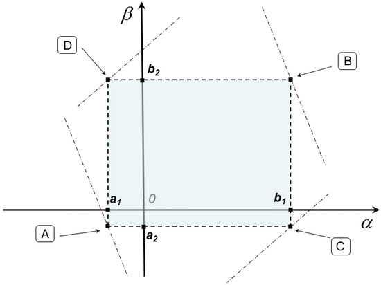
Proof of Lemma 1.

For the sake of simplicity, we refer to Figure 1. The objective function in (2) is continuous, so that the existence of solutions follows from the compactness and nonemptiness of the feasible region. In this regard, the compactness is a consequence of assuming $a_1,b_1,a_2,b_2$ finite. Furthermore, it is not difficult to realize that the feasible set of (2) is nonempty as long as at least one among the five conditions, Cond. I–Cond. V, is fulfilled, where the dashed-dotted line in Figure 1 represents the line associated with the last inequality constraint in (2). In particular, Cond. IV refers to the corner points A and B of Figure 1, while Cond. V refers to the vertices C and D. □

Figure 1. A graphical representation of the feasible set in (2). The dashed-dotted lines represent all the extreme choices for the last inequality constraint in (2).

3. On the Use of Quadratic Sub-Problems Within TRMs and LBMs, in Large-Scale Optimization

Here, we give details about a possible motivation for our proposal, in order to reduce the gap between two renowned classes of optimization methods, namely TRMs and LBMs. We are indeed persuaded that such a viewpoint may suggest a number of possible enhancements, to improve both the last classes of methods.

In this regard, observe that a TRM for large-scale problems is an iterative procedure that generates the sequence of n-real iterates $\left\{x_k\right\}$, and seeks at any step k for the solution of the trust-region sub-problem

$$\begin{array}{c}{\displaystyle \underset{s}{min}{q}_k\left(s\right)=f\left(x_k\right)+\nabla f{\left(x_k\right)}^{T}s+\frac{1}{2}{s}^T{Q}_{k}s}\hfill \\ {\parallel s\parallel }_2\le {\Delta }_k,\hfill \end{array}$$

(4)

where $x_k$ is the current iterate, $Q_k$ represents the exact/approximate Hessian matrix ${\nabla }^{2}f\left(x_k\right)$, and ${\Delta }_k>0$ represents the radius of the trust-region, i.e., the compact subset where the model $q_k\left(s\right)$ needs to be validated (for an exhaustive description of TRMs for Nonlinear Programming, the reader can refer to [2]). A number of possible variants of (4) can be introduced when n is large, including iterative updating strategies for both $Q_k$ and ${\Delta }_k$, and a number of approximate/sophisticated/refined schemes for its solution are available in the literature.

A distinguishing feature of TRMs, with respect to LBMs, is that at iteration k the methods in the first class attempt to determine the stepsize ${\alpha }_k$ and the search direction $d_k$ at once, so that $x_{k+1}=x_k+s_k\equiv x_k+{\alpha }_k{d}_k$, where $s_k$ indeed approximately/exactly solves (4). Conversely, in LBMs, the computations of ${\alpha }_k$ and $d_k$ are independent, as detailed later on in this paper. In particular, (see also [3]) the effective computation of $s_k$ in TRMs properly attempts to comply with the following issues:

• $s_k$ can be computed by either an exact (small- and medium-scale problems) or an approximate (large-scale problems) procedure;
• In order to prove the global convergence of the sequence $\left\{x_k\right\}$ to stationary limit points satisfying either first- or second-order necessary optimality conditions, $s_k$ is required to provide a sufficient reduction of the quadratic model $q_k\left(s\right)$, i.e., the difference $q_k\left(0\right)-q_k\left(s_k\right)$ is asked to satisfy a condition like ($c>0$)

  $$q_k\left(0\right)-q_k\left(s_k\right)\ge c{\parallel \nabla f\left(x_k\right)\parallel }_{2}min\left\{{\Delta }_k,{\displaystyle \frac{\parallel \nabla f\left(x_k\right){\parallel }_2}{1+{\parallel Q\parallel }_2}}\right\};$$
• $s_k$ can be computed by an approximate procedure, e.g., by adopting a Cauchy step or using the Steihaug conjugate gradient (see [22,23]), regardless of $Q_k$ signature. Then, the approximate solution of (4) is merely sought on a linear manifold of a dimension of one or at most two, rather than on the entire subset $B\equiv \{s\in {\mathbb{R}}^n:\parallel s{\parallel }_2\le {\Delta }_k\}$;
• Depending on a number of additional assumptions, TRMs can prove to be globally convergent to either a simple stationary limit point, or to a point which satisfies second-order necessary optimality conditions [2];
• Finding the exact/accurate solution of the sub-problem (4) is in general quite a cumbersome task in large-scale problems, representing a difficult goal that is often (when possible) skipped.

On the other hand, to some extent, LBMs represent the counterpart of TRMs. Indeed, to yield the next iterate $x_{k+1}=x_k+{\alpha }_k{d}_k$, they perform the computation of the steplength ${\alpha }_k$ and the direction $d_k$ as separate tasks. Furthermore, unlike for TRMs, the novel iterate $x_{k+1}$ in LBMs can be also obtained by adopting the more general update

$$x_{k+1}=x_k+{\alpha }_k{d}_k+{\beta }_k{z}_k,$$

(5)

with $d_k$ and $z_k$ now being two search directions summarizing different information on the function $f\left(x\right)$, and ${\alpha }_k$ and ${\beta }_k$ being stepsizes. In particular:

• when $z_k\equiv 0$ (or ${\beta }_k\equiv 0$ for any k), then $d_k$ represents a Newton-type direction, being typically computed by approximately solving Newton’s equation ${\nabla }^{2}f\left(x_k\right)d=-\nabla f\left(x_k\right)$ at the current iterate $x_k$. Then, an Armijo-type linesearch procedure is applied along $d_k$ to compute ${\alpha }_k$, provided that $d_k$ is gradient-related (see e.g., [3]) at $x_k$;
• when $z_k\ne 0$, then $d_k$ represents a Newton-type direction again, while $z_k$ is typically a negative curvature direction for $f\left(x\right)$ at $x_k$, which approximates an eigenvector associated with the least negative eigenvalue of ${\nabla }^{2}f\left(x_k\right)$. The vector $z_k$ plays an essential role, when LBMs’ convergence to stationary points satisfying the second-order necessary optimality conditions needs to be proved. In the last case, the computation of the steplengths ${\alpha }_k$ and ${\beta }_k$ is often carried out at once, (as in curvilinear linesearch procedures—see [24]), or the steplength computation is carried out by pursuing independent tasks (see, for example, [25]). We highlight that in (5), when both $d_k\ne 0$ and $z_k\ne 0$, we may experience difficulties related to properly scaling the two search directions.

As a general class of efficient algorithms within LBMs for large-scale problems, we find Truncated Newton methods (TNMs) coupled with a linesearch procedure (see Table 1). Similarly to general TRMs, they are evidently based on possibly computing $d_k$ and $z_k$ after exploiting the second-order Taylor’s expansion of $f\left(x\right)$ at $x_k$. However, a couple of quite disappointing issues arise when applying linesearch-based TNMs, namely:

• Unlike trust-region based TNMs, at iterate $x_k$, the search of a stationary point for a quadratic polynomial model of $f\left(x\right)$ (i.e., Newton’s equation) is performed on ${\mathbb{R}}^n$, so that the quadratic expansion is not trusted on a more reliable compact subset (trust-region) of ${\mathbb{R}}^n$. Thus, the search direction $d_k$ might show poor performance when the iterates in the sequence $\left\{x_k\right\}$ are far from a stationary limit point $x^{*}$. More specifically, note that in case ${\nabla }^{2}f\left(x_k\right)⪰0$; then, solving Newton’s equation and the trust-region sub-problem

  $$\begin{array}{c}{\displaystyle \underset{d}{min}{q}_k\left(d\right)=f\left(x_k\right)+\nabla f{\left(x_k\right)}^{T}d+\frac{1}{2}{d}^T{\nabla }^{2}f\left(x_k\right)d}\hfill \\ {\parallel d\parallel }_2\le {\gamma }_k,\hfill \end{array}$$

  for any ${\gamma }_k\ge {\parallel {\left[{\nabla }^{2}f\left(x_k\right)\right]}^{+}\nabla f\left(x_k\right)\parallel }_2$ yields the same solutions. Conversely, when ${\nabla }^{2}f\left(x_k\right)$ is indefinite, then Newton’s equation provides a saddle point for $q_k\left(d\right)$, that might be interpreted as a solution to a trust-region sub-problem (the interested reader may consider the paper [26] for some extensions). Furthermore, from this perspective, we remark that in LBMs, solving (2) where $d_k=-\nabla f\left(x_k\right)$, $z_k\equiv 0$, and ${\epsilon }_1={\epsilon }_2={\epsilon }_3=0$, is to a to large extent equivalent to computing the Cauchy step when solving (4). Indeed, in the last case, the trust-region constraint in (4), in principle, can be equivalently replaced by the compact feasible set (box constraints) in (2), after setting ${\epsilon }_1={\epsilon }_2={\epsilon }_3=0$. On the other hand, in case ${\nabla }^{2}f\left(x_k\right)⪰0$, and setting (2) $d_k=-\nabla f\left(x_k\right)$ and $z_k=-{\left[{\nabla }^{2}f\left(x_k\right)\right]}^{+}\nabla f\left(x_k\right)$, along with ${\epsilon }_1={\epsilon }_2={\epsilon }_3=0$, then, with similar reasoning, the solution to (2) closely resembles the application of the dogleg method when solving (4). Finally, since the coefficients $a_1,a_2$ in (2) may have negative values, we may potentially reverse the directions $d_k$ and $z_k$ when solving (2). Thus, following the idea behind (3), the scheme (2) suggests that, in case ${\nabla }^{2}f\left(x_k\right)$ is also indefinite, (2) easily generalizes the proposals in [27]. In fact, following (3), we are able to exactly compute a global minimum $({\alpha }^{*},{\beta }^{*})$ for (2), regardless of the signature of Q, so that the resulting direction ${\alpha }^{*}{d}_k+{\beta }^{*}{z}_k$ is gradient-related at $x_k$.
• As in (5), the search directions $d_k$ and $z_k$ might be suitably combined in a curvilinear framework (see, for example, [24]). However, to our knowledge, the selection of ${\alpha }_k$ and ${\beta }_k$ in the literature is seldom performed with a joint procedure to separately assess ${\alpha }_k$ and ${\beta }_k$, i.e., ${\alpha }_k$ and ${\beta }_k$ are rarely chosen as independent parameters. Hence, in the literature of linesearch-based TNMs, the linesearch procedure that starts from $x_k$ and yields $x_{k+1}$ explores a one-dimensional manifold (regular curve), rather than considering $x_k+\alpha d_k+\beta z_k$ as a two-dimensional manifold with independent real coefficients $\alpha$ and $\beta$.

In this regard, using (2) within LBMs tends to partially compensate for the drawbacks in the last two items, in light of the great success that TRMs have achieved in the last decade. In particular, using (2) within linesearch-based TNMs, our aim is that of developing a simple tool which could possibly carry out the following:

• Combines at iterate $x_k$ two independently computed vectors, namely $d_k,z_k\in {\mathbb{R}}^n$, by exactly computing a global minimum (we recall that, conversely, a global solution of the trust-region sub-problem (4) is often only approximately computed) for the two-dimensional constrained problem (2), being $\overline{x}\leftarrow x_k$, $d\leftarrow d_k$, $z\leftarrow z_k$;
• Adaptively updates the parameters $a_1$, $a_2$, $b_1$, $b_2$ in (2), when the iterate $x_k$ changes, following the rationale behind the update of ${\Delta }_k$ in (4), and retaining the strong convergence properties of TRMs. This fact is of remarkable interest, since in (2) the information associated with the search directions $d_k$ and $z_k$ is suitably trusted in a compact subset of ${\mathbb{R}}^n$ (namely, the box constraints $a_1\le \alpha \le b_1$, $a_2\le \beta \le b_2$);
• Exactly computes a cheap global minimum$({\alpha }^{*},{\beta }^{*})$ for (2), so that the vector ${\alpha }^{*}{d}_k+{\beta }^{*}{s}_k$ is then provided to a standard linesearch procedure such as the Armijo rule, to ensure that the global convergence of the sequence $\left\{x_k\right\}$ to stationary (limit) points is preserved;
• Allows for the convergence of subsequences of the iterates $\left\{x_k\right\}$ to stationary limit points, where either first- or second-order necessary optimality conditions are fulfilled;
• Preserves generality within a wide range of optimization frameworks, as reported in the next Section 4;
• Combines the effects of $d_k$ and $z_k$, skipping all the drawbacks related to a possible different scaling between these directions. We recall that since $d_k$ and $z_k$ are generated through the application of different methods, then the comparison of their performances may be biased by the latter generating methods.

• The TNMs sketched in Table 2, Table 3 and Table 4 are only examples of proposals in light of the previous comments.

4. How General Is the Model (2) in Nonlinear Programming Frameworks?

This section is devoted to reporting a number of real constrained optimization schemes from Nonlinear Programming, whose formulation is encompassed in (2). We can see that for some of the following schemes (see Figure 2), it is possible that more than one reformulation can be considered in the framework (2).

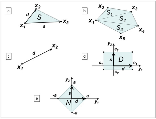
Figure 2. Examples where the structure of the feasible set in (2) is helpful: case (a) is treated in Section 4.1, case (b) is treated in Section 4.2, case (c) is treated in Section 4.3, case (d) is treated in Section 4.4 and case (e) is treated in Section 4.5.

4.1. Minimization over a Bounded Simplex

We consider the problem of minimizing a quadratic functional over the simplex $S\subset {\mathbb{R}}^n$, such that

$$\begin{array}{c}{\displaystyle \underset{x}{min}\frac{1}{2}{x}^{T}Qx+b^{T}x+c}\hfill \\ x\in S,\hfill \end{array}$$

(6)

where $S=\{x\in {\mathbb{R}}^n:x={\sum }_{i=1}^3{\lambda }_i{x}_i,{\sum }_{i=1}^3{\lambda }_i=1,{\lambda }_i\ge 0,i=1,2,3\}$. Figure 2a reports an example of a simplex. In this regard, by simply setting in (2)

• $d=x_2-x_1$, $z=x_3-x_1$,
• $\overline{x}=x_1$,
• $a_1=0$, $b_1=1$, $a_2=0$, $b_2=1$,
• ${ϵ}_1={ϵ}_2={ϵ}_3=1$,

• the problem (6) is a special case of the problem (2).

4.2. Minimization over a Bounded Polygon

We consider the problem of minimizing a quadratic functional over a polygon $P\subset {\mathbb{R}}^2$, described by a finite number m of vertices (observe that the points in the polygon P must belong to a hyperplane $\pi \subset {\mathbb{R}}^n$, with $\pi :{\omega }^{T}x+{\omega }_0=0$, $\omega ={({\omega }_1,\dots ,{\omega }_n)}^T\in {\mathbb{R}}^n$, ${\omega }_0\in \mathbb{R}$, so that ${\omega }^T\overline{x}+{\omega }_0=0$ for any $\overline{x}\in P$.), i.e.,

$$\begin{array}{c}{\displaystyle \underset{x}{min}\frac{1}{2}{x}^{T}Qx+b^{T}x+c}\hfill \\ x\in P,\hfill \end{array}$$

(7)

where $P=\{x\in {\mathbb{R}}^2:x={\sum }_{i=1}^m{\lambda }_i{x}_i,{\sum }_{i=1}^m{\lambda }_i=1,{\lambda }_i\ge 0,i=1,\dots ,m\}$. Figure 2b reports an example of a polygon with $m=5$. In this regard, the problem (7) can be split into to solution of the $(m-2)$ sub-problems

$$\begin{array}{c}{\displaystyle \underset{x}{min}\frac{1}{2}{x}^{T}Qx+b^{T}x+c}\hfill \\ x\in S_i,i=1,\dots ,m-2,\hfill \end{array}$$

(8)

where

$$\begin{array}{c}{S}_i=\left\{x\in \pi \subset {\mathbb{R}}^2:x={\displaystyle \sum _{j\in \{1,i+1,i+2\}}}{\lambda }_j{x}_j,{\displaystyle \sum _{j\in \{1,i+1,i+2\}}}{\lambda }_j=1,{\lambda }_j\ge 0,j\in \{1,i+1,i+2\}\right\},\end{array}$$

which are of the form (6). Thus, solving the problem (7) corresponds to solve a sequence of $(m-2)$ instances of the problem (2).

4.3. Minimization over a Bounded Segment

We consider the problem of minimizing a quadratic functional over a segment $L\subset {\mathbb{R}}^n$, i.e.,

$$\begin{array}{c}{\displaystyle \underset{x}{min}\frac{1}{2}{x}^{T}Qx+b^{T}x+c}\hfill \\ x\in L,\hfill \end{array}$$

(9)

where $L=\{x\in {\mathbb{R}}^n:x=\lambda x_1+(1-\lambda )x_2,\lambda \in [0,1]\}$. Figure 2c reports an example of a segment. In this regard, by simply setting in (2)

• $d=x_2-x_1$, $z\equiv 0$,
• $\overline{x}=x_1$,
• $a_1=0$, $b_1=1$, $a_2=0$, $b_2=0$,
• ${ϵ}_1={ϵ}_2={ϵ}_3=0$,

• the problem (9) is a special case of the problem (2).

4.4. Minimization over a Bounded Box in ${\mathbb{R}}^2$

We consider the problem of minimizing a quadratic functional over a box domain $D\subset {\mathbb{R}}^2$, i.e.,

$$\begin{array}{c}{\displaystyle \underset{x}{min}\frac{1}{2}{x}^{T}Qx+b^{T}x+c}\hfill \\ x\in D,\hfill \end{array}$$

(10)

where $D=\{x\in {\mathbb{R}}^2:c_i\le x_i\le e_i,i=1,2\}$. Figure 2d reports an example of a box domain. In this regard, by simply setting in (2)

• $d=\left(\begin{array}{c}{e}_1-c_1\\ 0\end{array}\right)$, $z=\left(\begin{array}{c}0\\ e_2-c_2\end{array}\right)$
• $\overline{x}=\left(\begin{array}{c}{c}_1\\ c_2\end{array}\right)$
• $a_1=0$, $b_1=1$, $a_2=0$, $b_2=1$,
• ${ϵ}_1={ϵ}_2={ϵ}_3=0$,

• the problem (10) is a special case of the problem (2). As an alternative to the previous setting, we might also consider treating this case with a setting in (2), given by

• $d=\left(\begin{array}{c}{\displaystyle \frac{e_1-c_1}{2}}\\ 0\end{array}\right)$, $z=\left(\begin{array}{c}0\\ {\displaystyle \frac{e_2-c_2}{2}}\end{array}\right)$
• $\overline{x}=\left(\begin{array}{c}{\displaystyle \frac{e_1+c_1}{2}}\\ {\displaystyle \frac{e_2+c_2}{2}}\end{array}\right)$
• $a_1=-1$, $b_1=1$, $a_2=-1$, $b_2=1$,
• ${ϵ}_1={ϵ}_2={ϵ}_3=0$.

4.5. Minimization Including a 1-Norm Inequality Constraint in ${\mathbb{R}}^2$

We consider the problem of minimizing a quadratic functional subject to the 1-norm inequality constraint $x\in N$, with $N\subset {\mathbb{R}}^2$, i.e.,

$$\begin{array}{c}{\displaystyle \underset{x}{min}\frac{1}{2}{x}^{T}Qx+b^{T}x+c}\hfill \\ x\in N,\hfill \end{array}$$

(11)

which is $N=\{x\in {\mathbb{R}}^2:\parallel x{\parallel }_1\le a\}$. Figure 2e reports an example of such a constraint. In this regard, it suffices to recast (11) as in (8), where

• $m=6$
• $\overline{x}=x_1=0$
• $x_2=\left(\begin{array}{c}0\\ 1\end{array}\right)$, $x_3=\left(\begin{array}{c}1\\ 0\end{array}\right)$, $x_4=\left(\begin{array}{c}0\\ -1\end{array}\right)$, $x_5=\left(\begin{array}{c}-1\\ 0\end{array}\right)$, $x_6=x_2$,

• so that four instances of the problem (2) need to be solved.

4.6. Minimization Including an ∞-Norm Inequality Constraint in ${\mathbb{R}}^2$

We consider the problem of minimizing a quadratic functional subject to the ∞-norm inequality constraint $x\in E$, with $E\subset {\mathbb{R}}^2$, i.e.,

$$\begin{array}{c}{\displaystyle \underset{x}{min}\frac{1}{2}{x}^{T}Qx+b^{T}x+c}\hfill \\ x\in E,\hfill \end{array}$$

(12)

which is $E=\{x\in {\mathbb{R}}^2:\parallel x{\parallel }_{\infty }\le a\}$. In this regard, we obtain similar results with respect to Section 4.5. Indeed, by simply setting in (2)

• $d=\left(\begin{array}{c}a\\ 0\end{array}\right)$, $z=\left(\begin{array}{c}0\\ a\end{array}\right)$
• $\overline{x}=0$
• $a_1=-1$, $b_1=1$, $a_2=-1$, $b_2=1$,
• ${ϵ}_1={ϵ}_2={ϵ}_3=0$,

• the problem (12) is a special case of the problem (2).

4.7. Minimization Including a 2-Norm Inequality Constraint in ${\mathbb{R}}^2$

We consider the problem of minimizing a quadratic functional in ${\mathbb{R}}^2$ subject to the 2-norm inequality constraint ${\parallel x\parallel }_2\le \gamma$, with $\gamma \ge 0$, i.e.,

$$\begin{array}{c}{\displaystyle \underset{x}{min}\frac{1}{2}{x}^{T}Qx+b^{T}x+c}\hfill \\ {\parallel x\parallel }_2\le \gamma ,x\in {\mathbb{R}}^2.\hfill \end{array}$$

(13)

In this regard, it suffices to observe that the solution of (2) provides both a

• LOWER bound to the solution of (13), as long as we set (following Section 4.6)

  – 

  $d=\left(\begin{array}{c}\gamma \\ 0\end{array}\right)$, $z=\left(\begin{array}{c}0\\ \gamma \end{array}\right)$

  – 

  $\overline{x}=0$

  – 

  $a_1=-1$, $b_1=1$, $a_2=-1$, $b_2=1$,

  – 

  ${ϵ}_1={ϵ}_2={ϵ}_3=0$,

• UPPER bound: to the solution of (13), as long as we follow the indications in Section 4.5, i.e., we recast and solve (11) as in (8), where

  – 

  $m=6$

  – 

  $\overline{x}=x_1=0$

  – 

  $x_2=\left(\begin{array}{c}0\\ \gamma \end{array}\right)$, $x_3=\left(\begin{array}{c}\gamma \\ 0\end{array}\right)$, $x_4=\left(\begin{array}{c}0\\ -\gamma \end{array}\right)$, $x_5=\left(\begin{array}{c}-\gamma \\ 0\end{array}\right)$, $x_6=x_2$,

  so that four instances of the problem (2) need to be solved.

Note that the dogleg-like methods for the approximate solution of the trust-region problem (4), in the convex case, equivalently solve the sub-problem (13) with just a couple of unknowns.

5. KKT Conditions and the Fast Solution of Problem (2)

Replacing the expression of the vector x in (2) within the objective function, we easily obtain the equivalent problem

$$\begin{array}{c}{\displaystyle \underset{\alpha ,\beta }{min}\phi (\alpha ,\beta )}\hfill \\ \mathcal{P}:\left\{\begin{array}{c}{a}_1\le \alpha \le b_1\hfill \\ a_2\le \beta \le b_2\hfill \\ {ϵ}_1\alpha +{ϵ}_2\beta \le {ϵ}_3,\hfill \end{array}\right.\hfill \end{array}$$

(14)

where

$$\left\{\begin{array}{c}\phi (\alpha ,\beta )={\displaystyle \frac{1}{2}}{\left(\begin{array}{c}\alpha \\ \beta \end{array}\right)}^T\left(\begin{array}{cc}t& u\\ u& w\end{array}\right)\left(\begin{array}{c}\alpha \\ \beta \end{array}\right)+{\left(\begin{array}{c}y\\ h\end{array}\right)}^T\left(\begin{array}{c}\alpha \\ \beta \end{array}\right)+q\hfill \\ t=d^{T}Qd\hfill \\ u=d^{T}Qz=z^{T}Qd\hfill \\ w=z^{T}Qz\hfill \\ y={(Q\overline{x}+b)}^{T}d\hfill \\ h={(Q\overline{x}+b)}^{T}z\hfill \\ q={\left({\displaystyle \frac{1}{2}}Q\overline{x}+b\right)}^T\overline{x}+c.\hfill \end{array}\right.$$

Observe that transforming (2) into (14) only requires the computation of two additional matrix-vector products (i.e., $Qd$ and $Qz$), along with six inner products. The problem (14) is a constrained quadratic problem, such that first-order Fritz-John optimality conditions do not require additional constraint qualifications (since all the constraints are linear). Thus, after considering its Lagrangian function

$$\begin{array}{ccc}\hfill \mathcal{L}(\alpha ,\beta ,{\mu }_1,{\mu }_2,{\mu }_3,{\mu }_4,{\mu }_5)& =& \\ & & \phi (\alpha ,\beta )-{\mu }_1(\alpha -a_1)+{\mu }_2(\alpha -b_1)-{\mu }_3(\beta -a_2)+{\mu }_4(\beta -b_2)+{\mu }_5({ϵ}_1\alpha +{ϵ}_2\beta -{ϵ}_3)\hfill \end{array}$$

we have the next set of equalities/inequalities representing the associated KKT conditions:

$$\left\{\begin{array}{c}\left(\begin{array}{cc}t& u\\ u& w\end{array}\right)\left(\begin{array}{c}{\alpha }^{*}\\ {\beta }^{*}\end{array}\right)+\left(\begin{array}{c}y\\ h\end{array}\right)+\left(\begin{array}{c}-{\mu }_1^{*}+{\mu }_2^{*}+{ϵ}_1{\mu }_5^{*}\\ -{\mu }_3^{*}+{\mu }_4^{*}+{ϵ}_2{\mu }_5^{*}\end{array}\right)=\left(\begin{array}{c}0\\ 0\end{array}\right)\hfill \\ \left(\begin{array}{c}{\alpha }^{*}\\ {\beta }^{*}\end{array}\right)\in \mathcal{P}\hfill \\ {\mu }_1^{*}[{\alpha }^{*}-a_1]=0\hfill \\ {\mu }_2^{*}[{\alpha }^{*}-b_1]=0\hfill \\ {\mu }_3^{*}[{\beta }^{*}-a_2]=0\hfill \\ {\mu }_4^{*}[{\beta }^{*}-b_2]=0\hfill \\ {\mu }_5^{*}[{ϵ}_1{\alpha }^{*}+{ϵ}_2{\beta }^{*}-{ϵ}_3]=0\hfill \\ {\mu }_i^{*}\ge 0,i=1,\dots ,5.\hfill \end{array}\right.$$

(15)

The remaining part of the present section will be devoted to analyze all the possible solutions of (15), with the aim of possibly computing a global minimum for (2). In this regard, exploiting the solutions of (15) evidently undergoes a reduction, allowing us to analyze the cases (I)–(XII) in Figure 3.

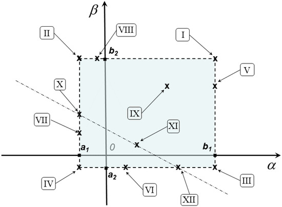
Figure 3. Overview of possible solutions (I)–(XII) for KKT conditions in (15).

Observing that in (15) the multipliers ${\mu }_i^{*}$ and $i=1,\dots ,5$ must fulfill nonnegativity conditions, it is not difficult to realize that computing all the KKT points satisfying (15) can turn out to be a burdensome task, including a number of sub-cases depending on the possible combinations of signs for the parameters $a_1$, $b_1$, $a_2$, $b_2$, ${ϵ}_1$, ${ϵ}_2$ and ${ϵ}_3$. Conversely, a global minimizer for (2) can be equivalently exploited by analyzing all the possible solutions of (15) uniquely in terms of ${\alpha }^{*}$ and ${\beta }^{*}$, without requiring the computation of the multipliers as well. Hence, we limit our analysis to consider the computation of ${\alpha }^{*}$ and ${\beta }^{*}$ in the cases (I)–(XII) of Figure 3, where

• Cases (I), (II), (III), (IV) are associated with possible solutions in the vertices of the box constraints;
• Cases (V), (VI), (VII), (VIII) are associated with possible solutions on the edges of the box constraints;
• Case (IX) represents a possible feasible unconstrained minimizer for the objective function in (2);
• Cases (X), (XI), (XII) are associated with possible solutions, making the last inequality constraint in (14) active.

Then, in Lemma 2, we will provide a simple theoretical result which justifies our simplification, with respect to computing all the KKT points. In this regard, we preliminarily set $i=1$ and consider the next cases from Figure 3, with $\left\{y_i\right\}$ being the sequence of tentative solution points of (14):

• Case (I): We set $\overline{\alpha }=b_1$, $\overline{\beta }=b_2$. If $\boxed{{ϵ}_1\overline{\alpha }+{ϵ}_2\overline{\beta }\le {ϵ}_3}$, then set

  $$P_1=\left(\begin{array}{c}{b}_1\\ b_2\end{array}\right),{\phi }_i=\phi (b_1,b_2),y_i=P_1,i=i+1;$$

  (16)
• Case (II): We set $\overline{\alpha }=a_1$, $\overline{\beta }=b_2$. If $\boxed{{ϵ}_1\overline{\alpha }+{ϵ}_2\overline{\beta }\le {ϵ}_3}$, then set

  $$P_2=\left(\begin{array}{c}{a}_1\\ b_2\end{array}\right),{\phi }_i=\phi (a_1,b_2),y_i=P_2,i=i+1;$$

  (17)
• Case (III): We set $\overline{\alpha }=b_1$, $\overline{\beta }=a_2$. If $\boxed{{ϵ}_1\overline{\alpha }+{ϵ}_2\overline{\beta }\le {ϵ}_3}$, then set

  $$P_3=\left(\begin{array}{c}{b}_1\\ a_2\end{array}\right),{\phi }_i=\phi (b_1,a_2),y_i=P_3,i=i+1;$$

  (18)
• Case (IV): We set $\overline{\alpha }=a_1$, $\overline{\beta }=a_2$. If $\boxed{{ϵ}_1\overline{\alpha }+{ϵ}_2\overline{\beta }\le {ϵ}_3}$, then set

  $$P_4=\left(\begin{array}{c}{a}_1\\ a_2\end{array}\right),{\phi }_i=\phi (a_1,a_2),y_i=P_4,i=i+1;$$

  (19)
• Case (V): We set $\overline{\alpha }=b_1$ and possibly compute the solution $\overline{\beta }=-(u{b}_1+h)/w$ of the equation

  $${\displaystyle \frac{d\phi (b_1,\beta )}{d\beta }}=w\beta +u{b}_1+h=0,$$

  so that:

  – 

  if $\boxed{w\ne 0 \mathrm{AND} {ϵ}_1\overline{\alpha }+{ϵ}_2\overline{\beta }\le {ϵ}_3}$, then set

  $$P_5=\left(\begin{array}{c}\overline{\alpha }\\ \overline{\beta }\end{array}\right),{\phi }_i=\phi \left(\overline{\alpha },\overline{\beta }\right),y_i=P_5,i=i+1;$$

  (20)

  – 

  if $\boxed{w=0 \mathrm{AND} u{b}_1+h\ne 0}$, then there is no solution for Case (V);

  – 

  if $\boxed{w=0 \mathrm{AND} u{b}_1+h=0}$, then set $\overline{\beta }\in [a_2,b_2]$ as any value satisfying ${ϵ}_1\overline{\alpha }+{ϵ}_2\overline{\beta }\le {ϵ}_3$, and compute $P_5$ as in (20);

• Case (VI): We set $\overline{\beta }=a_2$ and possibly compute the solution $\overline{\alpha }=-(u{a}_2+y)/t$ of the equation

  $${\displaystyle \frac{d\phi (\alpha ,a_2)}{d\alpha }}=t\alpha +u{a}_2+y=0,$$

  so that:

  – 

  if $\boxed{t\ne 0 \mathrm{AND} {ϵ}_1\overline{\alpha }+{ϵ}_2\overline{\beta }\le {ϵ}_3}$, then set

  $$P_6=\left(\begin{array}{c}\overline{\alpha }\\ \overline{\beta }\end{array}\right),{\phi }_i=\phi (\overline{\alpha },\overline{\beta }),y_i=P_6,i=i+1;$$

  (21)

  – 

  if $\boxed{t=0 \mathrm{AND} u{a}_2+y\ne 0}$, then there is no solution for Case (VI);

  – 

  if $\boxed{t=0 \mathrm{AND} u{a}_2+y=0}$, then set $\overline{\alpha }\in [a_1,b_1]$ as any value satisfying ${ϵ}_1\overline{\alpha }+{ϵ}_2\overline{\beta }\le {ϵ}_3$, and compute $P_6$ as in (21);

• Case (VII): We set $\overline{\alpha }=a_1$ and possibly compute the solution $\overline{\beta }=-(u{a}_1+z)/w$ of the equation

  $${\displaystyle \frac{d\phi (a_1,\beta )}{d\beta }}=w\beta +u{a}_1+h=0,$$

  so that:

  – 

  if $\boxed{w\ne 0 \mathrm{AND} {ϵ}_1\overline{\alpha }+{ϵ}_2\overline{\beta }\le {ϵ}_3}$, then set

  $$P_7=\left(\begin{array}{c}\overline{\alpha }\\ \overline{\beta }\end{array}\right),{\phi }_i=\phi (\overline{\alpha },\overline{\beta }),y_i=P_7,i=i+1;$$

  (22)

  – 

  if $\boxed{w=0 \mathrm{AND} u{a}_1+h\ne 0}$, then there is no solution for Case (VII);

  – 

  if $\boxed{w=0 \mathrm{AND} u{a}_1+h=0}$, then set $\overline{\beta }\in [a_2,b_2]$ as any value satisfying ${ϵ}_1\overline{\alpha }+{ϵ}_2\overline{\beta }\le {ϵ}_3$, and compute $P_7$ as in (22);

• Case (VIII): We set $\overline{\beta }=b_2$ and possibly compute the solution $\overline{\alpha }=-(u{b}_2+y)/t$ of the equation

  $${\displaystyle \frac{d\phi (\alpha ,b_2)}{d\alpha }}=t\alpha +u{b}_2+y=0,$$

  so that:

  – 

  if $\boxed{t\ne 0 \mathrm{AND} {ϵ}_1\overline{\alpha }+{ϵ}_2\overline{\beta }\le {ϵ}_3}$, then set

  $$P_8=\left(\begin{array}{c}\overline{\alpha }\\ \overline{\beta }\end{array}\right),{\phi }_i=\phi (\overline{\alpha },\overline{\beta }),y_i=P_8,i=i+1;$$

  (23)

  – 

  if $\boxed{t=0 \mathrm{AND} u{b}_2+y\ne 0}$, then there is no solution for Case (VIII);

  – 

  if $\boxed{t=0 \mathrm{AND} u{b}_2+y=0}$, then set $\overline{\alpha }\in [a_1,b_1]$ as any value satisfying ${ϵ}_1\overline{\alpha }+{ϵ}_2\overline{\beta }\le {ϵ}_3$, and compute $P_8$ as in (23);

• Case (IX): If $\boxed{tw-u^2\ne 0}$, we compute the solution

  $$\left(\begin{array}{c}\overline{\alpha }\\ \overline{\beta }\end{array}\right)=-{\left(\begin{array}{cc}t& u\\ u& w\end{array}\right)}^{-1}\left(\begin{array}{c}y\\ h\end{array}\right)$$

  of the linear system

  $$\left\{\begin{array}{c}{\phi }_{\alpha }(\alpha ,\beta )=t\alpha +u\beta +y=0\hfill \\ \hfill \\ {\phi }_{\beta }(\alpha ,\beta )=u\alpha +w\beta +h=0;\hfill \end{array}\right.$$

  otherwise, in case $\boxed{tw-u^2=0 \mathrm{AND} \left((th-uy\ne 0)\mathrm{OR}(uh-wy\ne 0)\right)}$, then there is no solution for Case (IX);
  otherwise, in case $\boxed{tw-u^2=0 \mathrm{AND} (th-uy=0) \mathrm{AND} (uh-wy=0)}$, then we have three sub-cases:
  • $\boxed{t>0}$: then, recalling that we are in the sub-case where equations ${\phi }_{\alpha }(\alpha ,\beta )=0$ and ${\phi }_{\beta }(\alpha ,\beta )=0$ yield the same information, we exploit equation ${\phi }_{\alpha }(\alpha ,\beta )=0$ and we set $\alpha =-(u\beta +y)/t$. Thus, from the bounds and the last inequality in (14), we obtain

    $$\left\{\begin{array}{c}{a}_2\le \beta \le b_2\hfill \\ \hfill \\ \left({\epsilon }_{2}t-{\epsilon }_{1}u\right)\beta \le {\epsilon }_{3}t+{\epsilon }_{1}y\hfill \\ \hfill \\ a_{1}t+y\le -u\beta \le b_{1}t+y\hfill \end{array}\right.$$

    which yield the next three cases:

    – 

    $\boxed{{\epsilon }_{2}t-{\epsilon }_{1}u>0}$: admitting other three sub-cases, namely

    ∗

    $\boxed{u>0}$, so that we set

    $${\beta }_1=max\left\{a_2,-{\displaystyle \frac{b_{1}t+y}{u}}\right\}\le \beta \le min\left\{b_2,{\displaystyle \frac{{\epsilon }_{3}t+{\epsilon }_{1}y}{{\epsilon }_{2}t-{\epsilon }_{1}u}},-{\displaystyle \frac{a_{1}t+y}{u}}\right\}={\beta }_2$$

    ∗

    $\boxed{u=0}$, so that we set

    $${\beta }_1=a_2\le \beta \le min\left\{b_2,{\displaystyle \frac{{\epsilon }_{3}t+{\epsilon }_{1}y}{{\epsilon }_{2}t}}\right\}={\beta }_2$$

    ∗

    $\boxed{u<0}$, so that we set

    $${\beta }_1=max\left\{a_2,-{\displaystyle \frac{a_{1}t+y}{u}}\right\}\le \beta \le min\left\{b_2,{\displaystyle \frac{{\epsilon }_{3}t+{\epsilon }_{1}y}{{\epsilon }_{2}t-{\epsilon }_{1}u}},-{\displaystyle \frac{b_{1}t+y}{u}}\right\}={\beta }_2$$

    – 

    $\boxed{{\epsilon }_{2}t-{\epsilon }_{1}u=0}$: admitting no solution for Case (IX) as long as the condition $\boxed{{\epsilon }_{3}t+{\epsilon }_{1}y<0}$ holds. Conversely, in case $\boxed{{\epsilon }_{3}t+{\epsilon }_{1}y\ge 0}$, we have the three cases:

    ∗

    $\boxed{u>0}$, so that we set

    $${\beta }_1=max\left\{a_2,-{\displaystyle \frac{b_{1}t+y}{u}}\right\}\le \beta \le min\left\{b_2,-{\displaystyle \frac{a_{1}t+y}{u}}\right\}={\beta }_2$$

    ∗

    $\boxed{u=0}$, so that we set

    $${\beta }_1=a_2\le \beta \le b_2={\beta }_2$$

    ∗

    $\boxed{u<0}$, so that we set

    $${\beta }_1=max\left\{a_2,-{\displaystyle \frac{a_{1}t+y}{u}}\right\}\le \beta \le min\left\{b_2,-{\displaystyle \frac{b_{1}t+y}{u}}\right\}={\beta }_2$$

    – 

    $\boxed{{\epsilon }_{2}t-{\epsilon }_{1}u<0}$: corresponding to the three cases:

    ∗

    $\boxed{u>0}$, so that we set

    $${\beta }_1=max\left\{a_2,-{\displaystyle \frac{b_{1}t+y}{u}},{\displaystyle \frac{{\epsilon }_{3}t+{\epsilon }_{1}y}{{\epsilon }_{2}t-{\epsilon }_{1}u}}\right\}\le \beta \le min\left\{b_2,-{\displaystyle \frac{a_{1}t+y}{u}}\right\}={\beta }_2$$

    ∗

    $\boxed{u=0}$, so that we set

    $${\beta }_1=max\left\{a_2,{\displaystyle \frac{{\epsilon }_{3}t+{\epsilon }_{1}y}{{\epsilon }_{2}t-{\epsilon }_{1}u}}\right\}\le \beta \le b_2={\beta }_2$$

    ∗

    $\boxed{u<0}$, so that we set

    $${\beta }_1=max\left\{a_2,-{\displaystyle \frac{a_{1}t+y}{u}},{\displaystyle \frac{{\epsilon }_{3}t+{\epsilon }_{1}y}{{\epsilon }_{2}t-{\epsilon }_{1}u}}\right\}\le \beta \le min\left\{b_2,-{\displaystyle \frac{b_{1}t+y}{u}}\right\}={\beta }_2$$

  • $\boxed{t=0}$: then, recalling that we are in the sub-case where equations ${\phi }_{\alpha }(\alpha ,\beta )=0$ and ${\phi }_{\beta }(\alpha ,\beta )=0$ yield the same information, with $tw-u^2=0$, we exploit equation ${\phi }_{\alpha }(\alpha ,\beta )=0$ with $t=u=0$. Therefore, we have

    $$\left\{\begin{array}{c}{a}_2\le \beta \le b_2\hfill \\ \hfill \\ y=0\hfill \\ \hfill \\ a_1\le \alpha \le b_1\hfill \end{array}\right.$$

    which yield the next two cases:

    – 

    $\boxed{y=0}$ This case implies that the objective function is constant (i.e., $\phi (\alpha ,\beta )=q$), so that we set

    $${\beta }_1=a_2\le \beta \le b_2={\beta }_2$$

    – 

    $\boxed{y\ne 0}$: admitting no solution for Case (IX)

  • $\boxed{t<0}$: then, recalling that we are again in the sub-case where equations ${\phi }_{\alpha }(\alpha ,\beta )=0$ and ${\phi }_{\beta }(\alpha ,\beta )=0$ yield the same information, we exploit equation ${\phi }_{\alpha }(\alpha ,\beta )=0$ and we set $\alpha =-(u\beta +y)/t$. Thus, from the bounds and the last inequality in (14), we obtain

    $$\left\{\begin{array}{c}{a}_2\le \beta \le b_2\hfill \\ \hfill \\ \left({\epsilon }_{2}t-{\epsilon }_{1}u\right)\beta \ge {\epsilon }_{3}t+{\epsilon }_{1}y\hfill \\ \hfill \\ b_{1}t+y\le -u\beta \le a_{1}t+y\hfill \end{array}\right.$$

    which yield the next three cases:

    – 

    $\boxed{{\epsilon }_{2}t-{\epsilon }_{1}u>0}$: admitting other three cases, namely

    ∗

    $\boxed{u>0}$, so that we set

    $${\beta }_1=max\left\{a_2,-{\displaystyle \frac{a_{1}t+y}{u}},{\displaystyle \frac{{\epsilon }_{3}t+{\epsilon }_{1}y}{{\epsilon }_{2}t-{\epsilon }_{1}u}}\right\}\le \beta \le min\left\{b_2,-{\displaystyle \frac{b_{1}t+y}{u}}\right\}={\beta }_2$$

    ∗

    $\boxed{u=0}$, so that $b_{1}t+y\le -u\beta \le a_{1}t+y$ is always fulfilled and we set

    $${\beta }_1=max\left\{a_2,{\displaystyle \frac{{\epsilon }_{3}t+{\epsilon }_{1}y}{{\epsilon }_{2}t}}\right\}\le \beta \le b_2={\beta }_2$$

    ∗

    $\boxed{u<0}$, so that we set

    $${\beta }_1=max\left\{a_2,-{\displaystyle \frac{b_{1}t+y}{u}},{\displaystyle \frac{{\epsilon }_{3}t+{\epsilon }_{1}y}{{\epsilon }_{2}t-{\epsilon }_{1}u}}\right\}\le \beta \le min\left\{b_2,-{\displaystyle \frac{a_{1}t+y}{u}}\right\}={\beta }_2$$

    – 

    $\boxed{{\epsilon }_{2}t-{\epsilon }_{1}u=0}$: admitting no solution for Case (IX) as long as the condition $\boxed{{\epsilon }_{3}t+{\epsilon }_{1}y>0}$ holds. Conversely, in case $\boxed{{\epsilon }_{3}t+{\epsilon }_{1}y\le 0}$ we have the three cases:

    ∗

    $\boxed{u>0}$, so that we set

    $${\beta }_1=max\left\{a_2,-{\displaystyle \frac{a_{1}t+y}{u}}\right\}\le \beta \le min\left\{b_2,-{\displaystyle \frac{b_{1}t+y}{u}}\right\}={\beta }_2$$

    ∗

    $\boxed{u=0}$, so that we set

    $${\beta }_1=a_2\le \beta \le b_2={\beta }_2$$

    ∗

    $\boxed{u<0}$, so that we set

    $${\beta }_1=max\left\{a_2,-{\displaystyle \frac{b_{1}t+y}{u}}\right\}\le \beta \le min\left\{b_2,-{\displaystyle \frac{a_{1}t+y}{u}}\right\}={\beta }_2$$

    – 

    $\boxed{{\epsilon }_{2}t+{\epsilon }_{1}u<0}$: corresponding to the three cases

    ∗

    $\boxed{u>0}$, so that we set

    $${\beta }_1=max\left\{a_2,-{\displaystyle \frac{a_{1}t+y}{u}}\right\}\le \beta \le min\left\{b_2,{\displaystyle \frac{{\epsilon }_{3}t+{\epsilon }_{1}y}{{\epsilon }_{2}t-{\epsilon }_{1}u}},-{\displaystyle \frac{b_{1}t+y}{u}}\right\}={\beta }_2$$

    ∗

    $\boxed{u=0}$, so that we set

    $${\beta }_1=a_2\le \beta \le min\left\{b_2,{\displaystyle \frac{{\epsilon }_{3}t+{\epsilon }_{1}y}{{\epsilon }_{2}t-{\epsilon }_{1}u}}\right\}={\beta }_2$$

    ∗

    $\boxed{u<0}$, so that we set

    $${\beta }_1=max\left\{a_2,-{\displaystyle \frac{b_{1}t+y}{u}}\right\}\le \beta \le min\left\{b_2,{\displaystyle \frac{{\epsilon }_{3}t+{\epsilon }_{1}y}{{\epsilon }_{2}t-{\epsilon }_{1}u}},-{\displaystyle \frac{a_{1}t+y}{u}}\right\}={\beta }_2.$$

  Thus, overall, for Case (IX), if ${\beta }_1\le {\beta }_2$, we set

  $$\overline{\beta }=({\beta }_1+{\beta }_2)/2,\overline{\alpha }=\left\{\begin{array}{ccc}-(u\overline{\beta }+y)/t\hfill & & t\ne 0\hfill \\ (a_1+b_1)/2\hfill & & t=0,\hfill \end{array}\right.$$

  along with

  $$\begin{array}{c}{P}_9=\left(\begin{array}{c}\overline{\alpha }\\ \overline{\beta }\end{array}\right),{\phi }_i=\phi (\overline{\alpha },\overline{\beta }),y_i=P_9,i=i+1,\hfill \end{array}$$

  (24)

  otherwise, if ${\beta }_1>{\beta }_2$, there is no solution for Case (IX);
• Case (X): We set $\overline{\alpha }=a_1$ with ${\epsilon }_1{a}_1+{\epsilon }_2\beta ={\epsilon }_3$, and we distinguish among three cases:

  – 

  if $\boxed{{\epsilon }_2=0 \mathrm{AND} {\epsilon }_3={\epsilon }_1{a}_1}$, then set ${\beta }_1=a_2\le \beta \le b_2={\beta }_2$;

  – 

  if $\boxed{{\epsilon }_2=0 \mathrm{AND} {\epsilon }_3\ne {\epsilon }_1{a}_1}$, then there is no solution for Case (X);

  – 

  if $\boxed{{\epsilon }_2\ne 0}$, then set

  $${\beta }_1=max\left\{a_2,{\displaystyle \frac{{\epsilon }_3-{\epsilon }_1{a}_1}{{\epsilon }_2}}\right\}\le \beta \le min\left\{b_2,{\displaystyle \frac{{\epsilon }_3-{\epsilon }_1{a}_1}{{\epsilon }_2}}\right\}={\beta }_2.$$

  Set $\overline{\beta }=({\beta }_1+{\beta }_2)/2$ with

  $$P_{10}=\left(\begin{array}{c}{a}_1\\ \overline{\beta }\end{array}\right),{\phi }_i=\phi (a_1,\overline{\beta }),y_i=P_{10},i=i+1;$$

  (25)
• Case (XI): We distinguish among the next four cases:

  – 

  if $\boxed{{\epsilon }_1={\epsilon }_2=0 \mathrm{AND} {\epsilon }_3\ge 0}$, then set $\overline{\alpha }=(a_1+b_1)/2$, ${\beta }_1=a_2\le \beta \le {\beta }_2=b_2$; otherwise, there is no solution for Case (XI);

  – 

  if $\boxed{{\epsilon }_1>0}$, then $\alpha =(-{\epsilon }_2\beta +{\epsilon }_3)/{\epsilon }_1$ and we analyze three sub-cases:

  • If $\boxed{{\epsilon }_2>0}$, then set

    $${\beta }_1=max\left\{a_2,{\displaystyle \frac{{\epsilon }_1{b}_1-{\epsilon }_3}{-{\epsilon }_2}}\right\}\le \beta \le min\left\{b_2,{\displaystyle \frac{{\epsilon }_1{a}_1-{\epsilon }_3}{-{\epsilon }_2}}\right\}={\beta }_2;$$
  • If $\boxed{{\epsilon }_2=0}$, then set ${\beta }_1=a_2\le \beta \le b_2={\beta }_2$;
  • If $\boxed{{\epsilon }_2<0}$, then set

    $${\beta }_1=max\left\{a_2,{\displaystyle \frac{{\epsilon }_1{a}_1-{\epsilon }_3}{-{\epsilon }_2}}\right\}\le \beta \le min\left\{b_2,{\displaystyle \frac{{\epsilon }_1{b}_1-{\epsilon }_3}{-{\epsilon }_2}}\right\}={\beta }_2;$$

  – 

  if $\boxed{{\epsilon }_1=0 \mathrm{AND} {\epsilon }_2\ne 0}$, then set $\overline{\beta }={\epsilon }_3/{\epsilon }_2$, $\overline{\alpha }=(a_1+b_1)/2$; if ($\overline{\beta }<a_2$ OR $\overline{\beta }>b_2$), then there is no solution for Case (XI);

  – 

  if $\boxed{{\epsilon }_1<0}$, then $\alpha =(-{\epsilon }_2\beta +{\epsilon }_3)/{\epsilon }_1$ and we analyze three sub-cases:

  • If $\boxed{{\epsilon }_2>0}$, then set

    $${\beta }_1=max\left\{a_2,{\displaystyle \frac{{\epsilon }_1{a}_1-{\epsilon }_3}{-{\epsilon }_2}}\right\}\le \beta \le min\left\{b_2,{\displaystyle \frac{{\epsilon }_1{b}_1-{\epsilon }_3}{-{\epsilon }_2}}\right\}={\beta }_2;$$
  • If $\boxed{{\epsilon }_2=0}$, then set ${\beta }_1=a_2\le \beta \le b_2={\beta }_2$;
  • If $\boxed{{\epsilon }_2<0}$, then set

    $${\beta }_1=max\left\{a_2,{\displaystyle \frac{{\epsilon }_1{b}_1-{\epsilon }_3}{-{\epsilon }_2}}\right\}\le \beta \le min\left\{b_2,{\displaystyle \frac{{\epsilon }_1{a}_1-{\epsilon }_3}{-{\epsilon }_2}}\right\}={\beta }_2.$$

  Set $\overline{\beta }=({\beta }_1+{\beta }_2)/2$ and $\overline{\alpha }=(-{\epsilon }_2\overline{\beta }+{\epsilon }_3)/{\epsilon }_1$; if $a_1\le \overline{\alpha }\le b_1$, then set

  $$P_{11}=\left(\begin{array}{c}\overline{\alpha }\\ \overline{\beta }\end{array}\right),{\phi }_i=\phi (\overline{\alpha },\overline{\beta }),y_i=P_{11},i=i+1,$$

  (26)

  otherwise, there is no solution for Case (XI);
• Case (XII): We set $\overline{\beta }=a_2$ with ${\epsilon }_1\alpha +{\epsilon }_2{a}_2={\epsilon }_3$, and we distinguish among three cases:

  – 

  if $\boxed{{\epsilon }_1=0 \mathrm{AND} {\epsilon }_3={\epsilon }_2{a}_2}$, then set $\overline{\alpha }=(a_1+b_1)/2$;

  – 

  if $\boxed{{\epsilon }_1=0 \mathrm{AND} {\epsilon }_3\ne {\epsilon }_2{a}_2}$, then there is no solution for Case (XII);

  – 

  if $\boxed{{\epsilon }_1\ne 0}$, then set

  $${\alpha }_1=max\left\{a_1,{\displaystyle \frac{{\epsilon }_3-{\epsilon }_2{a}_2}{{\epsilon }_1}}\right\}\le \alpha \le min\left\{b_1,{\displaystyle \frac{{\epsilon }_3-{\epsilon }_2{a}_2}{{\epsilon }_1}}\right\}={\alpha }_2.$$

  Set $\overline{\alpha }=({\alpha }_1+{\alpha }_2)/2$ with

  $$P_{12}=\left(\begin{array}{c}\overline{\alpha }\\ a_2\end{array}\right),{\phi }_i=\phi (\overline{\alpha },a_2),y_i=P_{12},i=i+1.$$

  (27)

The next lemma justifies the role of the last analysis for the computation of possible solutions of (14).

Lemma 2.

Given the problem (14), and let the assumptions of Lemma 1 hold. Consider the sequence of the m points $\left\{y_i\right\}$ and the sequence of the m values $\left\{{\phi }_i\right\}$, from (16)–(27), which are relabelled so that for any index $i\ge 2$, we have

$${\phi }_{i-1}\le {\phi }_i\le {\phi }_{i+1}.$$

Then, if

$$\widehat{ß}\in arg\underset{1\le i\le m}{min}\left\{{\phi }_i\right\}$$

then, the point $y_{\widehat{ß}}$ is a global minimum for (14).

Proof of Lemma 2.

The existence of a global minimum $y^{*}$ and the corresponding value $\phi \left(y^{*}\right)$ for (14) is ensured by Lemma 1. Moreover, each global minimum of (14) naturally fulfills KKT conditions, so that each global minimum must belong to the sequence $\left\{y_i\right\}$. Now, assume by contradiction that there exists a point $\tilde{y}\in \left\{y_i\right\}$, with $\tilde{y}\in arg{min}_{1\le i\le m}\left\{{\phi }_i\right\}$, but $\tilde{y}$ is not a global minimum. This yields the contradictory fact that $\phi \left(y^{*}\right)>\phi \left(\tilde{y}\right)$. □

6. Conclusions and Future Work

We have considered a very relevant issue within Nonlinear Programming, namely the solution of a specific constrained quadratic problem, whose exact global solution can be easily computed after analyzing the first-order KKT conditions associated with it. We also highlighted that our proposal may, to a large extent, suggest guidelines for the research of novel LBMs, by drawing inspiration from TRMs. This last observation represents a promising tool, in order to provide algorithms which guarantee global convergence to stationary limit points, satisfying either first- or second-order necessary optimality conditions. In particular, we can summarize the following promising lines of research, for large-scale problems which iteratively generate the sequences of points

$$\begin{array}{lll}\left\{\begin{array}{c}{x}_{k+1}=x_k+{\alpha }_k{d}_k\hfill \\ x_{k+1}=x_k+{\alpha }_k{d}_k+{\beta }_k{z}_k\hfill \end{array}\right.& ⟵& \mathrm{for} \mathrm{LBMs}\\ x_{k+1}=x_k+s_k& ⟵& \mathrm{for} \mathrm{TRMs}\end{array}$$

which are $d_k$, $z_k$, and $s_k$ search directions at the current iterate $x_k$:

• Developing novel iterative LBMs (e.g., linesearch-based TNMs), where the search direction $d_k$ (e.g., a Newton-type direction) is possibly combined with another direction $z_k$ (e.g., the steepest descent at $x_k$, a negative curvature direction at $x_k$, etc.) through the use of (14). Then, comparing the efficiency of the novel methods with more standard linesearch-based approaches from the literature could give indications of the reliability of the ideas in this paper;
• Developing novel hybrid methods where the rationale behind alternating trust-region or linesearch-based techniques is exploited. In particular, the iterative scheme $x_{k+1}=x_k+{\alpha }_k{d}_k+{\beta }_k{z}_k$ (respectively, $x_{k+1}=x_k+{\alpha }_k{d}_k$) might be considered, where the search directions $d_k$ and $z_k$, along with the steplengths ${\alpha }_k$ and ${\beta }_k$ (respectively, $d_k$ and ${\alpha }_k$), are alternatively computed by solving
  • A trust-region sub-problem like (4), so that a sufficient reduction in the quadratic model is ensured;
  • A sub-problem like (14), so that the solution ${\alpha }^{*}{d}_k+{\beta }^{*}{z}_k$ is a promising gradient-related direction to be used within a linesearch procedure.
  In order to preserve the global convergence to stationary points satisfying either first- or second-order necessary optimality conditions;
• Specifically, comparing the use of dogleg methods (within TRMs) vs. the application of (14) coupled with a linesearch technique. This issue is tricky, since dogleg methods are applied to trust-region sub-problems like (4), including a general quadratic constraint (i.e., the trust-region constraint), while in (14) all the constraints are linear, so that the exact global solution of (14) is easily computed. Moreover, the last issue might shed light also on the opportunity (possibly) of privileging an efficient linesearch procedure applied to a (coarsely computed) gradient-related search direction, in place of a precise computation of the search direction in LBMs, using an inexpensive linesearch procedure. In other words, it is at present questionable if coupling a coarse computation of the vectors $d_k$ and $z_k$ with an accurate linesearch procedure would be more preferable than coupling the accurately computed vectors $d_k$ and $z_k$ with a cheaper linesearch procedure;
• Introducing nonmonotone stabilization techniques (see e.g., [28]) combining nonmonotonicity with any of the above ideas, for both TRMs and LBMs.

References

- Ben-Tal, A.; Nemirovski, A. Lectures on Modern Convex Optimization: Analysis, Algorithms, and Engineering Applications. In MPS-SIAM Series on Optimization; SIAM: Philadelphia, PA, USA, 2001. [Google Scholar]
- Conn, A.R.; Gould, N.I.M.; Toint, P.L. Trust-region methods. In MPS-SIAM Series on Optimization; SIAM: Philadelphia, PA, USA, 2000. [Google Scholar]
- Nocedal, J.; Wright, S.J. Numerical Optimization, 2nd ed.; Springer: New York, NY, USA, 2006. [Google Scholar]
- Micchelli, C.A. Interpolation of scattered data: Distance matrices and conditionally positive definite functions. Constr. Approx. 1986, 2, 11–22. [Google Scholar] [CrossRef]
- Myers, D.E. Kriging, cokriging, radial basis functions and the role of positive definiteness. Comput. Math. Appl. 1992, 24, 139–148. [Google Scholar] [CrossRef]
- Conn, A.R.; Gould, N.I.M.; Sartenaer, A.; Toint, P.L. On Iterated-Subspace Minimization Methods for Nonlinear Optimization. In Proceedings on Linear and Nonlinear Conjugate Gradient-Related Methods; Adams, L., Nazareth, L., Eds.; SIAM: Philadelphia, PA, USA, 1996; pp. 50–78. [Google Scholar]
- Shea, B.; Schmidt, M. Why line search when you can plane search? SO-friendly neural networks allow per-iteration optimization of learning and momentum rates for every layer. arXiv 2024, arXiv:2406.17954. [Google Scholar]
- Caliciotti, A.; Fasano, G.; Nash, S.; Roma, M. An adaptive truncation criterion for Newton-Krylov methods in large scale nonconvex optimization. Oper. Res. Lett. 2018, 46, 7–12. [Google Scholar] [CrossRef]
- McCormick, G.P. A modification of Armijo’s step-size rule for negative curvature. Math. Program. 1977, 13, 111–115. [Google Scholar] [CrossRef]
- Moré, J.J.; Sorensen, D.C. On the use of directions of negative curvature in a modified Newton method. Math. Program. 1979, 16, 1–20. [Google Scholar] [CrossRef]
- Nash, S.G. A survey of truncated-Newton methods. J. Comput. Appl. Math. 2000, 124, 45–59. [Google Scholar] [CrossRef]
- Fasano, G.; Roma, M. Iterative computation of negative curvature directions in large scale optimization. Comput. Optim. Appl. 2007, 38, 81–104. [Google Scholar] [CrossRef]
- De Leone, R.; Fasano, G.; Roma, M.; Sergeyev, Y.D. Iterative Grossone-Based Computation of Negative Curvature Directions in Large-Scale Optimization. J. Optim. Theory Appl. 2020, 186, 554–589. [Google Scholar] [CrossRef]
- Curtis, F.E.; Robinson, D.P. Exploiting negative curvature in deterministic and stochastic optimization. Math. Program. 2019, 176, 69–94. [Google Scholar] [CrossRef]
- Gill, P.E.; Wong, E. Sequential Quadratic Programming Methods. In Mixed Integer Nonlinear Programming; Lee, J., Leyffer, S., Eds.; The IMA Volumes in Mathematics and Its Applications; Springer: New York, NY, USA, 2012; Volume 154. [Google Scholar]
- Fletcher, R.; Gould, N.I.; Leyffer, S.; Toint, P.; Wächter, A. Global convergence of a trust-region SQP-filter algorithm for general nonlinear programming. SIAM J. Optim. 2002, 13, 635–659. [Google Scholar] [CrossRef]
- Wang, J.; Petra, C.G. A Sequential Quadratic Programming Algorithm for Nonsmooth Problems with Upper-Objective. SIAM J. Optim. 2023, 33, 2379–2405. [Google Scholar] [CrossRef]
- Nocedal, J.; Yuan, Y. Combining trust-region and line-search techniques. In Advances in Nonlinear Programming; Yuan, Y., Ed.; Kluwer: Boston, MA, USA, 1998; pp. 157–175. [Google Scholar]
- Tong, X.; Zhou, S. Combining Trust Region and Line Search Methods for Equality Constrained Optimization. Numer. Funct. Anal. Optim. 2006, 24, 143–162. [Google Scholar] [CrossRef]
- Waltz, R.A.; Morales, J.L.; Nocedal, J.; Orban, D. An interior algorithm for nonlinear optimization that combines line search and trust region steps. Math. Program. 2006, 107, 391–408. [Google Scholar] [CrossRef]
- Pei, Y.; Zhu, D. A trust-region algorithm combining line search filter technique for nonlinear constrained optimization. Int. J. Comput. Math. 2014, 91, 1817–1839. [Google Scholar] [CrossRef]
- Dembo, R.S.; Eisenstat, S.C.; Steihaug, T. Inexact Newton methods. SIAM J. Numer. Anal. 1982, 19, 400–408. [Google Scholar] [CrossRef]
- Steihaug, T. The Conjugate Gradient method and Trust Regions in large scale optimization. SIAM J. Numer. Anal. 1983, 20, 626–637. [Google Scholar] [CrossRef]
- Lucidi, S.; Rochetich, F.; Roma, M. Curvilinear stabilization techniques for truncated Newton methods in large scale unconstrained optimization. SIAM J. Optim. 1998, 8, 916–939. [Google Scholar] [CrossRef]
- Gould, N.I.M.; Lucidi, S.; Roma, M.; Toint, P.L. Solving the trust-region subproblem using the Lanczos method. SIAM J. Optim. 1999, 9, 504–525. [Google Scholar] [CrossRef]
- De Leone, R.; Fasano, G.; Sergeyev, Y.D. Planar methods and Grossone for the Conjugate Gradient breakdown in Nonlinear Programming. Comput. Optim. Appl. 2018, 71, 73–93. [Google Scholar] [CrossRef]
- Grippo, L.; Lampariello, F.; Lucidi, S. A truncated Newton method with nonmonotone linesearch for unconstrained optimization. J. Optim. Theory Appl. 1989, 60, 401–419. [Google Scholar] [CrossRef]
- Grippo, L.; Lampariello, F.; Lucidi, S. A class of nonmonotone stabilization methods in unconstrained optimization. Numer. Math. 1991, 59, 779–805. [Google Scholar] [CrossRef]
Disclaimer/Publisher’s Note: The statements, opinions and data contained in all publications are solely those of the individual author(s) and contributor(s) and not of MDPI and/or the editor(s). MDPI and/or the editor(s) disclaim responsibility for any injury to people or property resulting from any ideas, methods, instructions or products referred to in the content. |
© 2024 by the authors. Licensee MDPI, Basel, Switzerland. This article is an open access article distributed under the terms and conditions of the Creative Commons Attribution (CC BY) license (https://creativecommons.org/licenses/by/4.0/).