Enhancing Intrusion Detection Systems with Dimensionality Reduction and Multi-Stacking Ensemble Techniques

Abstract

The deployment of intrusion detection systems (IDSs) is essential for protecting network resources and infrastructure against malicious threats. Despite the wide use of various machine learning methods in IDSs, such systems often struggle to achieve optimal performance. The key challenges include the curse of dimensionality, which significantly impacts IDS efficacy, and the limited effectiveness of singular learning classifiers in handling complex, imbalanced, and multi-categorical traffic datasets. To overcome these limitations, this paper presents an innovative approach that integrates dimensionality reduction and stacking ensemble techniques. We employ the LogitBoost algorithm with XGBRegressor for feature selection, complemented by a Residual Network (ResNet) deep learning model for feature extraction. Furthermore, we introduce multi-stacking ensemble (MSE), a novel ensemble method, to enhance attack prediction capabilities. The evaluation on benchmark datasets such as CICIDS2017 and UNSW-NB15 demonstrates that our IDS surpasses current models across various performance metrics.

1. Introduction

The Internet has become an essential component of everyday life, facilitating diverse electronic services including online education, business activities, shopping, job searches, and banking. This increasing reliance on the Internet has also heightened the cyber threat landscape, leading to a rapid evolution in security breaches and making information systems and computer networks vulnerable to sophisticated attacks [1]. Recently, there has been a significant increase in data breaches [2] and privacy violations [3,4], prompting the increased scrutiny of cybersecurity measures. Despite the deployment of security measures like user authentication mechanisms, encryption techniques, firewalls, and antivirus programs, these tools often fall short in defending against all types of cyber threats [5]. Intelligent security systems, like intrusion detection systems (IDSs), have become essential to mitigate these risks. IDSs are a solution, either hardware or software, intended to secure network and information systems from a variety of threats. They operate by monitoring network traffic, analyzing user and system activities, and detecting abnormal patterns or common attack vectors. By identifying and responding to potential malicious actions, IDSs are crucial for maintaining the security of networks and ensuring the confidentiality, integrity, and availability of information systems. Their capability to detect and prevent threats is essential for upholding security policies and mitigating risks to computer systems [6,7,8].

In general, IDSs are classified into two primary categories: host intrusion detection systems (HIDSs) and network intrusion detection systems (NIDSs) [9]. HIDSs are installed on individual hosts to track all activities occurring on the host itself. Conversely, NIDSs are implemented to protect all network-connected devices from potential security breaches. IDSs can also be categorized according to their detection methodologies: rule-based or signature-based IDSs and anomaly-based IDSs [10]. Rule-based IDSs detect familiar attack patterns by comparing them against a database of stored signatures [11], but they struggle with zero-day or novel attacks when their signature databases are not updated. In contrast, anomaly-based IDSs analyze network activities to identify patterns of normal and abnormal behavior, enabling them to effectively detect unknown types of attacks [12,13].

The current intrusion detection datasets still suffer from the curse of dimensionality, which arises when handling high-dimensional data and significantly affects IDS performance. Conventional feature extraction methods, including linear discriminant analysis and principal component analysis, are commonly used to address high-dimensional data in IDS contexts, but they often fall short. Deep learning (DL) is a groundbreaking subset of machine learning that has achieved significant success in automating feature extraction from data [14]. DL employs multilayer neural networks that learn data representations through iterative mathematical operations. It excels in processing large-scale data efficiently, demonstrating successes across diverse fields like medical imaging [15], natural language processing [16], sentiment analysis [17], healthcare [18], and image recognition [19]. Convolutional Neural Networks (CNNs) play a vital role in DL, particularly in performing feature extraction [20]. Although effective, CNNs face challenges such as vanishing and exploding gradients, which are effectively addressed by architectures like the Residual Network (ResNet) [21]. ResNet can extract deep features while mitigating gradient-related problems, though its complex structure with multiple layers and parameters presents implementation challenges. Furthermore, relying on a single algorithm in IDS frameworks may compromise efficiency and hinder the identification of complex, multiclass attacks.

The objective of this paper is to tackle these challenges by proposing an advanced model for IDSs based on dimensionality reduction and stacking ensemble learning. Initially, we apply dimensionality reduction techniques to reduce high dimensions and eliminate irrelevant and redundant features. Subsequently, we introduce a novel stacking ensemble technique called multi-stacking ensemble (MSE) to improve the identification of various types of attacks compared to singular learning approaches. Finally, we evaluate the performance of our model on the UNSW-NB15 and CICIDS2017 datasets across several evaluation metrics. Our study contributes the following insights:

• It develops a dimensionality reduction approach by combining feature selection and extraction techniques to address the curse of dimensionality.
• The implementation of LogitBoost feature selection, based on XGBRegressor, identifies crucial features from datasets of varying sizes.
• A ResNet deep learning algorithm is designed for feature extraction, leveraging features selected by the LogitBoost algorithm.
• A novel multi-stacking ensemble (MSE) technique is devised to enhance the classification performance.

The organization of this paper is as follows: Section 2 reviews previous studies on feature selection and extraction techniques for IDSs, along with classification types. Section 3 elaborates on the proposed methodology. Section 4 outlines the experimental analysis and assesses the outcomes. Finally, Section 5 provides conclusions and discusses future directions.

2. Related Work

Extensive research has been dedicated to advancing IDSs. This body of work is typically categorized by two primary criteria: techniques for dimensionality reduction and algorithms for classification. Dimensionality reduction methods commonly fall into two main categories: feature selection and feature extraction. Likewise, classification algorithms encompass both single and ensemble learning approaches, such as boosting, bagging, and stacking. In the following sections, we summarize research in intrusion detection, specifically focusing on the integration of feature selection and extraction methods with classification algorithms.

2.1. Feature Selection Techniques with Classification Algorithms

The primary objective of feature selection aims to remove unimportant and redundant features from the original dataset while preserving its core information. Mebawondu et al. [22] improved IDS performance by integrating information gain (IG) for feature selection with single classification using Multilayer Perceptron Neural Networks. Their approach was tested with the UNSW-NB15 dataset. In a different approach, Liang Zhang [23] and Alazzam et al. [24] proposed wrapper feature selection combined with individual classification for binary classification tasks. Zhang [23] employed the Sigmoid Pigeon Optimization algorithm (SPIO) to select pertinent features and applied a three-layer CNN for classification, with the NSL-KDD dataset used for evaluation. Alazzam et al. [24] applied Pigeon-Inspired Optimization (PIO) for feature selection and evaluated their model using decision trees across the UNSW-NB15, NSL-KDD, and KDD99 datasets. Separately, Tang et al. [25] and Z. Wang et al. [26] introduced embedded feature selection techniques using LightGBM, augmented by deep learning methods for classification. Tang et al. [25] applied the Denoising Autoencoder (DAE) and Variational Autoencoder (VAE) for binary classification using the NSL-KDD dataset, while Z. Wang et al. [26] employed Deep Neural Networks (DNNs) to perform both binary and multiclass classification tasks, utilizing the NSL-KDD, UNSW-NB15, and KDD99 datasets in their experiment.

The fundamental concept of bootstrap aggregation, commonly known as bagging, aims to reduce variance error by aggregating the outputs of trained classifiers into a single prediction. Chowdhury et al. [27] implemented a bagging ensemble methodology using decision trees to establish a new NIDS framework. They employed the Moth Flame optimization algorithm to identify the important effective features from the NSL-KDD dataset. Kannari et al. [28] utilized a wrapper method on the same dataset in order to determine the essential features, employing a recursive feature elimination technique combined with the random forest algorithm for binary and multiclass classification tasks. Nazir and Khan [29] developed a wrapper approach termed TS-RF, utilizing the UNSW-NB15 dataset for multiclass classification analysis.

Boosting is an effective strategy in machine learning to mitigate bias by sequentially training models and allowing subsequent models to correct prediction errors made by earlier ones. In the domain of IDSs, H. Jiang et al. [30] and Zong et al. [31] have independently proposed boosting methods integrated with wrapper feature selection techniques. The model presented in [30], named PSO-XGBoost, initially builds a classification model using XGBoost. Subsequently, Particle Swarm Optimization (PSO) dynamically explores and determines the optimal structure for XGBoost. Conversely, the framework developed by Zong et al. [31], termed IWOA-XGB, incorporates an enhanced Whale Optimization Algorithm (WOA) with XGBoost to enhance IDS performance. The research begins with establishing a classification model based on XGBoost, followed by an adaptive search using the WOA to optimize the XGBoost structure, thereby improving the model’s efficacy in IDS scenarios.

The NSL-KDD dataset was applied in [30] to evaluate their models, which were designed to handle binary and multiclass classification tasks. In a similar approach, Yong and Gao [32] applied the NSL-KDD dataset for their analysis. Their methodology incorporated a Hybrid Firefly and Black Hole Algorithm (HFBHA) to optimize XGBoost parameters. The HFBHA utilizes the gravitational pull of black holes to adjust star trajectories and employs a dual black hole technique with a secondary black hole. Additionally, it enhances global search efficacy by replacing stars crossing a black hole’s event horizon with nearby new stars, refining the initialization process, and integrating firefly perturbation and mutation operator methods. Iwendi et al. [33] introduced a distinct approach by presenting ensemble classifiers utilizing AdaBoost and bagging algorithms combined with correlation-based feature selection. Their methodology employed an ensemble model comprising base classifiers (RepTree, J48, random forest) for conducting simulations, and its effectiveness was assessed using the KDD99 and NSL-KDD datasets.

Stacking, an ensemble technique, diverges from the homogeneity of boosting and bagging by integrating heterogeneous machine learning algorithms. Unlike boosting and bagging, which typically rely on homogeneous models, stacking combines diverse base models to enhance predictive accuracy. Zheng et al. [34] introduced a stacking ensemble technique for NIDS, integrating models like K-means, SVM, XGBoost, and BPNN, evaluated using the NSL-KDD dataset. In another study, Rajadurai and Gandhi [35] proposed a stacking ensemble strategy based on the gradient boosting and random forest techniques. Their framework, tested on NSL-KDD, demonstrated efficacy in binary and multiclass classification scenarios. Jain and Kaur [36] introduced a stacking ensemble for detecting network intrusions, employing logistic regression and random forest as level 0 learners and SVM as level 1. They implemented a sliding window with k-means clustering to address concept drift and employed ensembles for attack detection in network traffic. Their approach was evaluated for effectiveness using the CICIDS2017 and NSL-KDD datasets. We recently proposed a hybrid feature selection approach to identify the important features and utilized stacking ensemble techniques for classification purposes [37]. We utilized the mutual information and Boruta algorithms for feature selection. However, this work may still not withstand dealing with the high-dimensional features. Our previous work was evaluated based on two datasets, i.e., UNSW-NB15 and CICIDS2017, for binary and multiclass classification. Unfortunately, it also demonstrated limited detection capabilities for the wide range of attack types in the CICIDS2017 dataset.

2.2. Feature Extraction Techniques with Classification Algorithms

Feature extraction involves constructing new features from existing features, a strategy explored in numerous studies. Luo et al. [38] and Sherubha et al. [39] proposed autoencoder algorithms to develop features from datasets. Luo et al. [38] employed a Triplet Convolutional Neural Network for classifying intrusion data, tested using the CICIDS2017 and KDD99 datasets. Sherubha et al. [39] utilized a Naïve Bayes classifier with the NSL-KDD dataset. Yan et al. [40] utilized autoencoder deep learning techniques with LSTM for binary classification using the UNSW-NB15 dataset.

Another innovative approach was presented by Du et al. [41], who introduced a hybrid autoencoder and decision tree algorithm. This approach involves training the autoencoder on positive sample data to align its parameters with normal data flow. By calculating the loss value, discrepancies between normal and abnormal samples are identified and transformed into standardized features. This method prevents information loss due to high-dimensional data reduction, ensuring speed and accuracy. Using an autoencoder in conjunction with a decision tree for intrusion detection demonstrates greater efficiency compared to using a decision tree alone or other traditional machine learning techniques.

In a distinct approach, Singh [42] and Waskle et al. [43] proposed effective IDSs using PCA for feature extraction. Singh [42] applied a polylogarithmic-function-based Naïve Bayes classification technique, while Waskle et al. [43] employed random forest classification. Both studies were evaluated on the KDD99 dataset, highlighting the versatility of PCA in enhancing IDSs.

The authors of [44] utilized the NSL-KDD dataset to assess their proposed models, addressing both binary and multiclass classification scenarios. Their study employed a CNN to extract relevant features from the input data, and these features were subsequently passed into an LSTM for the sequence analysis. In another study, Zhao et al. [45] introduced a novel intrusion detection technique called DBN-LSSVM, which combines a DBN with an LSSVM. Initially, the network dataset was pre-processed, and DBN was used to reduce the feature dimensionality. Then, the input weights and biases of LSSVM were optimized using the PSO algorithm to establish an effective intrusion detection model. Simulation experiments validated the proposed method on the KDD99 dataset. Table 1 summarizes prior research focusing on dimensionality reduction techniques and classification.

Table 1. A summary of prior work focusing on dimensionality reduction (DR) techniques and classification algorithms.

Author(s)	DR Techniques	DR Technique Type	Classification Algorithm	Classification Algorithm Technique Type	Classification Type	Datasets Used
[22]	IG	Filter method	MLP	Single	Binary	UNSW-NB15
[23]	PIO	Wrapper method	CNN	Single	Binary	NSL-KDD
[24]	PIO	Wrapper method	DT	Single	Binary	KDD99, NSL-KDD, and UNSW-NB15
[25]	LightGBM	Embedded method	AE, DAE, and VAE	Single	Binary	NSL-KDD
[26]	LightGBM	Embedded method	DNN	Single	Binary and multiclass	KDD99, NSL-KDD, and UNSW-NB15
[27]	MFO	Wrapper method	DT	Bagging	Binary and multiclass	NSL-KDD
[28]	RFE	Wrapper method	RF	Bagging	Binary and Multiclass	NSL-KDD
[29]	Tabu Search	Wrapper method	RF	Bagging	multiclass	UNSW-NB15
[30]	PSO	Wrapper method	XGBoost	Boosting	Binary and multiclass	NSL-KDD
[31]	WOA	Wrapper method	XGBoost	Boosting	Binary and multiclass	NSL-KDD
[32]	HFBHA	Wrapper method	XGBoost	Boosting	Binary	NSL-KDD
[33]	CFS	Filter method	J48, RF, and Reptree	Bagging and Adaboost	Binary and multiclass	KDD99 and NSLKDD
[34]	Chi-squared	Filter method	XGBoost, K-means, BPNN, and SVM	Stacking	Binary	NSL-KDD
[35]	RF	Embedded method	RF and GBM	Stacking	Binary and multiclass	NSL-KDD
[36]	Attribute Ratio	Filter method	RF, LR, and SVM	Stacking	Binary	NSL-KDD and CICIDS2017
[37]	Mutual information and Boruta algorithm	Filter and wrapper method	Catboost, RF, XGBoost, and MLP	Stacking	Binary and multiclass	UNSW-NB15 and CIDS2017
[38]	AE	Feature extraction	TCNN	Single	Binary and multiclass	KDD99
[39]	AE	Feature extraction	Naïve Bayes	Single	Binary	NSL-KDD
[40]	AE	Feature extraction	LSTM	Single	Binary	UNSW-NB15
[41]	AE	Feature extraction	DT	Single	Binary	KDD99
[42]	PCA	Feature extraction	Naïve Bayes	Single	Binary and multiclass	KDD99
[43]	PCA	Feature extraction	RF	Bagging	Binary	KDD99
[44]	CNN	Feature extraction	LSTM	Single	Binary and multiclass	NSL-KDD
[45]	DBN	Feature extraction	LSSVM	Single	Binary and multiclass	KDD99

Our analysis of previous studies highlights notable gaps in the existing literature. First, a significant portion of past research relies on outdated datasets that fail to encompass current network attacks. Second, the predominant focus on individual, boosting, or bagging algorithms in the literature often limits improvements in accuracy. Third, when researchers employ extensive datasets like CICIDS2017, they frequently concentrate on a narrow spectrum of common network attacks, neglecting rarer ones. As a result, their IDS solutions may lack robustness in identifying all potential cyber threats. Finally, there is a notable scarcity of studies aimed at developing and evaluating IDSs for multiclass prediction across multiple datasets that encompass diverse attack types and dataset sizes.

To address the aforementioned issues, this work proposes a new scheme that utilizes dimensionality reduction to effectively eliminate the irrelevant and redundant features and also decrease the high dimensions. Additionally, we introduce a novel stacking ensemble technique, called multi-stacking ensemble, which efficiently enhances the identification capacity for a wide range of attack types.

3. Methodology

The scheme of our methodology is illustrated in Figure 1, with detailed explanations for each step presented in the sections that follow.

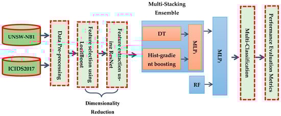
Figure 1. The proposed method.

3.1. Data Description

This study utilizes two established datasets, UNSW-NB15 and CICIDS2017, which will be explained in the subsequent subsections.

3.1.1. UNSW-NB15 Dataset (D1)

The UNSW-NB15 dataset (D1), developed by the Australian Cyber Security Centre [46], is divided into separate training and testing sections. There are 175,341 records in the training set and 83,332 records in the test set. Records in D1 are categorized into two main groups: normal network traffic and different categories of cyberattacks. D1 consists of 44 features, along with two class labels: the attack category and label. In the D1 dataset, there are ten classes in total: one represents normal traffic, while the other nine correspond to various attack types, including Exploits, Worms, Analysis, Fuzzers, Backdoors, Reconnaissance, Generic, DoS, and Shellcode. The class distribution is presented in detail in Table 2.

Table 2. The class distribution in the UNSW-NB15 dataset [47].

Category of Attack	Instance for Training	Instance for Testing
Fuzzers	18,184	6062
Generic	40,000	18,871
Reconnaissance	10,491	3496
Analysis	2000	667
Exploits	33,393	11,132
Backdoor	1746	583
Worms	130	44
Denial of Service (DoS)	12,264	4089
Shellcode	1133	378
Normal traffic	56,000	37,000
Overall total (instances)	175,341	82,332

In dataset D1, the ‘Worms’ class, which contains 174 records, constitutes the minority class, while the ‘Normal’ class, with 93,000 records, represents the majority class. Equation (1) outlines the formula used to calculate these imbalance ratios.

$$\mathrm{Imbalance} \mathrm{Ratio}={\displaystyle \frac{\mathit{C}\mathit{o}\mathit{u}\mathit{n}\mathit{t} \mathit{o}\mathit{f} \mathit{i}\mathit{n}\mathit{s}\mathit{t}\mathit{a}\mathit{n}\mathit{c}\mathit{e}\mathit{s} \mathit{i}\mathit{n} \mathit{m}\mathit{a}\mathit{j}\mathit{o}\mathit{r}\mathit{i}\mathit{t}\mathit{y} \mathit{c}\mathit{l}\mathit{a}\mathit{s}\mathit{s}}{\mathit{C}\mathit{o}\mathit{u}\mathit{n}\mathit{t} \mathit{o}\mathit{f} \mathit{i}\mathit{n}\mathit{s}\mathit{t}\mathit{a}\mathit{n}\mathit{c}\mathit{e} \mathit{i}\mathit{n} \mathit{m}\mathit{i}\mathit{n}\mathit{o}\mathit{r}\mathit{i}\mathit{t}\mathit{y} \mathit{c}\mathit{l}\mathit{a}\mathit{s}\mathit{s}}}$$

(1)

As illustrated in Figure 2, dataset D1 exhibits a significant imbalance. Specifically, the ‘Worms’ class is outnumbered by the ‘Normal’ class, which appears more than 534 times as frequently.

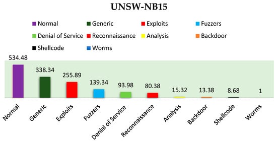
Figure 2. Imbalance ratio of categories in D1.

3.1.2. CICIDS2017 Dataset (D2)

The CICIDS2017 dataset (D2), produced by the Canadian Institute for Cybersecurity (CIC) [48] in 2017, consists of 2,830,743 instances distributed over eight distinct files. Each instance contains 78 attributes along with a label. The D2 dataset comprises 15 classes, including normal traffic and 14 categories of attacks: Web Attack—XSS; Web Attack—SQL Injection; Web Attack—Brute Force; DDoS; FTP—Patator; DoS Hulk; DoS Slowhttptest; DoS slowloris; DoS GoldenEye; Heartbleed; Bot; SSH—Patator; PortScan; and Infiltration. The class distribution of D2 is summarized in Table 3.

Table 3. The class distribution in the CICIDS2017 dataset [48].

Attack Type	Record Count
Normal	2,273,097
PortScan	158,930
Bot	1966
DoS GoldenEye	10,293
SSH—Patator	5897
Web Attack—SQL Injection	21
DoS Slowhttptest	5499
DDoS	128,027
Infiltration	36
FTP—Patator	7938
Web Attack—Brute Force	1507
Heartbleed	11
DoS Hulk	231,073
Web Attack—XSS	652
DoS slowloris	5796
Total attacks	471,454
Overall total (records)	2,830,743

In dataset D2, ‘Heartbleed’ is the minority class with 11 records, while ‘Benign’ is the majority class with 2,273,097 records. Figure 3 illustrates the imbalance ratio across all classes in the D2 dataset, highlighting the substantial class imbalance present. Specifically, the ‘Benign’ class appears more than 206,649 times as often as the ‘Heartbleed’ class.

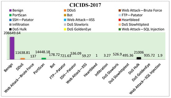
Figure 3. Imbalance ratio of categories in D2.

Utilizing methodologies established by leading authorities on statistical analysis and deep learning [49], we merged the training and testing datasets for both D1 and D2. Afterward, we divided the merged dataset into two distinct, non-overlapping subsets, allocating 80% for training the model and reserving 20% for testing and validation. This approach is particularly suitable for larger datasets, as it avoids the computationally intensive runtime required by k-fold cross-validation. Additionally, it guarantees that the model has enough data for training while still preserving sufficient data for validation and testing. After constructing our model with the training datasets, the subsequent step is to assess its performance in multiclass classification on both D1 and D2.

3.2. Data Pre-Processing

Data pre-processing plays a fundamental role in the data mining process, as it transforms raw data into a format suitable for analysis and knowledge discovery. This step typically consists of three main stages: data filtration, numeralization, and normalization.

3.2.1. Data Filtration

Data from heterogeneous platforms in real-world environments often contain incomplete and inconsistent values, which can significantly affect the effectiveness of machine learning classifiers. In the D2 dataset, the ‘Flow Packets/s’ feature includes abnormal values like ‘NaN’ and ‘Infinity’, which can adversely affect the classification accuracy of predictive models. To address these issues, we implemented basic data cleaning procedures, including the removal of infinite values and incomplete samples from the datasets.

3.2.2. Data Numeralization

This stage transforms symbolic (non-numeric) data into numerical form by applying 1-N numeric coding, where N corresponds to the number of distinct symbols. In this study, all non-numeric data, including ‘state’, ‘proto’, and ‘service’ in D1, were converted into numeric values.

3.2.3. Data Normalization

Min-max normalization plays a vital role in data pre-processing to ensure that features are scaled within a consistent range, typically [0, 1]. Min-max normalization can be represented by the following formula:

$$X_{normalized}={\displaystyle \frac{{X-X}_{min}}{X_{max}-X_{min}}}$$

(2)

where ${\mathit{X}}_{\mathit{n}\mathit{o}\mathit{r}\mathit{m}\mathit{a}\mathit{l}\mathit{i}\mathit{z}\mathit{e}\mathit{d}}$ indicates the value after normalization, and $\mathit{X}$ represents the value before normalization, while ${\mathit{X}}_{\mathit{m}\mathit{i}\mathit{n}}$ and ${\mathit{X}}_{\mathit{m}\mathit{a}\mathit{x}}$ correspond to the minimum and maximum values of the feature, respectively.

3.3. Dimensionality Reduction

Dimensionality refers to the quantity of features included in the dataset [50]. Dimensionality reduction is crucial for converting high-dimensional data into a more manageable low-dimensional representation [51,52]. It has become indispensable in many domains, as its primary goal is to eliminate unimportant, redundant, and noisy features from the dataset, thereby reducing memory requirements [50] and computational complexity [53]. Algorithms that struggle with high dimensionality can benefit significantly from this process, improving their efficiency and accuracy [50]. Dimensionality reduction methods are commonly categorized into two main types: feature selection and feature extraction.

3.3.1. Feature Selection

Feature selection is crucial for the development of an effective IDS [54]. It simplifies datasets by removing redundant and unnecessary features, thereby enhancing the performance of machine learning algorithms [55]. This process helps reduce the training time required for the model while simultaneously enhancing classification accuracy and mitigating overfitting [56].

In our study, we employed an embedded feature selection method using the SelectFromModel (SFM) function from the Scikit-learn package. SFM acts as a meta-transformer that applies importance weights to select features according to a specified threshold, which we set to the mean for this experiment. Specifically, we utilized SFM based on the LogitBoost algorithm [57] to identify important features. LogitBoost was chosen for its ability to handle noisy and outlier data effectively [58], address overfitting issues [59], and manage multiclass problems using multiclass logistic loss [60]. It also reduces training errors and improves generalization capabilities [57]. Notably, LogitBoost requires a regression algorithm as its base estimator, for which we used XGBRegressor [61] in our implementation.

Using LogitBoost, we identified 28 important features from D1 and 35 from D2. Table 4 presents the selected features from both datasets. Algorithm 1 outlines the pre-processing steps integrated with feature selection in our methodology.

Algorithm 1. Pre-processing and Feature Selection Steps

Input: UNSW-NB15 dataset ($D_1$), CICIDS2017 dataset ($D_2$)

Output: Optimal feature subsets chosen by $Z_{LogitBoost -best}$ for $D_1$ and $D_2$

Data Pre-processing // Filtration: Step1:            $D_{pre-pro2}$= Eliminate ‘Infinity’ and ‘NaN’ from $D_2$. // Numeralization: Step2:             If the dataset contains any non-numeric attributes then do:               $D_{pre-pro1}$= used $1-N$ numeric coding to the dataset $D_{pre-pro1}$             End if // Normalization: Step3:               $D_{pre-pro1}$, $D_{pre-pro2}$= applied Min-MaxScaling for ($D_{pre-pro1}$, $D_{pre-pro2}$) // LogitBoost Method Step4: $Z_{LogitBoost -best}$= applied the $\mathrm{L}\mathrm{o}\mathrm{g}\mathrm{i}\mathrm{t}\mathrm{B}\mathrm{o}\mathrm{o}\mathrm{s}\mathrm{t}$ approach based on XGBRegressor for $D_{pre-pro1}$ and $D_{pre-pro2}$          to determine the optimal set of features.

Table 4. Feature selected using LogitBoost method.

Dataset	Feature Count	LogitBoost-Selected Features
D1	28	Dur, service, ct_src_dport_ltm, dmean, ct_srv_src, dpkts, sbytes, ct_dst_src_ltm, sinpkt, dinpkt, ct_dst_ltm, smean, rate, sttl, sload, ct_dst_sport_ltm, dbytes, dtcpb, djit, stcpb, dload, dloss, tcprtt, synack, ackdat, sjit, ct_src_ltm, ct_srv_dst.
D2	35	Destination Port, Flow IAT Min, Flow IAT Max, Total Fwd Packets, Flow Duration, Flow Bytes/s, Fwd Packet Length Std, Flow IAT Std, Fwd Packet Length Mean, Flow IAT Mean, Bwd Packet Length Min, Fwd Packet Length Max, Flow Packets/s, Bwd Packet Length Std, Fwd Packets/s, Fwd IAT Std, Bwd IAT Min, Fwd IAT Mean, Bwd IAT Mean, Fwd IAT Total, Bwd IAT Max, Fwd IAT Min, Bwd IAT Std, Bwd IAT Total, Fwd IAT Max, min_seg_size_forward, Max Packet Length, Init_Win_bytes_forward, Min Packet Length, Init_Win_bytes_backward, Bwd Packets/s, Average Packet Size, PSH Flag Count, Packet Length Std, URG Flag Count.

3.3.2. Feature Extraction

Features extraction [62] involves creating new features from existing ones, offering a valuable method to reduce resource requirements without sacrificing initial feature information. Convolutional Neural Networks (CNNs) are widely used in the field of deep learning for feature extraction. However, they often face challenges such as vanishing and exploding gradients, which the Residual Network (ResNet) architecture addresses [21]. ResNet introduces skip connections, allowing the direct addition of the input from one layer to the output of another. This approach enables the network to learn residual information, significantly enhancing performance and training efficiency. Implementing ResNet architecture not only improves model efficacy but also mitigates issues related to gradient vanishing in Deep Neural Networks.

In this paper, we employed ResNet to extract features selected by the LogitBoost algorithm from D1 and D2. Our ResNet architecture comprises a convolution block, six residual blocks, and global average pooling (GAP), illustrated in Figure 4. The convolution block consists of a convolutional layer, batch normalization (BN), swish activation, and a max pooling layer. The convolutional layer uses kernels to capture diverse features, BN regularizes and accelerates training, and swish is an activation function introduced by Ramachandran et al. [63]. The structure of the residual block includes a convolution layer, batch normalization, swish activation, and a shortcut connection, as depicted in Figure 5. Each unit in the residual block and convolutional block functions identically, except for the shortcut connection, which adds the input of the block to its output.

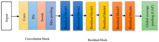
Figure 4. Structure of ResNet.

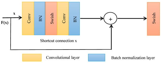
Figure 5. Structure of the residual block.

As illustrated in Figure 5, $\mathit{x}$ stands for the input to the residual block; $\mathit{F}\left(\mathit{x}\right)$ represent the output prior to the second activation function; and F(x) + x denotes the result produced by the residual block with the shortcut connection.

Global average pooling (GAP) is applied to average each feature map. Table 5 displays the parameters associated with the ResNet model.

Table 5. The overall structure and the parameters of the ResNet model.

Layer	Parameters
Convolution layer	Size kernel = 7, number of kernel = 64, stride = 1
Max pooling	Pooling size = 3, stride = 1
Residual block1	Size kernel = 3, number of kernel = 64, stride = 1
Residual block2	Size kernel = 3, number of kernel = 64, stride = 1
Residual block3	Size kernel = 3, number of kernel = 32, stride = 1
Residual block4	Size kernel = 3, number of kernel = 32, stride = 1
Residual block5	Size kernel = 3, number of kernel = 16, stride = 1
Residual block6	Size kernel = 3, number of kernel = 16, stride =1

3.4. Ensemble Learning Classifiers

Ensemble learning classifiers combine multiple algorithms to achieve superior performance compared to individual algorithms. These methodologies are generally categorized into three main types: bagging, boosting, and stacking. Bagging, pioneered by Breiman in 1996 [64], involves training models independently on random subsets of the data and subsequently merging their predictions using a voting process. Boosting, first discussed by Schapire in 1990 [65], builds a model using a sequence of weak classifiers, each one refining the errors identified by its predecessor.

In 1992, Wolpert introduced stacking, commonly referred to as stacked generalization [66]. This approach is recognized for its effectiveness, as it provides a structured approach to combining diverse ensemble algorithms. Stacking operates with two levels of learning: at level 0, base learners are trained on the dataset, generating a new dataset that is used to train a meta-learner at level 1. The meta-learner, which is trained on the predictions made by the base learners, is then utilized to assess the test set.

Although bagging and boosting have significantly contributed to addressing the issues of bias and variance, they do have inherent limitations. Boosting has the potential for overfitting, while bagging suffers from limited diversity among its base models. In contrast, stacking ensemble learning overcomes these drawbacks and offers several benefits:

• Improved accuracy: Stacked ensembles outperform individual predictive models and other ensemble methodologies such as boosting and bagging due to their integration of a diverse range of base models. This comprehensive technique allows for a rigorous analysis of the data, effectively reducing both bias and variance, thereby enhancing predictive accuracy [66].
• Enhanced robustness: Stacked ensembles mitigate overfitting risks and strengthen model robustness by employing a meta-learner to combine base model outputs. This meta-learner is capable of detecting and rectifying the errors of the base models, which leads to improved generalization [67].
• Flexibility: Contrary to boosting and bagging, which generally employ homogeneous model types, stacking ensembles distinguish themselves by integrating various models, comprising both nonlinear and linear ones. This attribute enhances the adaptability of model selection, thereby improving performance when dealing with complex datasets [68].

To capitalize on the benefits of stacking ensemble learning, we propose a novel approach termed multi-stacking ensemble (MSE), aimed at enhancing the performance of multiclass classification for cybersecurity threats. The MSE utilizes a two-level structure comprising various base models, comprising both nonlinear and linear approaches. This design enables the MSE to capture various facets of the data, effectively reducing bias and variance, thereby enhancing performance on complex datasets. Additionally, the MSE incorporates two meta-learners, which serve to mitigate overfitting and strengthen the model’s robustness. These meta-learners are capable of identifying and correcting the errors produced by the base models, ultimately improving the overall generalization performance.

3.4.1. Decision Tree Classifier

Decision tree (DT) remains a robust and commonly utilized data mining technique, playing critical roles in decision-making and classification processes [69]. Its operational efficacy persists even in scenarios with a large number of attributes and substantial datasets, as the tree’s size remains unaffected by the dataset’s extent [70]. Decision trees are distinguished by their quick training and processing speeds, making them apt for handling large datasets [71].

3.4.2. Histogram-Based Gradient Boosting Classifier

Also known as ‘hist-based gradient boosting’ [72], this boosting ensemble algorithm utilizes feature histograms for the rapid and precise selection of optimal splits. It demonstrates significant efficacy when applied to large datasets [73], optimizing computational efficiency by reducing processing duration while maintaining accuracy and minimizing memory utilization [74].

3.4.3. Random Forest Classifier

Breiman’s random forest (RF) [75], a classification method based on ensemble learning, generates multiple decision trees using bootstrap samples derived from the original dataset. RF is distinguished by several key advantages: it predicts important variables, reduces classification errors, handles imbalanced datasets efficiently, manages large datasets with numerous variables, mitigates the risk of overfitting, and maintains classification accuracy across different datasets. These benefits establish RF as a reliable and adaptable method for classification tasks.

3.4.4. Multilayer Perceptron Algorithm

The Multilayer Perceptron (MLP) is a feed-forward neural network with at least three layers: an input layer, one or more hidden layer, and an output layer. The MLP is trained on a dataset using the backpropagation method to learn the function $f\left(x\right):R^m\to R^o$. In this context, $m$ denotes the input dimensions, and $o$ indicates the output dimensions. Each layer in an MLP can be described using the following equivalent equations:

$$y=\varnothing \left({\sum }_{i=1}^n{W}_{i}X+b\right)$$

(3)

$$y=\varnothing (W^{T}X+b)$$

(4)

where $W$ represents the weight vector, $\varnothing$ refers to the activation function, $b$ stands for the bias, and $X$ is the input vector.

3.4.5. Multi-Stacking Ensemble (MSE)

This section introduces our proposed MSE classifier, which consists of three levels of classifiers. The first level includes two base classifiers: decision tree (DT) and histogram-based gradient boosting. From the initial dataset, this level trains the data independently and introduces the obtained predictions to the next level (i.e., MLP₁). However, the second level incorporates a meta-classifier, MLP₁, along with an additional base classifier (i.e., RF). The MLP₁ will train the data obtained from level one, while the RF will train the data produced from ResNet. Then, the obtained predictions introduced from the second level will be provided to the third level (i.e., MLP₂). Finally, the third level, which includes another meta-classifier (MLP₂), trains the predictions resulting from level two and generates the final enhanced prediction.

The training dataset (D) for the base classifiers is constructed using features extracted by ResNet. To mitigate overfitting during training, we employ a k-fold cross-validation technique. In this approach, the training data (D) are split into K distinct, equally sized subsets ($D_{t1}, D_{t2},D_{t3},{\dots ,D}_{tn}$). One subset is reserved for testing, while the remaining $k-1/k$ subsets are used to train the classifiers.

In this study, the MSE employs two meta-learners. The input for the first meta-learner (MLP₁) includes DT and hist-gradient boosting algorithms as base classifiers, while the input for the second meta-learner (MLP₂) includes the output of MLP₁ and the base classifier of the RF algorithm. The parameters for the MSE are presented in Table 6, and Algorithm 2 outlines the general workflow of the MSE.

Algorithm 2. Multi-Stacking Ensemble

Input: Train data $D$ = ${\left\{x_i,y_i\right\}}_{\left(i=1\right)}; \left(x_iϵR^n, y_iϵ y\right)$, where $x_i$ represents features and $y_i$ represents the label.

Output: the final predictions output (F)

// Prepare training set using cross-validation Step 1: Apply five-fold cross-validation in preparing the training set.  // Splitting the dataset into five equally sized subsets. Step 2: Randomly Split $D$ into $K=5$ equally sized subsets.  Step 3: for $k\leftarrow 1 to KF$  do      where $KF=5$           Step 3.1: for $kk\leftarrow 1 to K$  do      where $K=5$                           Employ base level classifiers (DT, hist-gradient boosting)                               for $t\leftarrow 1 to T$do                                Learn a classifier $h_{kkt}$ from $DKF\backslash D_{KK}$                               end for                            Construct a training set for first meta-classifier (${ml}_1$) MLP1                                 for $x_i\in D_{KK}$ do                                 Get record {${\acute{x}}_i,y_i$}, where ${\acute{x}}_i=\left\{h_{kk1}\left(x_i\right),h_{kk2}\left(x_i\right), \dots , h_{kkT}\left(x_i\right)\right\}$                                 end for                      end for             Step 3.2: Learn the first meta-classifier (${ml}_1$) MLP1                    Learn a new classifier $\acute{h}$ from the collection of { ${\acute{x}}_i,y_i\}$               Step 3.3: Re-learn classifiers                        for $t\leftarrow 1 to T$do                           Learn a classifier ${(h}_t)$ based on $DKF$                          end for              Step 3.4: $H\left(x\right)=\acute{h}\left(h_1\left(x\right),h_2\left(x\right), \dots , h_T\left(x\right)\right)$             Step 3.5: Employ base level classifiers ($H\left(x\right)$, RF)                              for $t\leftarrow 1 to T$do                             Learn a classifier $f_{KFt}$ from $D\backslash D_{KF}$                            end for                         Construct a training set for the second meta classifier (${ml}_2$) MLP2                            for $z_i\in D_{KF}$ do                             Get record {${\acute{z}}_i,m_i$}, where ${\acute{z}}_i=\left\{f_{KF1}\left(z_i\right),f_{KF2}\left(z_i\right), \dots , f_{KFT}\left(z_i\right)\right\}$                            end for         end for Step 4: Learn the second meta-classifier (${ml}_2$) MLP2         Learn a new classifier $\acute{f}$ from the collection of { $z_i,m_i\}$ Step 5: Re-learn classifiers          for $t\leftarrow 1 to T$do            Learn a classifier ${(f}_t)$ based on $\mathrm{D}$         end for Step 6: Return $F\left(x\right)=\acute{f}\left(f_1\left(z\right),f_2\left(z\right), \dots , f_t\left(z\right)\right)$

Table 6. Experimental model parameters.

Algorithms	Parameters
DT	Criterion = ‘entropy’, min_samples_leaf = 5, min_samples_split = 2.
Hist-gradient boosting	Loss = ‘categorical_crossentropy’, min_samples_leaf = 10, learning_rate = 0.1.
RF	N_estimators = 100, criterion = ‘entropy’, max_depth = 60.
MLP	Hidden_layer_sizes with 100 neurons, activation = ‘relu’, solver = ‘adam’.

4. Performance Evaluation

In this section, we assess the performance of our proposed model by applying various prominent and widely recognized metrics, including accuracy, F1 score, recall, and precision [13]. These evaluation metrics are calculated from the confusion matrix, which is built upon the following four values:

• False positive (FP): the actual data are negative, but the prediction indicates them as positive.
• False negative (FN): the actual data are positive, but the prediction incorrectly indicates them as negative.
• True negative (TN): both the actual data and the prediction are negative.
• True positive (TP): both the actual data and the prediction are positive.

Accuracy is a measure of the model’s performance, calculated as the ratio of correctly classified instances to the total number of instances in the dataset. It is calculated using the following formula:

$$Accuracy={\displaystyle \frac{TP+TN}{TP+TN+FP+FN}}$$

(5)

Recall is the ratio of correctly identified positive cases (TP) to the total number of true positive (TP) and false negative (FN) cases. This can be described as follows:

$$Recall={\displaystyle \frac{TP}{TP+FN}}$$

(6)

Precision represents the proportion of correctly predicted positives (TPs) out of all cases that were predicted as positive, which includes both true positives (TPs) and false positives (FPs). It is calculated using the following formula:

$$Precision={\displaystyle \frac{TP}{TP+FP}}$$

(7)

The F1 score represents the harmonic mean of precision and recall. It is expressed as follows:

$$F_1 \mathrm{score}=2\times \left({\displaystyle \frac{Precision\times Recall}{Precision+Recall}}\right)$$

(8)

4.1. Experimental Results and Discussion

In this section, we focus on analyzing the performance of the proposed MSE classifier by benchmarking it against a variety of individual algorithms, as well as comparing it with state-of-the-art methods. The model was evaluated using Python within the Jupyter Notebook environment. In our experiments, we used such libraries as Scikit-learn, Pandas, and NumPy. Scikit-learn is an efficient machine learning and data modeling tool utilized for the purpose of data analysis, whereas NumPy and Pandas are machine learning and deep learning libraries dealing with data structure management, data manipulation and analysis, and computational processing [76]. Our experiments were conducted on a system with the following hardware and software specifications:

• Windows 11 (64-bit) as the operating system.
• VGA: RTX2070 8GB.
• HDD: 1 TB SSD.
• RAM: 32 GB.
• CPU: Ryzen7 5800h.

4.2. Comparing Individual Algorithms with MSE for Multiclass Classification

In our evaluation, we rigorously tested the MSE classifier’s performance against several individual classification algorithms, including DT, hist-gradient boosting, RF, and MLP. These assessments utilized the LogitBoost and ResNet algorithms within a multiclassification framework, focusing on the D1 dataset. The results are summarized in Table 7.

Table 7. Evaluation of multiclass classification results for D1.

Classifier	Category of Attack	Precision	Recall	F1 Score
DT	Analysis	66.66	10.09	17.53
	Backdoor	50.81	6.65	11.76
	DoS	43.90	17.05	24.57
	Exploits	61.59	89.10	72.84
	Fuzzers	71.52	53.51	61.22
	Generic	99.17	97.76	98.46
	Normal	90.32	94.05	92.15
	Reconnaissance	89.25	74.51	81.22
	Shellcode	54.16	51.65	52.88
	Worms	33.33	11.42	17.02
Hist-gradient boosting	Analysis	74.68	11.02	19.21
	Backdoor	52.27	4.93	9.01
	DoS	45.62	11.46	18.32
	Exploits	61.12	91.04	73.14
	Fuzzers	75.71	55.31	63.92
	Generic	99.40	98.03	98.71
	Normal	90.64	95.08	92.81
	Reconnaissance	90.50	73.90	81.36
	Shellcode	53.82	58.27	55.96
	Worms	16.66	22.85	19.27
RF	Analysis	69.56	11.96	20.41
	Backdoor	64	6.86	12.40
	DoS	34.06	23.23	27.62
	Exploits	63.41	82.63	71.76
	Fuzzers	70.92	59.31	64.60
	Generic	99.63	97.92	98.77
	Normal	91.64	94.98	93.28
	Reconnaissance	89.96	75.91	82.34
	Shellcode	63.95	59.93	61.88
	Worms	33.33	8.50	13.63
MLP	Analysis	65.16	10.84	18.58
	Backdoor	57.62	7.29	12.95
	DoS	44.25	25.31	32.20
	Exploits	63.79	88.26	74.06
	Fuzzers	73.54	59.22	65.61
	Generic	99.44	98.06	98.74
	Normal	91.75	94.15	92.93
	Reconnaissance	91.35	75.12	82.44
	Shellcode	64.94	58.27	61.43
	Worms	27.27	17.14	21.05
Proposed model (MSE)	Analysis	81.14	26.54	40
	Backdoor	72.80	17.81	28.62
	DoS	59.64	49.25	53.95
	Exploits	73.74	90.06	81.08
	Fuzzers	89.32	84.36	86.77
	Generic	99.82	99.06	99.44
	Normal	98.19	98.37	98.28
	Reconnaissance	95.93	82.70	88.82
	Shellcode	87.22	92.71	89.88
	Worms	76.92	85.71	81.08

Individual classifiers exhibited varying success rates in identifying different attack classes. The DT, hist-gradient boosting, RF, and MLP algorithms showed suboptimal performance in detecting Analysis, Backdoor, DoS, and Worm attacks. In particular, the MLP demonstrated better capability in identifying DoS and Worm attacks compared to other individual algorithms. In contrast, our MSE model showcased significant improvements across most classes in the D1 dataset, effectively mitigating the limitations observed in individual classifiers, as detailed in Table 7. Figure 6 presents the confusion matrices of MSE for multiclass classification in D1, offering a comprehensive visual representation of the model’s performance.

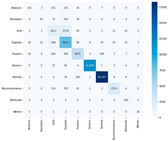
Figure 6. Multiclass confusion matrix for D1.

Table 8 outlines the performance results of the MSE classifier alongside various individual classifiers for the D2 dataset. The DT algorithm encountered challenges in identifying four attacks: Heartbleed; Infiltration; Web Attack—SQL Injection; and Web Attack—XSS. Hist-gradient boosting struggled with three attacks: Heartbleed, Infiltration, and Web Attack—SQL Injection. It also exhibited poor performance for Web Attack—Brute Force—and Web Attack—XSS. RF failed to identify Infiltration and Web Attack—SQL Injection—with particularly low performance for Web Attack—XSS. The MLP also faced difficulties in identifying Infiltration and Web Attack—SQL Injection—but displayed better results for Web Attack—XSS—compared to other individual classifiers.

Table 8. Evaluation of multiclass classification results for D2.

Classifier	Category of Attack	Precision	Recall	F1 Score
DT	Benign	99.54	98.69	99.11
	Bot	91.94	35.03	50.74
	DdoS	99.59	99.68	99.64
	DoS GoldenEye	95.63	95.72	95.67
	DoS Hulk	97.98	99.31	98.64
	DoS Slowhttptest	95.17	98.63	96.87
	DoS slowloris	96.75	95.08	95.90
	FTP—Patator	97.49	97.98	97.73
	Heartbleed	0	0	0
	Infiltration	0	0	0
	PortScan	86.38	96.08	90.98
	SSH—Patator	98.03	92.79	95.34
	Web Attack—Brute Force	64.86	87.70	74.57
	Web Attack—SQL Injection	0	0	0
	Web Attack—XSS	0	0	0
Hist-gradient boosting	Benign	99.54	98.53	99.03
	Bot	44.10	43.98	44.04
	DdoS	99.90	98.76	99.33
	DoS GoldenEye	96.98	85.96	91.14
	DoS Hulk	98.29	99.28	98.78
	DoS Slowhttptest	75.98	98.09	85.63
	DoS slowloris	91.48	96.46	93.91
	FTP—Patator	96.27	97.79	97.03
	Heartbleed	0	0	0
	Infiltration	0	0	0
	PortScan	89.82	95.34	92.50
	SSH—Patator	95.19	95.76	95.47
	Web Attack—Brute Force	22.60	88.70	36.03
	Web Attack—SQL Injection	0	0	0
	Web Attack—XSS	1.04	2.30	1.44
RF	Benign	99.67	98.61	99.14
	Bot	100	37.85	54.91
	DdoS	99.98	99.77	99.88
	DoS GoldenEye	99.21	97.71	98.45
	DoS Hulk	98.56	99.23	98.89
	DoS Slowhttptest	98.28	98.90	98.59
	DoS slowloris	99.71	89.21	94.17
	FTP—Patator	99.60	95.84	97.68
	Heartbleed	100	100	100
	Infiltration	0	0	0
	PortScan	84.79	98.39	91.09
	SSH—Patator	98.82	92.45	95.53
	Web Attack—Brute Force	69.35	97	80.88
	Web Attack—SQL Injection	0	0	0
	Web Attack—XSS	33	0.76	1.50
MLP	Benign	99.56	99.02	99.29
	Bot	89.67	42.19	57.39
	DdoS	99.91	99.73	99.82
	DoS GoldenEye	98.50	99.02	98.76
	DoS Hulk	98.26	99.65	98.95
	DoS Slowhttptest	97.58	99	98.28
	DoS slowloris	99.12	97.75	98.43
	FTP—Patator	97.77	99.55	98.65
	Heartbleed	100	100	100
	Infiltration	0	0	0
	PortScan	89.67	95.81	92.64
	SSH—Patator	98.10	96.35	97.22
	Web Attack—Brute Force	65.11	55.81	60.10
	Web Attack—SQL Injection	0	0	0
	Web Attack—XSS	26	12	16.84
Proposed model (MSE)	Benign	99.86	99.79	99.83
	Bot	92.92	73.91	82.33
	DdoS	99.98	99.93	99.95
	DoS GoldenEye	99.85	99.46	99.65
	DoS Hulk	99.78	99.93	99.86
	DoS Slowhttptest	99.09	99.09	99.09
	DoS slowloris	99.65	99.82	99.74
	FTP—Patator	99.93	99.87	99.90
	Heartbleed	100	100	100
	Infiltration	100	71.42	83.33
	PortScan	97.48	98.56	98.01
	SSH—Patator	99.40	99.74	99.57
	Web Attack—Brute Force	73.27	81.06	76.97
	Web Attack—SQL Injection	80	100	88.88
	Web Attack—XSS	42.45	34.61	38.13

In contrast, our proposed MSE model demonstrated substantial improvements, effectively identifying most attack classes in the D2 dataset and addressing the limitations observed in individual algorithms, as depicted in Table 8. Figure 7 illustrates the confusion matrices of MSE for multiclass classification in D2, providing a comprehensive visual insight into the model’s performance.

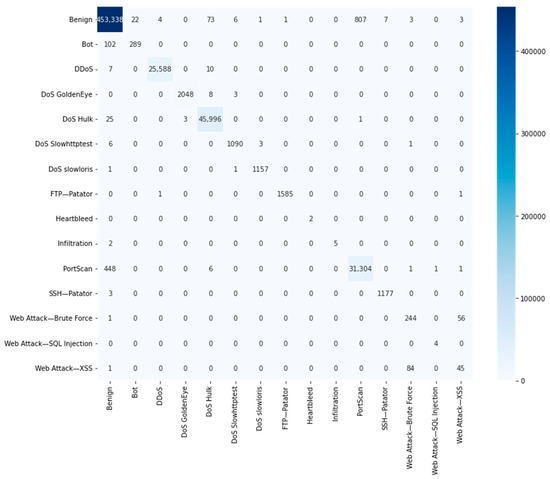
Figure 7. Multiclass confusion matrix for D2.

4.3. Comparison of Results with State-of-the-Art Models

This section provides a comparison between the performance of our proposed model and previous research on multiclass classification, utilizing the D1 and D2 datasets. The evaluation metrics are outlined in Table 9 and Table 10. Table 9 illustrates the multiclass classification results of our model alongside those of recent IDS research for D1, while Table 10 presents the performance for D2.

Table 9. Performance metrics comparison between our proposed model and recent IDS models for multiclass classification on the UNSW-NB15 dataset (bold indicates best results).

Ref.	Dataset	Dimensionality Reduction Techniques	Classification Techniques	Accuracy (%)	Recall (%)	Precision (%)	F1 Score (%)
[77]	D1	IGRF-RFE	MLP	84.24	84.24	83.6	82.85
[78]	D1	N/A	Early-fusion deep learning	76.47	71.59	83.53	N/A
[78]	D1	N/A	Late-fusion deep learning	77.09	69.5	86.04	N/A
[78]	D1	N/A	Late-ensemble deep learning	76.84	68.18	85.92	N/A
[79]	D1	N/A	Deep SARSA	82.62	82.6	82.4	82.49
[80]	D1	CNN	BLSTM	76.32	76	81	77
[81]	D1	NRS-SSA	Adaptive ensemble (DT, KNN, RF, XGBoost)	81.54	81.54	82.7	79.7
[82]	D1	Hierarchical Clustering	DTTWSVM	81.21	N/A	N/A	N/A
[83]	D1	RF-SFS	ANN	78.23	68.85	85.13	76.13
[83]	D1	RF-SFS	GRU	79	63	70	62
[83]	D1	RF-SFS	LSTM	78	63	70	64
[84]	D1	N/A	Ensemble (group convolution network snapshot ensemble)	79.59	80.38	81.27	80.82
[85]	D1	UMAP	RF	81.6	80	N/A	80
This study	D1	LogitBoost-ResNet	MSE	90.29	90.29	90.45	89.87

Table 10. Performance metrics comparison between our proposed model and recent IDS models for multiclass classification on the CICIDS2017 dataset (bold indicates best results).

Ref.	Dataset	Dimensionality Reduction Techniques	Classification Techniques	Accuracy (%)	Recall (%)	Precision (%)	F1 Score (%)
[86]	D2	N/A	Stacking (CNN, DNN, LSTM, MLP)	98.7	98.7	98.7	98.6
[80]	D2	CNN	BLSTM	98	98	99	98
[87]	D2	Greedy-RFECV	Global and local subnet parallel Deep Neural Network (CGL-DNN)	85	N/A	N/A	86
[88]	D2	Chi-squared	Triple-layered hybrid (weighted DNN, CNN+LSTM, XGBoost)	98.46	98.21	86.42	98.1
This study	D2	LogitBoost-ResNet	MSE	99.69	99.69	99.69	99.69

The results in Table 9 underscore the effective overall performance of our proposed model relative to previous studies. For multiclass classification on D1, our model achieves an accuracy of 90.29%, a recall of 90.29%, a precision of 90.45%, and an F1 score of 89.87%. Moving to D2, the multiclass classification accuracy reaches an impressive 99.70%, with the precision, recall, and F1 score all at 99.70%.

5. Conclusions

With the continuous expansion of Internet usage, ensuring robust network security in distributed systems has become increasingly critical. Although numerous machine learning algorithms have been applied in previous research to improve the performance of intrusion detection systems (IDSs), achieving optimal results remains a challenge, particularly when dealing with high-dimensional data. IDSs still face vulnerabilities in classification, such as the risk of single algorithm failure in multiclass attack scenarios. To address these limitations, we propose a novel dimensionality reduction approach that integrates feature selection and feature extraction techniques to enhance the IDS dataset. Additionally, to mitigate issues related to multiclass attack detection, we introduce a new multi-stacking ensemble classifier, which we evaluate using two widely recognized intrusion detection benchmark datasets. Our methodology began with the LogitBoost algorithm to select optimal features from the datasets. Subsequently, we employed the ResNet algorithm to construct new features based on those selected by LogitBoost. Finally, we developed and evaluated a multi-stacking ensemble model.

The experimental results demonstrated outstanding performance in multiclass classification for both datasets. Specifically, our model achieved high metrics on the UNSW-NB15 (D1) dataset: an accuracy of 90.29%, a recall of 90.29%, a precision of 90.45%, and an F1 score of 89.87%. For the CICIDS2017 (D2) dataset, our model achieved an exceptional multiclass classification accuracy of 99.69%, with the corresponding recall, precision, and F1 score also at 99.69%. These results show better performance for our model compared to state-of-the-art methods in the field of intrusion detection.

References

- Leszczyna, R.; Wallis, T.; Wróbel, M.R. Developing novel solutions to realise the European energy–information sharing & analysis centre. Decis. Support Syst. 2019, 122, 113067. [Google Scholar]
- Koczkodaj, W.W.; Mazurek, M.; Strzałka, D.; Wolny-Dominiak, A.; Woodbury-Smith, M. Electronic health record breaches as social indicators. Soc. Indic. Res. 2019, 141, 861–871. [Google Scholar] [CrossRef]
- Zhang, H.; Chari, K.; Agrawal, M. Decision support for the optimal allocation of security controls. Decis. Support Syst. 2018, 115, 92–104. [Google Scholar] [CrossRef]
- Zadeh, A.; Jeyaraj, A. A multistate modeling approach for organizational cybersecurity exploration and exploitation. Decis. Support Syst. 2022, 162, 113849. [Google Scholar] [CrossRef]
- Khammassi, C.; Krichen, S. A GA-LR wrapper approach for feature selection in network intrusion detection. Comput. Secur. 2017, 70, 255–277. [Google Scholar] [CrossRef]
- Yang, B.; Arshad, M.H.; Zhao, Q. Packet-level and flow-level network intrusion detection based on reinforcement learning and adversarial training. Algorithms 2022, 15, 453. [Google Scholar] [CrossRef]
- Elhag, S.; Fernández, A.; Bawakid, A.; Alshomrani, S.; Herrera, F. On the combination of genetic fuzzy systems and pairwise learning for improving detection rates on intrusion detection systems. Expert Syst. Appl. 2015, 42, 193–202. [Google Scholar] [CrossRef]
- Khraisat, A.; Gondal, I.; Vamplew, P.; Kamruzzaman, J. Survey of intrusion detection systems: Techniques, datasets and challenges. Cybersecurity 2019, 2, 1–22. [Google Scholar] [CrossRef]
- Anwar, S.; Mohamad Zain, J.; Zolkipli, M.F.; Inayat, Z.; Khan, S.; Anthony, B.; Chang, V. From intrusion detection to an intrusion response system: Fundamentals, requirements, and future directions. Algorithms 2017, 10, 39. [Google Scholar] [CrossRef]
- Li, X.J.; Ma, M.; Sun, Y. An adaptive deep learning neural network model to enhance machine-learning-based classifiers for intrusion detection in smart grids. Algorithms 2023, 16, 288. [Google Scholar] [CrossRef]
- Wan, J.; Waqas, M.; Tu, S.; Hussain, S.M.; Shah, A.; Rehman, S.U.; Hanif, M. An efficient impersonation attack detection method in fog computing. CMC-Comput. Mater. Cont. 2021, 68, 267–281. [Google Scholar] [CrossRef]
- Pranto, M.B.; Ratul, M.H.A.; Rahman, M.M.; Diya, I.J.; Zahir, Z.-B. Performance of machine learning techniques in anomaly detection with basic feature selection strategy-a network intrusion detection system. J. Adv. Inf. Technol 2022, 13, 36–44. [Google Scholar] [CrossRef]
- Ozkan-Okay, M.; Samet, R.; Aslan, Ö.; Gupta, D. A comprehensive systematic literature review on intrusion detection systems. IEEE Access 2021, 9, 157727–157760. [Google Scholar] [CrossRef]
- Cui, J.; Zong, L.; Xie, J.; Tang, M. A novel multi-module integrated intrusion detection system for high-dimensional imbalanced data. Appl. Intell. 2023, 53, 272–288. [Google Scholar] [CrossRef]
- Kim, M.; Yun, J.; Cho, Y.; Shin, K.; Jang, R.; Bae, H.-j.; Kim, N. Deep learning in medical imaging. Neurospine 2019, 16, 657. [Google Scholar] [CrossRef]
- Yin, W.; Kann, K.; Yu, M.; Schütze, H. Comparative study of CNN and RNN for natural language processing. arXiv 2017, arXiv:1702.01923. [Google Scholar]
- Liu, L.; Wang, P.; Lin, J.; Liu, L. Intrusion detection of imbalanced network traffic based on machine learning and deep learning. IEEE Access 2020, 9, 7550–7563. [Google Scholar] [CrossRef]
- Esteva, A.; Robicquet, A.; Ramsundar, B.; Kuleshov, V.; DePristo, M.; Chou, K.; Cui, C.; Corrado, G.; Thrun, S.; Dean, J. A guide to deep learning in healthcare. Nat. Med. 2019, 25, 24–29. [Google Scholar] [CrossRef]
- Sun, X.; Lv, M. Facial expression recognition based on a hybrid model combining deep and shallow features. Cogn. Comput. 2019, 11, 587–597. [Google Scholar] [CrossRef]
- Chen, C.; Song, Y.; Yue, S.; Xu, X.; Zhou, L.; Lv, Q.; Yang, L. Fcnn-se: An intrusion detection model based on a fusion CNN and stacked ensemble. Appl. Sci. 2022, 12, 8601. [Google Scholar] [CrossRef]
- He, K.; Zhang, X.; Ren, S.; Sun, J. Deep residual learning for image recognition. In Proceedings of the IEEE Conference on Computer Vision and Pattern Recognition, Las Vegas, NV, USA, 27–30 June 2016; pp. 770–778. [Google Scholar]
- Mebawondu, J.O.; Alowolodu, O.D.; Mebawondu, J.O.; Adetunmbi, A.O. Network intrusion detection system using supervised learning paradigm. Sci. Afr. 2020, 9, e00497. [Google Scholar] [CrossRef]
- Zhang, L.; Xu, C. A Intrusion Detection Model Based on Convolutional Neural Network and Feature Selection. In Proceedings of the 2022 5th International Conference on Artificial Intelligence and Big Data (ICAIBD), Chengdu, China, 27–30 May 2022; pp. 162–167. [Google Scholar]
- Alazzam, H.; Sharieh, A.; Sabri, K.E. A feature selection algorithm for intrusion detection system based on pigeon inspired optimizer. Expert Syst. Appl. 2020, 148, 113249. [Google Scholar] [CrossRef]
- Tang, C.; Luktarhan, N.; Zhao, Y. An efficient intrusion detection method based on LightGBM and autoencoder. Symmetry 2020, 12, 1458. [Google Scholar] [CrossRef]
- Wang, Z.; Liu, J.; Sun, L. EFS-DNN: An Ensemble Feature Selection-Based Deep Learning Approach to Network Intrusion Detection System. Secur. Commun. Netw. 2022, 2022, 2693948. [Google Scholar] [CrossRef]
- Chowdhury, R.; Sen, S.; Roy, A.; Saha, B. An optimal feature based network intrusion detection system using bagging ensemble method for real-time traffic analysis. Multimed. Tools Appl. 2022, 81, 41225–41247. [Google Scholar] [CrossRef]
- Kannari, P.R.; Chowdary, N.S.; Biradar, R.L. An anomaly-based intrusion detection system using recursive feature elimination technique for improved attack detection. Theor. Comput. Sci. 2022, 931, 56–64. [Google Scholar] [CrossRef]
- Nazir, A.; Khan, R.A. A novel combinatorial optimization based feature selection method for network intrusion detection. Comput. Secur. 2021, 102, 102164. [Google Scholar] [CrossRef]
- Jiang, H.; He, Z.; Ye, G.; Zhang, H. Network intrusion detection based on PSO-XGBoost model. IEEE Access 2020, 8, 58392–58401. [Google Scholar] [CrossRef]
- Zong, X.; Li, R.; Ye, Z. An Intrusion Detection Model Based on Improved Whale Optimization Algorithm and XGBoost. In Proceedings of the 2021 11th IEEE International Conference on Intelligent Data Acquisition and Advanced Computing Systems: Technology and Applications (IDAACS), Virtual, 22–25 September 2021; pp. 542–547. [Google Scholar]
- Yong, X.; Gao, Y. Hybrid firefly and black hole algorithm designed for XGBoost tuning problem: An application for intrusion detection. IEEE Access 2023, 11, 28551–28564. [Google Scholar] [CrossRef]
- Iwendi, C.; Khan, S.; Anajemba, J.H.; Mittal, M.; Alenezi, M.; Alazab, M. The use of ensemble models for multiple class and binary class classification for improving intrusion detection systems. Sensors 2020, 20, 2559. [Google Scholar] [CrossRef]
- Zheng, X.; Wang, Y.; Jia, L.; Xiong, D.; Qiang, J. Network intrusion detection model based on Chi-square test and stacking approach. In Proceedings of the 2020 7th International Conference on Information Science and Control Engineering (ICISCE), Changsha, China, 18–20 December 2020; pp. 894–899. [Google Scholar]
- Rajadurai, H.; Gandhi, U.D. A stacked ensemble learning model for intrusion detection in wireless network. Neural Comput. Appl. 2022, 34, 15387–15395. [Google Scholar] [CrossRef]
- Jain, M.; Kaur, G. Distributed anomaly detection using concept drift detection based hybrid ensemble techniques in streamed network data. Clust. Comput. 2021, 24, 2099–2114. [Google Scholar] [CrossRef]
- Alsaffar, A.M.; Nouri-Baygi, M.; Zolbanin, H.M. Shielding networks: Enhancing intrusion detection with hybrid feature selection and stack ensemble learning. J. Big Data 2024, 11, 133. [Google Scholar] [CrossRef]
- Luo, J.; Zhang, Y.; Wu, Y.; Xu, Y.; Guo, X.; Shang, B. A multi-channel contrastive learning network based intrusion detection method. Electronics 2023, 12, 949. [Google Scholar] [CrossRef]
- Sherubha, P.; Sasirekha, S.; Anguraj, A.D.K.; Rani, J.V.; Anitha, R.; Praveen, S.P.; Krishnan, R.H. An Efficient Unsupervised Learning Approach for Detecting Anomaly in Cloud. Comput. Syst. Sci. Eng. 2023, 45, 149–166. [Google Scholar] [CrossRef]
- Yan, Y.; Qi, L.; Wang, J.; Lin, Y.; Chen, L. A network intrusion detection method based on stacked autoencoder and LSTM. In Proceedings of the ICC 2020-2020 IEEE International Conference on Communications (ICC), Dublin, Ireland, 7–11 June 2020; pp. 1–6. [Google Scholar]
- Du, X.; Lin, L.; Han, Z.; Zhang, C. An Intrusion Detection Algorithm Based on Hybrid Autoencoder and Decision Tree. In Proceedings of the 2022 12th International Conference on Information Science and Technology (ICIST), Kaifeng, China, 14–16 October 2022; pp. 32–37. [Google Scholar]
- Singh, S. Poly logarithmic naive Bayes intrusion detection system using linear stable PCA feature extraction. Wirel. Pers. Commun. 2022, 125, 3117–3132. [Google Scholar] [CrossRef]
- Waskle, S.; Parashar, L.; Singh, U. Intrusion detection system using PCA with random forest approach. In Proceedings of the 2020 International Conference on Electronics and Sustainable Communication Systems (ICESC), Coimbatore, India, 2–4 July 2020; pp. 803–808. [Google Scholar]
- Karanam, L.; Pattanaik, K.K.; Aldmour, R. Intrusion detection mechanism for large scale networks using CNN-LSTM. In Proceedings of the 2020 13th International Conference on Developments in eSystems Engineering (DeSE), Liverpool, UK, 14–17 December 2020; pp. 323–328. [Google Scholar]
- Zhao, Z.; Ge, L.; Zhang, G. A novel DBN-LSSVM ensemble method for intrusion detection system. In Proceedings of the 2021 9th International Conference on Communications and Broadband Networking, Shanghai, China, 25–27 February 2021; pp. 101–107. [Google Scholar]
- Moustafa, N.; Slay, J. UNSW-NB15: A comprehensive data set for network intrusion detection systems (UNSW-NB15 network data set). In Proceedings of the 2015 Military Communications and Information Systems Conference (MilCIS), Canberra, Australia, 10–12 November 2015; pp. 1–6. [Google Scholar]
- Awad, M.; Fraihat, S. Recursive feature elimination with cross-validation with decision tree: Feature selection method for machine learning-based intrusion detection systems. J. Sens. Actuator Netw. 2023, 12, 67. [Google Scholar] [CrossRef]
- Sharafaldin, I.; Lashkari, A.H.; Ghorbani, A.A. Toward generating a new intrusion detection dataset and intrusion traffic characterization. ICISSp 2018, 1, 108–116. [Google Scholar]
- Hastie, T.; Tibshirani, R.; Friedman, J.H.; Friedman, J.H. The Elements of Statistical Learning: Data Mining, Inference, and Prediction; Springer: Berlin/Heidelberg, Germany, 2009; Volume 2. [Google Scholar]
- Velliangiri, S.; Alagumuthukrishnan, S. A review of dimensionality reduction techniques for efficient computation. Procedia Comput. Sci. 2019, 165, 104–111. [Google Scholar] [CrossRef]
- Santos, I.; Young, A. Exploring the perception of social characteristics in faces using the isolation effect. Vis. Cogn. 2005, 12, 213–247. [Google Scholar] [CrossRef]
- Chao, G.; Luo, Y.; Ding, W. Recent advances in supervised dimension reduction: A survey. Mach. Learn. Knowl. Extr. 2019, 1, 341–358. [Google Scholar] [CrossRef]
- Ayesha, S.; Hanif, M.K.; Talib, R. Overview and comparative study of dimensionality reduction techniques for high dimensional data. Inf. Fusion 2020, 59, 44–58. [Google Scholar] [CrossRef]
- Zhou, Y.; Ren, H.; Li, Z.; Pedrycz, W. Anomaly detection based on a granular Markov model. Expert Syst. Appl. 2022, 187, 115744. [Google Scholar] [CrossRef]
- Alkanhel, R.; El-kenawy, E.-S.M.; Abdelhamid, A.A.; Ibrahim, A.; Alohali, M.A.; Abotaleb, M.; Khafaga, D.S. Network Intrusion Detection Based on Feature Selection and Hybrid Metaheuristic Optimization. Comput. Mater. Contin. 2023, 74. [Google Scholar] [CrossRef]
- Naseri, T.S.; Gharehchopogh, F.S. A feature selection based on the farmland fertility algorithm for improved intrusion detection systems. J. Netw. Syst. Manag. 2022, 30, 40. [Google Scholar] [CrossRef]
- Friedman, J.; Hastie, T.; Tibshirani, R. Additive logistic regression: A statistical view of boosting (with discussion and a rejoinder by the authors). Ann. Stat. 2000, 28, 337–407. [Google Scholar] [CrossRef]
- Hall, M.; Frank, E.; Holmes, G.; Pfahringer, B.; Reutemann, P.; Witten, I.H. The WEKA data mining software: An update. ACM SIGKDD Explor. Newsl. 2009, 11, 10–18. [Google Scholar] [CrossRef]
- Pourghasemi, H.R.; Gayen, A.; Park, S.; Lee, C.-W.; Lee, S. Assessment of landslide-prone areas and their zonation using logistic regression, logitboost, and naïvebayes machine-learning algorithms. Sustainability 2018, 10, 3697. [Google Scholar] [CrossRef]
- Kim, K.; Seo, M.; Kang, H.; Cho, S.; Kim, H.; Seo, K.-S. Application of logitboost classifier for traceability using snp chip data. PLoS ONE 2015, 10, e0139685. [Google Scholar] [CrossRef]
- Chen, T.; Guestrin, C. Xgboost: A scalable tree boosting system. In Proceedings of the 22nd ACM Sigkdd International Conference on Knowledge Discovery and Data Mining, San Francisco, CA, USA, 13–17 August 2016; pp. 785–794. [Google Scholar]
- Jia, W.; Sun, M.; Lian, J.; Hou, S. Feature dimensionality reduction: A review. Complex Intell. Syst. 2022, 8, 2663–2693. [Google Scholar] [CrossRef]
- Ramachandran, P.; Zoph, B.; Le, Q.V. Searching for activation functions. arXiv 2017, arXiv:1710.05941. [Google Scholar]
- Breiman, L. Bagging predictors. Mach. Learn. 1996, 24, 123–140. [Google Scholar] [CrossRef]
- Schapire, R.E. The strength of weak learnability. Mach. Learn. 1990, 5, 197–227. [Google Scholar] [CrossRef]
- Wolpert, D.H. Stacked generalization. Neural Netw. 1992, 5, 241–259. [Google Scholar] [CrossRef]
- Sagi, O.; Rokach, L. Ensemble learning: A survey. Wiley Interdiscip. Rev. Data Min. Knowl. Discov. 2018, 8, e1249. [Google Scholar] [CrossRef]
- Galar, M.; Fernandez, A.; Barrenechea, E.; Bustince, H.; Herrera, F. A review on ensembles for the class imbalance problem: Bagging-, boosting-, and hybrid-based approaches. IEEE Trans. Syst. Man Cybern. Part C (Appl. Rev.) 2011, 42, 463–484. [Google Scholar] [CrossRef]
- Lee, J.-H.; Lee, J.-H.; Sohn, S.-G.; Ryu, J.-H.; Chung, T.-M. Effective value of decision tree with KDD 99 intrusion detection datasets for intrusion detection system. In Proceedings of the 2008 10th International Conference on Advanced Communication Technology, Phoenix Park, Republic of Korea, 17–20 February 2008; pp. 1170–1175. [Google Scholar]
- Rahman, C.M.; Farid, D.M.; Harbi, N.; Bahri, E.; Rahman, M.Z. Attacks Classification in Adaptive Intrusion Detection Using Decision Tree; United International University: Dhaka, Bangladesh, 2010. [Google Scholar]
- Peddabachigari, S.; Abraham, A.; Thomas, J. Intrusion detection systems using decision trees and support vector machines. Int. J. Appl. Sci. Comput. USA 2004, 11, 118–134. [Google Scholar]
- Aljamaan, H.; Alazba, A. Software defect prediction using tree-based ensembles. In Proceedings of the 16th ACM International Conference on Predictive Models and Data Analytics in Software Engineering, Virtual, 8–9 November 2020; pp. 1–10. [Google Scholar]
- Guryanov, A. Histogram-based algorithm for building gradient boosting ensembles of piecewise linear decision trees. In Proceedings of the Analysis of Images, Social Networks and Texts: 8th International Conference, AIST 2019, Kazan, Russia, 17–19 July 2019; Revised Selected Papers 8. Springer: Cham, Switzerland, 2019; pp. 39–50. [Google Scholar]
- Lin, S.; Zheng, H.; Han, B.; Li, Y.; Han, C.; Li, W. Comparative performance of eight ensemble learning approaches for the development of models of slope stability prediction. Acta Geotech. 2022, 17, 1477–1502. [Google Scholar] [CrossRef]
- Breiman, L. Random forests. Mach. Learn. 2001, 45, 5–32. [Google Scholar] [CrossRef]
- Bloice, M.D.; Holzinger, A. A tutorial on machine learning and data science tools with python. In Machine Learning for Health Informatics: State-of-the-Art and Future Challenges; Springer: Cham, Switzerland, 2016; pp. 435–480. [Google Scholar]
- Yin, Y.; Jang-Jaccard, J.; Xu, W.; Singh, A.; Zhu, J.; Sabrina, F.; Kwak, J. IGRF-RFE: A hybrid feature selection method for MLP-based network intrusion detection on UNSW-NB15 dataset. J. Big Data 2023, 10, 15. [Google Scholar] [CrossRef]
- Ayantayo, A.; Kaur, A.; Kour, A.; Schmoor, X.; Shah, F.; Vickers, I.; Kearney, P.; Abdelsamea, M.M. Network intrusion detection using feature fusion with deep learning. J. Big Data 2023, 10, 167. [Google Scholar] [CrossRef]
- Mohamed, S.; Ejbali, R. Deep SARSA-based reinforcement learning approach for anomaly network intrusion detection system. Int. J. Inf. Secur. 2023, 22, 235–247. [Google Scholar] [CrossRef]
- Bowen, B.; Chennamaneni, A.; Goulart, A.; Lin, D. BLoCNet: A hybrid, dataset-independent intrusion detection system using deep learning. Int. J. Inf. Secur. 2023, 22, 893–917. [Google Scholar] [CrossRef]
- Yang, Z.; Liu, Z.; Zong, X.; Wang, G. An optimized adaptive ensemble model with feature selection for network intrusion detection. Concurr. Comput. Pract. Exp. 2023, 35, e7529. [Google Scholar] [CrossRef]
- Zou, L.; Luo, X.; Zhang, Y.; Yang, X.; Wang, X. HC-DTTSVM: A network intrusion detection method based on decision tree twin support vector machine and hierarchical clustering. IEEE Access 2023, 11, 21404–21416. [Google Scholar] [CrossRef]
- Azar, A.T.; Shehab, E.; Mattar, A.M.; Hameed, I.A.; Elsaid, S.A. Deep learning based hybrid intrusion detection systems to protect satellite networks. J. Netw. Syst. Manag. 2023, 31, 82. [Google Scholar] [CrossRef]
- Wang, A.; Wang, W.; Zhou, H.; Zhang, J. Network intrusion detection algorithm combined with group convolution network and snapshot ensemble. Symmetry 2021, 13, 1814. [Google Scholar] [CrossRef]
- Du, X.; Cheng, C.; Wang, Y.; Han, Z. Research on network attack traffic detection HybridAlgorithm based on UMAP-RF. Algorithms 2022, 15, 238. [Google Scholar] [CrossRef]
- Lazzarini, R.; Tianfield, H.; Charissis, V. A stacking ensemble of deep learning models for IoT intrusion detection. Knowl.-Based Syst. 2023, 279, 110941. [Google Scholar] [CrossRef]
- Lu, Y.; Chai, S.; Suo, Y.; Yao, F.; Zhang, C. Intrusion detection for Industrial Internet of Things based on deep learning. Neurocomputing 2024, 564, 126886. [Google Scholar] [CrossRef]
- Harini, R.; Maheswari, N.; Ganapathy, S.; Sivagami, M. An effective technique for detecting minority attacks in NIDS using deep learning and sampling approach. Alex. Eng. J. 2023, 78, 469–482. [Google Scholar] [CrossRef]
Disclaimer/Publisher’s Note: The statements, opinions and data contained in all publications are solely those of the individual author(s) and contributor(s) and not of MDPI and/or the editor(s). MDPI and/or the editor(s) disclaim responsibility for any injury to people or property resulting from any ideas, methods, instructions or products referred to in the content. |
© 2024 by the authors. Licensee MDPI, Basel, Switzerland. This article is an open access article distributed under the terms and conditions of the Creative Commons Attribution (CC BY) license (https://creativecommons.org/licenses/by/4.0/).