An Autoencoder-Based Task-Oriented Semantic Communication System for M2M Communication

Abstract

Semantic communication (SC) is a communication paradigm that has gained significant attention, as it offers a potential solution to move beyond Shannon’s formulation in bandwidth-limited communication channels by delivering the semantic meaning of the message rather than its exact form. In this paper, we propose an autoencoder-based SC system for transmitting images between two machines over error-prone channels to support emerging applications such as VIoT, XR, M2M, and M2H communications. The proposed autoencoder architecture, with a semantically modeled encoder and decoder, transmits image data as a reduced-dimension vector (latent vector) through an error-prone channel. The decoder then reconstructs the image to determine its M2M implications. The autoencoder is trained for different noise levels under various channel conditions, and both image quality and classification accuracy are used to evaluate the system’s efficacy. A CNN image classifier measures accuracy, as no image quality metric is available for SC yet. The simulation results show that all proposed autoencoders maintain high image quality and classification accuracy at high SNRs, while the autoencoder trained with zero noise underperforms other trained autoencoders at moderate SNRs. The results further indicate that all other proposed autoencoders trained under different noise levels are highly robust against channel impairments. We compare the proposed system against a comparable JPEG transmission system, and results reveal that the proposed system outperforms the JPEG system in compression efficiency by up to $50\%$ and in received image quality with an image coding gain of up to 17 dB.

1. Introduction

The use of multimedia services for everyday activities such as taking pictures, streaming, broadcasting, teleconferencing, video-on-demand, and peer-to-peer video sharing has undergone unprecedented growth in recent years. It has been forecasted that by 2024, almost $95\%$ of global data traffic will be image and video, driven mainly by the vast number of consumer communication devices being introduced to the market, coupled with users’ increasing consumption of multimedia services. Crucially, the quality of the received media is of prime importance to both users and service providers, regardless of where the media is generated or how users are connected to the service. As these users are increasingly mobile, providing the necessary capacity to handle this ever-increasing media traffic poses significant challenges for the future communications infrastructure, especially in mobile-wireless systems where the spectrum capacity and handset resources (e.g., battery capacity) are limited.

The capacity–efficiency challenge is also evident in image/video coding and connected processing. Even though the latest standards, such as 5G technologies, increase peak data rates in the downlink to as much as 10 Gbps, the state-of-the-art video coding standards, such as VVC, improve coding efficiency by approximately 50% compared to their predecessor, H.265/HEVC. However, this improvement will still not be sufficient in practical networks where capacity is shared between multiple users for voice, image, data, and video services. For example, new XR applications are expected to demand spatial resolutions of 15,360 × 7680, frame rates of up to 300 fps, and color depths of up to 12 bits, in contrast to conventional 4 K video with frame rates of 50 fps and color depths of 8 or 10 bits. These XR applications require huge data rates that cannot be supported by 5G and VVC. Therefore, these emerging video formats pose a significant challenge even to state-of-the-art video coding standards and mobile communication standards. This is especially true for bandwidth-hungry and resource-intensive multimedia applications that will adopt upcoming high-resolution video formats, such as UHD, SHD, HDR, 360-degree videos, 6-DOF video content, and real-time interactive multimedia applications like ACTION-TV [1], which aim to provide a superior visual experience over existing conventional formats and technologies.

SC is a communication paradigm that has gained attention from both academia and industry, as it offers potential advantages over classical communication systems in bandwidth-limited channels [2,3,4]. This paradigm aims to deliver the semantic meaning of a message, rather than its exact form, by utilizing common prior knowledge and semantically encoded messages. It is expected to outperform traditional communication techniques by significantly reducing the physical bandwidth required between the transmitter and receiver to convey intended messages. While the benefits of SC are evident in high-bandwidth applications such as 16 K video, 3D video, and AR/VR/MR streaming, its efficacy in M2M communication and IoT remains unclear. However, SC has the potential to reduce bandwidth and complexity, increase range, and enable longer operational cycles for battery-powered devices in IoT and M2M communications.

The conventional approach to communication focuses on transmitting the minimum number of bits with minimal errors between two points. This approach is based on Shannon’s 1948 paper [5], which established the concept of channel capacity and demonstrated that data rates below this capacity can be achieved without incurring an exponentially higher number of errors at the receiver. However, this method does not explicitly leverage the information about the source available at the transmitter. SC is a paradigm that addresses the second layer of communication, known as the semantic problem, by delivering the semantic meaning of the message rather than its exact form. Currently, there is no standardized transmission strategy for SC, so systems must be designed within the existing communication framework. The challenge is to ensure that the transmitter’s semantic information is preserved at the receiver while transmitting through the physical channel. Further research is needed to explore how different media types can be effectively transmitted using SC over conventional communication standards.

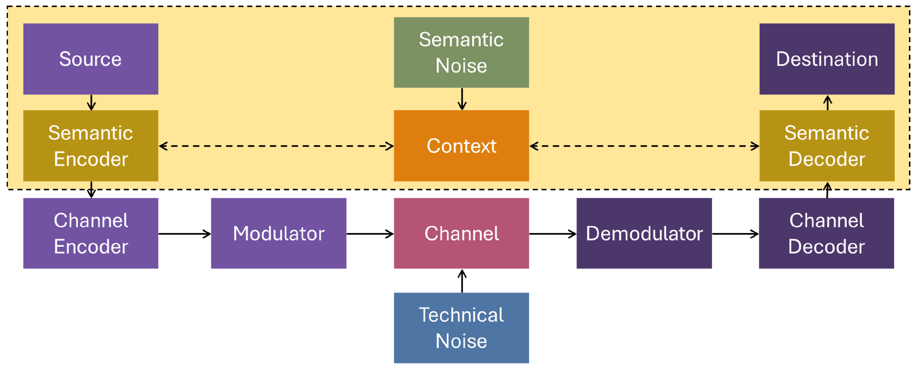
This research aims to develop an autoencoder-based [6] SC system to transmit images over a noisy channel, optimizing bandwidth while maintaining image quality at the receiver for an M2M application. Figure 1 illustrates the SC framework used in this research. A multi-layered autoencoder, which serves as the semantic encoder/decoder pair in this study, generates a latent vector (LV) for a given image. This LV is then channel-encoded before being transmitted over a noisy channel to the decoder. At the decoder, the semantic bitstream is channel-decoded, and the estimated bitstream is used as input to the autoencoder decoder to reconstruct the desired image. Common knowledge, in the form of the dataset on which the autoencoder is trained, is shared between both the encoder and decoder. To reduce the amount of data transmitted, only the LV of a given image is sent through the noisy channel. This approach significantly reduces energy demand and wireless bandwidth usage, contributing to a more sustainable M2M communication network. To protect the LV, we specifically select polar codes as our channel coding scheme, as they demonstrate exceptional performance in achieving channel capacity, offer low-complexity decoding operations, and exhibit resilience against varying channel conditions. The codewords are modulated using the simple yet effective BPSK [7] scheme over a well-studied AWGN channel.

Figure 1. Semantic communication system.

At the receiver end, the noisy LLRs are fed to the decoder, which computes the estimated codewords. We then increase the induced noise in the channel to evaluate the effect of white noise on SC and studied several scenarios. In the first scenario, the autoencoder is trained without any channel noise, and the impact of channel noise on the autoencoder is studied across a range of SNRs. In the second phase, the autoencoder is trained with different levels of channel noise and tested with varying SNRs. In the third scenario, we extend our experiments to include a more complex dataset, where a single decoder is trained under several BERs to observe the impact of operating under different noise levels. In all scenarios, the peak signal-to-noise ratio (PSNR) is calculated for the received images to measure the objective quality of the proposed architecture. Since there are no established semantic quality measurement techniques available, a CNN model is used to identify the semantic meaning of the received images, with its detection accuracy serving as an indicator of the subjective quality. Finally, a comparable JPEG image transmission system (defined in Section 4) is used to benchmark the proposed system. Results indicate that the proposed system outperforms the JPEG-compressed system by up to 17 dB in coding gain.

The main novel contributions of the paper can be summarized as follows:

• A semantically trained autoencoder-based system is proposed for image transmission over resource-constrained, error-prone channels.
• The effect of physical channel noise on designing autoencoder-based SC systems with existing physical communication channels is investigated, and important insights are derived.
• A semantically enabled autoencoder-based image transmission system for M2M communication is demonstrated. The performance of the proposed architecture is compared to a comparable JPEG image transmission system.
• The decoder of the proposed system is trained with noise-added latent vectors, aiding in learning a robust representation.

In summary, we demonstrate that the proposed autoencoder-based SC model can be used in task-oriented M2M communication to convey the semantics of the image under a limited system of resources.

The rest of the paper is organized as follows: Section 2 provides a brief review of the relevant academic literature, covering the theoretical aspects, the use of ML techniques in SC, and the application of autoencoders in image-processing tasks, as well as existing SC-based architectures and their limitations. Section 3 introduces our proposed autoencoder-based SC system, followed by an analysis of the results in Section 4. Finally, conclusions and future work are discussed in Section 5.

2. Related Work

In the development of 6G networks, it is anticipated that SC will become a prominent approach for designing E2E communication systems [8,9,10,11]. SC involves integrating the meaning of the data into various tasks related to processing and transmitting data, which is a significant departure from the traditional Shannon paradigm [5]. Although SC is expected to provide significant advances to emerging modern applications like VIoT, 360° video, AR/VR/MR applications, M2M, and M2H communications, many challenges still exist that must be addressed to make it feasible for real-life applications. These challenges can be divided into the following categories:

• How multimedia data can be effectively compressed to suit SC applications.
• How this source encoding can be better integrated with optimized channel coding for SC applications.
• How these source and channel coding techniques behave under channel noise.
• How SC can be applied in M2M and M2H communications.

The following texts summarize the related work reported on the above challenges and their limitations.

As a starting point, Yang et al. [2] examined the objectives and the strong rationales for implementing SC in 6G networks and presented a summary of the key concepts and crucial technologies that serve as the foundation of SC in 6G networks. Meanwhile, in the field of NLP, deep learning-powered systems have achieved remarkable results in analyzing and comprehending a wide range of linguistic documents. A SC system (DeepSC) introduced in [3] aims for text transmission. Unlike conventional systems that deal with bit or symbol errors, DeepSC aims to recover the meaning of phrases to enhance the system’s capacity and reduce semantic errors. Transfer learning is used to accelerate joint transceiver training and improve the model’s performance in various communication settings. DeepSC-S [4] employs an attention mechanism in the encoder/decoder structure to learn and extract relevant information. The attention mechanism is used to minimize the distortion of the received signal. Results show that DeepSC-S is more robust to channel noise, especially in the low SNR levels. While the above SC systems explore the text data domain, the importance of exploring SC in the multimedia domain has shown great potential.

The authors of [12] consider image corruption during semantic transmission as a form of data augmentation in CL and leverage CL to reduce the semantic distance between the original and the corrupted reconstruction while maintaining the semantic distance among irrelevant images for better discrimination in downstream tasks. The study in [13] proposes a SC system for image transmission that can distinguish between ROI and RONI based on semantic segmentation. The drawback of this method is that it only divides the image into two segments based on bandwidth requirements, not according to the semantic information present. WITT [14] utilizes Swin Transformers as a backbone to extract long-range information specifically optimized for image transmission in wireless channels. WITT introduces a spatial modulation module that scales the latent representations based on channel state information. The above systems propose efficient SC systems to transmit images over noisy channels but have not deeply studied the effect of channel noise on the transmitted semantic data.

Recent advancements in E2E communication systems, which leverage deep learning capabilities, have led to the optimization of transceivers jointly [15,16,17]. These systems integrate all physical layer components, enabling the development of DeepJSCC for image transmission [18]. Unlike conventional systems, this approach does not rely on separate source and channel coding. Instead, the CNN directly maps image bits into channel input symbols. The CNN encoder and decoder are trained jointly, while the communication channel is an untrainable AWGN channel. The autoencoder architecture is used in Deep-JSCC [18] to map the source image directly to channel inputs, and the decoder is trained to reconstruct the image from the input. The proposed method [19] for dimension reduction and image reconstruction involves an architecture that is different from other deep networks that use iterative learning. Instead, the hidden layers of this method are obtained through four distinct steps. This approach results in higher learning efficiency compared to deep networks.

The work in [20] addresses the task of real-time dynamic medical image reconstruction from limited samples, employing an autoencoder to ‘learn’ the reconstruction process from a training set. This approach is based on the ability of neural networks to approximate universal functions. In a similar vein, the article [21] proposes a solution to the image reconstruction problem in ECT using a supervised autoencoder neural network. The proposed network consists of an encoder and a decoder. The authors utilize a simulation-based dataset comprising 40,000 pairs of instances, each containing a capacitance vector and a corresponding permittivity distribution vector, for training and evaluating the autoencoder’s performance. The training and testing are conducted using 10-fold cross-validation on this dataset. While autoencoder-based deep learning techniques have been extensively employed in previous research on image compression, none of these studies have explored autoencoders for source coding under varying levels of physical channel noise.

The work presented in [22] introduces AESC, a SC scheme for wireless relay channels. AESC employs an autoencoder module to encode and decode sentences at the semantic level, ensuring robustness against system noise. Moreover, a semantic forward mode is introduced to enable the relay node to transmit semantic information directly. In the study described in [23], a goal-oriented SC framework is proposed for VANETs. This framework utilizes a DAE to capture semantic information from traffic signs, which is then transmitted to connected autonomous vehicles. In [24], the causes of semantic noise are analyzed, and an adversarial training approach is proposed to incorporate samples with semantic noise into the training dataset. A masked autoencoder is designed as the architecture of a robust SC system, where a portion of the input is masked to mitigate the effect of semantic noise. In [25], a zero-shot learning model based on an SAE is introduced. The SAE model employs a simple and computationally efficient linear projection function and incorporates an additional reconstruction objective to learn a more generalizable projection function. The techniques proposed in [26] focus on transmitting audio semantic information, capturing the contextual features of audio signals. They introduce a wave-to-vector (wav2vec) architecture-based autoencoder, utilizing CNNs to extract semantic information from audio signals. In [27], a CSAEC is presented. CSAEC aims to map data from different modalities to a shared low-dimensional space while preserving semantic information. To achieve this, an autoencoder is employed to establish the association between feature projections and semantic code vectors, considering the similarities across modalities. This approach facilitates the retention of semantic information while aligning representations across different modalities. Notably, none of the mentioned works have explored semantically enabled image transmission over noisy channels.

Therefore, in summary, the existing literature suggests that autoencoders are not typically used for image transmission or SC over a noisy channel, which highlights the main novelty of this paper. On the other hand, in this paper, we address the major issues with our previous work on semantically enabled GAN-based image transmission systems as explained above. A summary of relevant work in SC is provided in Table 1.

Table 1. Summary of relevant work in semantic communication.

Reference	Data Type	Model	Features of the System	Pros	Cons
DeepSC [3]	Text	Autoencoder	Recovers the meaning of phrases to reduce semantic errors	Enhances system capacity, reduces semantic errors	Limited to text transmission
DeepSC-S [4]	Text	Autoencoder	Uses the attention mechanism to minimize signal distortion	Robust to channel noise, especially in low SNR regimes	Focused on text data only
Luo et al. [22]	Text	Autoencoder	AESC for wireless relay channels, robust against noise	Introduces the semantic forward mode	Focused on text, not multimedia
Tang et al. [12]	Image	Autoencoder	Leverages CL to minimize semantic distance	Improves discrimination in downstream tasks	Limited exploration of channel noise effects
Bourtsoulatze et al. [18]	Image	Autoencoder	Joint source-channel coding without separate coding	Efficient image transmission	Does not study varying physical channel noise
DeepJSCC [18]	Image	Autoencoder	Maps images to channel inputs, reconstructs from noisy channel output, joint source-channel coding	Robust image reconstruction	Limited exploration under different noise conditions
Mehta et al. [20]	Image	Autoencoder	Real-time dynamic medical image reconstruction	High learning efficiency	Does not consider channel noise in source coding
Zheng et al. [21]	Image	Autoencoder	Image reconstruction in ECT using supervised learning	High accuracy in specific domain	Limited to ECT, no channel noise exploration
Rahagoal [23]	Image	Autoencoder	Goal-oriented SC for VANETs using DAE	Captures semantic info from traffic signs	Limited to traffic sign data, not generalizable
Hu et al. [24]	Image	Autoencoder	Robust SC with adversarial training against semantic noise	Incorporates semantic noise in training	Focused on robustness, not general image transmission
Kodirov et al. [25]	Image	Autoencoder	Zero-shot learning with semantic autoencoder (SAE)	Efficient, generalizable projection function	Not focused on image transmission over noisy channels
Wu et al. [13]	Image	CNN	Semantic segmentation to distinguish ROI and RONI	Efficient bandwidth usage	Limited by segmentation based on bandwidth, not semantics
WITT [14]	Image	Transformer	Uses Swin Transformers, spatial modulation based on channel state	Extracts long-range information, optimized for wireless channels	Channel noise effects on semantic data not deeply explored
GAN-based SC [28]	Image	GAN	GAN generates images based on semantic map	Can generate images similar to style images	High sensitivity to channel errors, unsuitable for task-oriented M2M
semantIC [29]	Text	Neural Network-based Semantic Interference Cancellation	Utilizes Wyner-Ziv theorem and side information to reduce interference in 6G wireless communication	Improves decoding accuracy, robust against interference	Complex implementation, high computational cost
Autoencoder-based relay [22]	Text	Autoencoder with Relay Channels	Introduces relay channels for better transmission in semantic communication systems	Improves transmission reliability over long distances, reduces semantic errors	Increased complexity due to relay channel coordination
Joint coding- modulation [30]	Digital Symbols	Variational Autoencoder	Jointly optimize coding and modulation using variational inference to maximize mutual information	Robust against channel noise, improves semantic and data recovery accuracy	Computationally intensive, requires complex decoder design

The proposed system reconstructs the image using its latent representation, which can lead to significantly higher compression gains compared to traditional image compression systems while maintaining the expected quality. It transmits images across a noisy channel and receives them at the receiver with reduced semantic noise. The proposed system considers an M2M application to demonstrate the impact of these technologies. The proposed architecture is highly robust against channel noise and performs significantly better in terms of objective and subjective quality compared to a comparable JPEG-based image transmission system (defined in Section 4). The next section presents the proposed framework in detail.

3. Proposed Autoencoder-Based Image Transmission System

The mathematical model for the proposed architecture is presented in the section below:

$$\mathbf{h}=f({\mathbf{W}}_{\mathrm{enc}}·\mathbf{x}+{\mathbf{b}}_{\mathrm{enc}}).$$

(1)

Equation (1) represents the encoder function, where $\mathbf{x}\in {\mathbb{R}}^{mn\times c}$ is the input data. Here, m and n denote the height and width of the input image, respectively, and c denotes the number of color channels. ${\mathbf{W}}_{\mathrm{enc}}\in {\mathbb{R}}^{p\times mn\times c}$ is the encoder weight matrix, ${\mathbf{b}}_{\mathrm{enc}}\in {\mathbb{R}}^{p\times 1}$ is the encoder bias vector, $\mathbf{h}\in {\mathbb{R}}^{p\times 1}$ represents the latent vector where p is much smaller than $mn\times c$, and $f(.)$ denotes the activation function.

$$\widehat{\mathbf{x}}=f({\mathbf{W}}_{\mathrm{dec}}·\mathbf{h}+{\mathbf{b}}_{\mathrm{dec}}).$$

(2)

Equation (2) represents the decoder function, where $\widehat{\mathbf{x}}\in {\mathbb{R}}^{mn\times c}$ is the reconstructed output, $\mathbf{h}\in {\mathbb{R}}^{p\times 1}$ is the latent vector, ${\mathbf{W}}_{\mathrm{dec}}\in {\mathbb{R}}^{mn\times c\times p}$ is the decoder weight matrix, ${\mathbf{b}}_{\mathrm{dec}}\in {\mathbb{R}}^{mn\times c}$ is the decoder bias vector, and $f(.)$ denotes the activation function.

$$\mathcal{L}(x,\widehat{x})=-\left(xlog\left(\widehat{x}\right)+(1-x)log(1-\widehat{x})\right).$$

(3)

In Equation (3), $\mathcal{L}(.)$ denotes the binary cross-entropy loss, which represents the true binary label (0 or 1), and $\widehat{\mathbf{x}}\in {\mathbb{R}}^{mn\times c}$ indicates the predicted probability of the positive class (between 0 and 1).

$$\widehat{\mathbf{y}}=f({\mathbf{W}}_{\mathrm{dec}}·\widehat{\mathbf{h}}+{\mathbf{b}}_{\mathrm{dec}}).$$

(4)

The equation to train the decoder with a noisy latent vector is defined in (4), where $\widehat{\mathbf{y}}\in {\mathbb{R}}^{mn\times c}$ represents the reconstructed output, ${\mathbf{W}}_{\mathrm{dec}}\in {\mathbb{R}}^{mn\times c\times p}$ is the weight matrix of the decoder, ${\mathbf{b}}_{\mathrm{dec}}\in {\mathbb{R}}^{mn\times c}$ is the bias vector of the decoder, and $\widehat{\mathbf{h}}\in {\mathbb{R}}^{p\times 1}$ is the noise added latent vector. The noise is typically applied to the latent vector before passing it to the decoder, aiding in learning a robust representation.

$$\widehat{\mathbf{h}}=\mathbf{h}+\mathcal{N}(0,{\sigma }^2).$$

(5)

Equation (5) illustrates how $\mathbf{h}\in {\mathbb{R}}^{p\times 1}$ and $\widehat{\mathbf{h}}\in {\mathbb{R}}^{p\times 1}$ are related through the AWGN distribution with 0 mean and ${\sigma }^2$ variance.

The following subsections illustrate the main features of the proposed autoencoder-based image transmission system.

3.1. Semantic Encoder Architecture

Figure 2 presents the proposed encoder used in the autoencoder. As shown in the figure, the first layer of the encoder is a convolution layer with 32 filters (kernels), having dimensions of $3\times 3$ with one channel. The combination and nature of convolutional layers, max pooling layers, activation functions, dense layers, and vector spaces are optimized for the application under consideration to minimize system resource usage. Padding is added to the input volume as the “same” value, and the stride of the convolution operation is set to 1 such that the output volume has the same spatial dimensions as the input volume. Max pooling is used next with a pool size of $2\times 2$. It decreases feature maps by a factor of two in both height and width dimensions. This is considered the first convolutional layer up to this point. During the second convolutional layer, 64 filters that have the dimensions of $3\times 3$ with 32 channels are employed. The use of 64 filters in the second convolutional layer will improve the ability to extract high-level features from the input data. As the network grows, the number of functions learned at each layer becomes more abstract and advanced. More filters in the second convolutional layer allow the network to capture more complex and detailed features in the input data. Similar to the first convolutional layer, max pooling is performed on the second convolutional layer, and the feature maps are downsampled to a size of $7\times 7$ with 64 channels. The flatten function is used to convert the output of the second convolutional layer into a one-dimensional array with the shape of 3136 by 1, which can then be fed into the fully connected layers. Finally, another dense layer is created as the bottleneck (latent vector) of the autoencoder with the ReLU activation function, which produces the final encoded representation with a shape of $32\times 1$. Though several images are analyzed, within the presentation of this paper, only $28\times 28$ images from the MISNT [31] dataset are considered. The keras [32] library is used to implement the autoencoder in Python.

Figure 2. Proposed encoder in the autoencoder.

3.2. Semantic Decoder Architecture

To develop a comprehensive autoencoder model, the accompanying decoder layers must also be defined in line with the encoder model described in the previous section. Figure 3 illustrates the proposed decoder architecture to use in the autoencoder. As shown in Figure 3, with the $32\times 1$ latent vector, a dense layer in the shape of $3136\times 1$ is defined with the ReLU activation function. The dense representation is then reshaped into a 3D tensor with a shape of $7\times 7$ with 64 channels, which is then fed into two deconvolutional layers with two up-sampling layers to reconstruct the original input image with one channel. The final layer of the decoder uses the sigmoid activation function. Finally, the autoencoder model is then defined as a sequential model by combining the encoder and decoder layers. It is then compiled with the Adam optimizer with a learning rate of $0.001$ and a binary cross-entropy loss function before training the model. The training data are used for both the input and the output.

Figure 3. The proposed Decoder in the Autoencoder.

The hyperparameters chosen for the autoencoder model—such as the number of filters, kernel size, activation functions, learning rate, and loss function—are determined based on extensive experimental testing and optimization. These experiments are conducted to ensure that the model achieves the best possible performance while remaining computationally efficient.

3.3. Dataset Description and Data Preprocessing

Within this research, we use two different datasets to evaluate the effectiveness of the proposed framework.

The MNIST dataset consists of a training set of 20,000 images and a testing set of 10,000 images, each of which is 28 × 28 pixels in size, totaling 784 pixels per image. Each pixel has a value ranging from 0 to 255. By dividing each pixel value by the maximum value (255), the pixel values in each image are normalized to a range of 0 to 1. This normalization helps ensure that the data are on the same scale, which can improve the model’s performance. The dataset is reshaped into a three-dimensional array with dimensions 28 × 28 × 1. Since the images are grayscale, the 1 at the end indicates the number of color channels. To augment the dataset, random noise is added to the 20,000 training images to create a new set of 80,000 training images.

The CIFAR-10 [33] dataset consists of 60,000 color images across 10 classes. Each CIFAR-10 image is 32 × 32 pixels in size. Similar to the MNIST dataset, CIFAR-10 pixel values range from 0 to 255 and are typically normalized to a range of 0 to 1 by dividing by 255. CIFAR-10 images are in RGB format, resulting in data dimensions of 32 × 32 × 3. The CIFAR-10 dataset contains 50,000 training images and 10,000 testing images.

3.4. Training Process

Initially, the model is trained with no noise. The defined autoencoder model is compiled with an optimizer and loss function and trained on the data for 15 epochs with a batch size of 50. The Adam optimizer is used with a learning rate of $0.001$. Since the last deconvolutional layer of the decoder has a sigmoid activation function, the output of the final layer is a number between 0 and 1 for each node, which is why binary cross-entropy is chosen as the loss function. To train only the decoder, the encoder’s predicted data must be used as the decoder’s input data. Since the encoder and decoder layers are defined independently in the autoencoder model, a new model can be created that only contains the encoder layers. Then, the encoder model can predict the data for the training dataset. After obtaining the encoder output data for the training dataset, the data are modified thereafter by the addition of different noises. In the proposed system, 80,000 training latent vector sets are created for each BER considered. Listed below are the different BERs for which the latent vectors are created. Based on the hyperparameter selected, BERs of $0.0\%$, $0.625\%$, $1.25\%$, $1.875\%$, $2.5\%$, $3.125\%$, $3.75\%$, and $4.375\%$ are considered in the rest of the paper. However, it should be noted that any other BERs can be selected for training the AE based on external parameters. After obtaining those eight datasets, each containing 80,000 latent vectors, eight different decoders are individually trained.

3.5. Proposed End-to-End M2M Communication System

Figure 4 illustrates the proposed E2E M2M communication system. As explained earlier, the semantic encoder and the semantic decoder of the proposed autoencoder are placed at the transmitter and the receiver, respectively. The transmitter consists of an encoder followed by a polar channel encoder and a BPSK modulator. The modulated signal is transmitted over an AWGN channel and demodulated by a BPSK demodulator and a polar channel decoder followed by the decoder. The selection of the channel coding and modulation scheme is independent of the proposed autoencoder design and its E2E performance analysis since the objective of this paper is to consider the E2E autoencoder-based semantic image transmission system for M2M applications. Finally, the transmitted image and the received images are compared with an image objective quality metric (PSNR). The following subsections explain the other main details which are relevant to the proposed design.

Figure 4. Proposed end-to-end M2M communication system.

3.6. Machine Perception of Images

Since there is no widely recognized image quality metric specifically designed for machines and SCs, another CNN model is trained to evaluate the received images based on their classification accuracy. Classification accuracy is a critical metric, as it directly reflects the machine’s ability to interpret and act on the transmitted information. This approach ensures that the system’s performance is measured not just by traditional image quality metrics but by how effectively it enables machines to extract and utilize the intended semantic content from the images. Figure 5 demonstrates the proposed CNN image classification model to perceive the images. As shown in Figure 5, the input shape of $(28,28,1)$, two convolutional layers (kernel size = $(3,3)$) with a ReLU activation function, two max pooling layers (pool size = $(2,2)$), and three dense layers with a ReLU activation function, followed by a final dense layer with a sigmoid activation function, are used for the CNN classification test setup.

Figure 5. Proposed CNN model for image classification.

The main idea is to transfer the latent vector through a channel and determine what it implies from the M2M perspective after reconstructing it from the transmission. Since the idea of the SC is to increase the actual information content at a lower data rate, the autoencoder can be used to transmit the minimum number of bits while preserving the original quality of the data. The encoder takes the input data and compresses them into a lower-dimensional representation. The latent vector is then transferred through a channel. On the receiver side, the decoder takes the compressed representation and reconstructs the original data. The reconstructed data are used for image recognition via CNN as shown in Figure 5.

3.7. Communication Framework

Polar codes, a significant development in coding theory, are denoted by the notation $\mathcal{PC}(N,K)$, where N and K respectively represent the block length and the number of message bits. The concept of channel polarization, introduced by Arikan [34], involves the transformation of a physical channel into highly reliable and highly unreliable virtual channels as the code length grows toward infinity. This technique has been proposed as an effective method to improve the reliability and efficiency of communication systems. Several studies, such as [35,36,37], have demonstrated the efficacy of polar codes in achieving high throughput or low latency, making them a promising solution for various communication applications. Polar codes can leverage the identification of the most reliable channels by using Bhattacharya parameters [34] or Gaussian approximation [38]. Subsequently, these favorable positions can be utilized for embedding the information bits.

The specification of the channel coding scheme used in this paper is elaborated in Table 2, outlining the intricate details of the selected scheme. Polar codes under successive cancellation algorithms are selected as our preferred channel coding scheme. A polar code of size $N=2048$ with rate $R=0.78$ is chosen to validate the proposed SC system. Like the methodology employed in [28], the selected polar code is optimized for an SNR of $2.5$ dB, where the codewords are modulated utilizing BPSK across an AWGN channel. Finally, a quantization scheme involving 5 bits is employed to encode the pixel values, allowing the output image layer to be transmitted in a single packet. At the receiver end, the noisy LLRs are processed by the polar decoder, which computes the estimated codewords. The BER and FER of the selected polar code are depicted in Figure 6. Obviously, as the SNR grows, the error rate decreases. Based on this observation, it can be inferred that the BER becomes practically negligible in our specific application at an SNR of 4 dB or higher since the robustness of the latent vector can tolerate the BER values of more than 10⁻³. This can be further explained in Figure 7 where PSNR achieves its maximum value above 4 dB.

Table 2. Channel encoding/decoding setup.

Parameter	Value
Channel en/decoder	Polar Code
Decoding algorithm	Successive-Cancellation
Number of information bits (N)	1600
Number of codeword bits (K)	2048
Code Rate (R)	$0.78$
Image resolution	$10\times 32$
Number of bits used for quantization (Q)	5
Modulation scheme	BPSK
Number of bits per symbol	2
Demapping method	LLRs
Channel Type	AWGN

Figure 6. The error correction performance of $\mathcal{PC}(2048,1600)$.

Figure 7. SNR against PSNR.

4. Results

This section discusses the simulation results of the proposed autoencoder-based image communication system presented in Section 3. PSNR and classification accuracy are considered under different channel SNR conditions over a range of different images to measure the efficacy of the proposed architecture. Finally, the performance is compared against an equivalent JPEG-based image communication system to complete the study. The equivalent JPEG system is defined such that the bitrate of both systems is approximately maintained at the same level.

4.1. Analyzing the Image Quality of the Proposed System Under Different Channel SNRs

PSNR between the received and transmitted images is used as an objective metric to evaluate the performance of decoders in the proposed autoencoder-based M2M communication system. Figure 7 illustrates how PSNR varies across different channel SNR levels under various trained decoders. The simulation considered SNR levels of 2.5, 3.0, 3.5, 4.0, and 4.5 dB, representing different qualities of the transmitted signal. At an SNR of 2.5 dB, the simulation recorded a very high BER. As the SNR increases to 3.0 dB and 3.5 dB, the BER reduces, indicating more reliable transmission. At an SNR of 4 dB or higher, the BER becomes negligible, indicating error-free transmission.

The results show that each decoder reaches its saturation point at high SNRs. When the SNR is low, each decoder shows low PSNR levels, indicating that the reconstructed signal differs significantly from the original signal. This is expected because a low SNR implies a high noise level, making it difficult for the decoder to accurately reconstruct the original signal. When the SNR is moderate, the decoder trained with zero BER has a lower PSNR level compared to other decoders. This shows that, despite performing well at high SNR values, the decoder trained with zero BER may not operate well in a low noise-level channel.

Figure 7 also shows that the channel decoder successfully recovers nearly all the bits transmitted through the channel at an SNR of 4 dB or above. However, the receiver PSNR saturates at 22 dB at high SNRs because the AE cannot be trained to predict the exact image, resulting in a residual error. This residual error is the semantic noise carried forward at the receiver. Therefore, the maximum achievable quality is 22 dB PSNR. While 22 dB PSNR might seem low for human perception, it is sufficient for machine perception. As demonstrated later, the image classification model can still accurately identify the intended meaning of the message, indicating that this level of quality is adequate for machine vision applications.

4.2. Analyzing the Classification Accuracy of the Proposed System Under Different Channel SNRs

As explained in Section 3 under the methodology, since no image quality metrics are available for machine perception of a semantically transmitted image, a CNN model is used for image classification to emulate machine perception. Figure 3 shows how the CNN classification accuracy varies under different channel SNRs with various trained decoders. The simulation is conducted at the same SNR levels as those shown in Figure 8. At low SNRs (less than 2.5 dB), all trained decoders exhibit very low classification accuracy. At medium channel SNRs (3 dB to 3.5 dB), decoders trained with different channel errors achieve the best classification accuracy, while the decoder trained with zero error fails to perform effectively. At high SNRs (greater than 3.5 dB), all trained decoders achieve very high classification accuracy. Moreover, at high channel SNRs, all decoders perform similarly, regardless of their training conditions.

Figure 8. SNR against accuracy (CNN for digit classification).

4.3. Analyzing the Image Quality of the Proposed System Under Different BERs

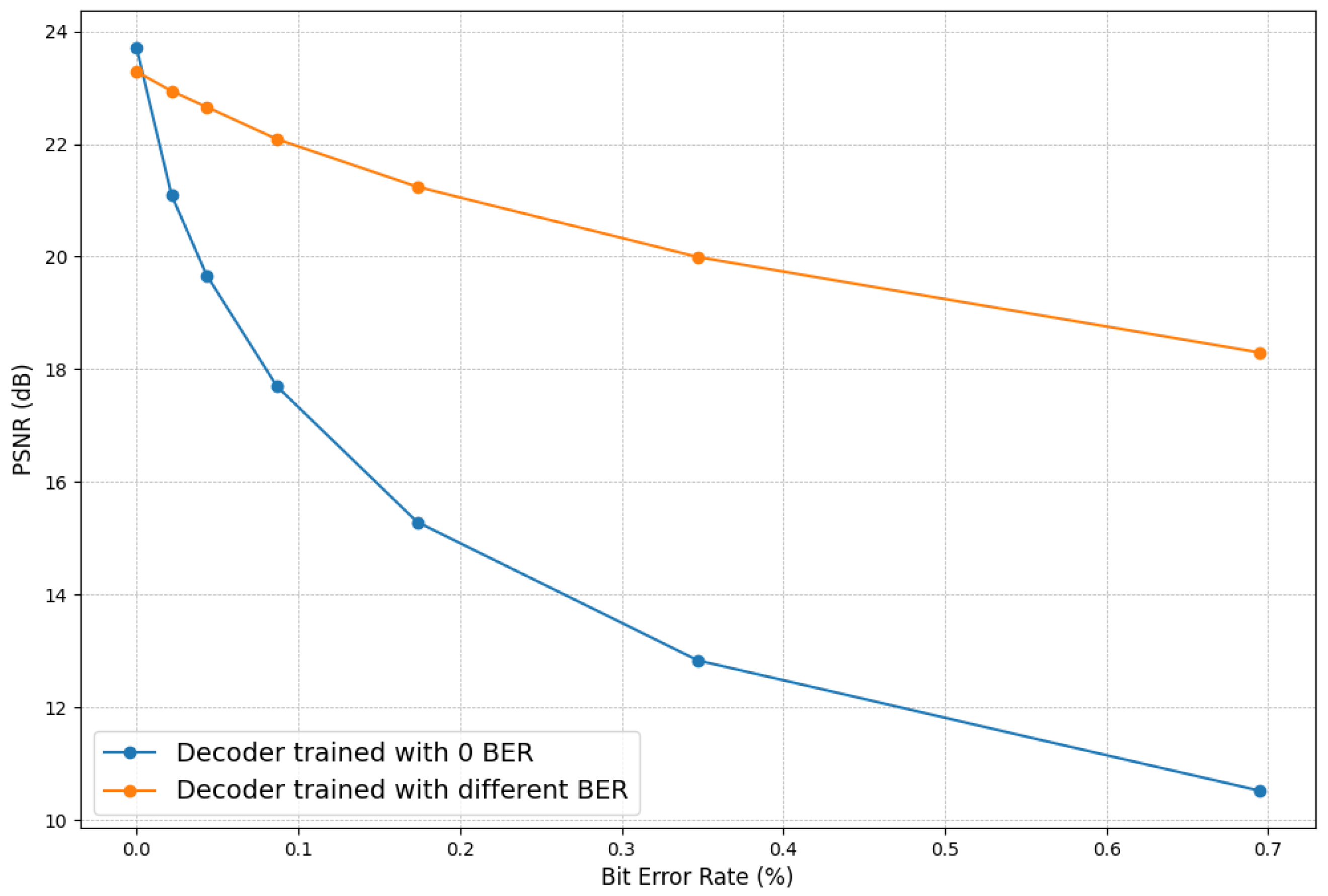
Figure 9 illustrates the quality of received images for a range of BERs (0 to $37.3\%$) under different trained decoders. The observation shows that each decoder has high PSNR levels at zero BER, but the decoders trained with different noise levels have lower PSNR levels compared to the decoder trained with no noise. As the BER increases, the PSNR of the decoder trained with no noise decreases significantly compared to the other decoders. All other decoders have more or less similar performance, indicating that their behavior is mostly independent of the noise levels they were trained with.

Figure 9. BER against PSNR.

4.4. Analyzing the Image Classification Accuracy of the Proposed System Under Different BERs

Figure 10 presents CNN image classification accuracy for different BER levels (from 0 to $4.375\%$ BER) under different trained autoencoders. The observation shows that each decoder has high accuracy levels at zero BER. At high BERs, the decoder trained with no noise performs worse compared to the other decoders, whereas all other decoder types demonstrate similar performances. This observation suggests that decoders trained with different noise levels have marginal improvements in classification accuracy under varying channel BERs.

Figure 10. BER against accuracy (CNN digit classification).

4.5. Analyzing the Image Quality and Image Classification Accuracy of the Proposed System Under Different BERs with the CIFAR-10 Dataset

In this experiment, we analyzed the impact of a complex dataset by training a single decoder under several BERs to observe the effects of different noise levels. Figure 11 and Figure 12 present the PSNR and CNN image classification accuracy for different BER levels (ranging from $0\%$ to $0.7\%$ BER) using the CIFAR-10 dataset, with the decoder trained at various BERs. Similar to Figure 9 and Figure 10, the results show that each decoder achieves high accuracy and PSNR at zero BER. However, at high BERs, the decoder trained without noise performs worse compared to the proposed decoder. This suggests that decoders trained with different noise levels exhibit improvements in both classification accuracy and PSNR under varying channel BERs.

Figure 11. BER against PSNR (CIFAR-10 dataset).

Figure 12. BER against accuracy (CNN classes classification—CIFAR-10 dataset).

This approach demonstrates the decoder’s ability to handle varying BERs with a similarly trained model. The results indicate the robustness of a single decoder model across a range of noise levels and its capability to adapt to different BERs when processing semantically communicated information.

4.6. Performance Comparison Against JPEG Image Transmission

The performance of the proposed communication system is compared against a JPEG-based communication system under similar constraints. With the proposed autoencoder, the images are compressed by a factor of approximately 40 (0.2 bits per pixel), whereas JPEG manages to compress the images by only a factor of 20 (0.4 bits per pixel) while maintaining reasonable image quality. The JPEG encoder generates the JPEG-compressed bit stream, which is then transmitted over the same AWGN channels under the same channel and modulation types used with the proposed E2E system. Figure 13 and Figure 14 present the performance comparison between the proposed and JPEG systems. A compression factor of 20 is the lowest achievable with the JPEG encoder. Below 4.0 dB, the JPEG system fails to maintain any image quality, while the proposed autoencoder-based system continues to perform well. Even at high SNRs (above 3.5 dB), JPEG produces poor image quality compared to the proposed autoencoder-based system due to the excessive quantization noise. As in conventional communication systems, the performance of our system declines under low SNR conditions due to the combined effects of technical noise and semantic noise. However, it is important to emphasize that the impact of technical noise in our system is considerably lower compared to conventional systems like JPEG. Despite the degradation at low SNRs, our approach remains more resilient. In Section 4, we demonstrate that the proposed approach achieves up to 17 dB coding gain at mid SNRs (3 dB) compared to the JPEG system. Finally, it should be noted that this is achieved at a lower compression ratio, meaning JPEG consumes much higher bandwidth yet results in inferior image quality at the receiver.

Figure 13. Performance comparison of the proposed system versus JPEG (SNR vs. PSNR).

Figure 14. Performance comparison of the proposed system versus JPEG (BER vs. PSNR).

4.7. The Performance as a Function of the Compression Ratio, Specifically Varying the Dimension of the Latent Vector

The diagram in Figure 15 shows the performance of an image transmission system as a function of the compression ratio, specifically varying the dimension of the latent vector (LV size). Diagram (a) illustrates how the PSNR changes with varying LV sizes. As the LV size increases, the PSNR also increases, indicating higher image quality but plateaus around LV size 30–50, showing diminishing returns. Diagram (b) shows how the accuracy of a CNN image classification model varies with LV size. Classification accuracy rises sharply with an increase in LV size up to about 30, beyond which gains are marginal. This suggests that a latent vector size of around 30–40 is sufficient for achieving near-optimal classification accuracy.

Figure 15. Effect of the LV size on (a) PSNR and (b) accuracy of prediction.

Extensive experiments determined the optimal LV size to minimize the bitrate while maintaining image quality. An LV size of around 30–40 provides a good trade-off between compression and quality (both in terms of PSNR and classification accuracy). This enables efficient image transmission in resource-constrained environments, ensuring image reconstruction and accurate image classification with minimal data rates.

4.8. Computational Complexity

While the proposed autoencoder-based system is computationally expensive compared to the JPEG system during the initial phase, this is due to the extensive training required at the beginning. However, it is important to note that the model is trained only once during the development phase. After this one-time training, the model is deployed and used for inference, which is significantly less computationally demanding. The computational intensity is primarily confined to the training stage, which can be performed using high-performance computing resources. Once deployed, the system only requires forward passes through the trained model for encoding and decoding. This makes it highly feasible for use in resource-constrained environments during the deployment phase.

5. Conclusions and Future Work

This paper proposes an autoencoder-based semantic image communication system that compresses and transmits images over an error-prone channel, with the goal of decoding and reconstructing the original data at the receiver under varying channel noise levels. To exploit the semantics of the information, joint training of the encoder and decoder in the autoencoder is performed, generating a highly reduced dimensional vector called the latent vector. Once trained, the encoder and decoder are placed at the transmitter and receiver, respectively. The transceivers are connected through an error-prone channel, and the latent vector is transmitted over this channel under different SNRs. A polar channel encoder and a BPSK modulator are used on the transmitter side, with corresponding decoders/demodulators at the receiver. The proposed autoencoder is trained under different channel noise levels to minimize reconstruction error at the decoder, enabling it to better reconstruct the original data from noisy inputs. This approach ultimately improves the system’s performance in noisy channels.

The simulation results illustrate that the proposed system maintains excellent image quality and very high classification accuracy above 3.5 dB channel SNR. Below 3.5 dB, the autoencoder trained with different noise levels performs much better than the autoencoder trained with zero errors. The reason for this behavior is that channel errors introduced during training helped the model mitigate the impact of channel noise at lower SNRs. All autoencoders fail to produce good image quality at very low channel SNRs. This is expected, as in any communication system, where decoders struggle to reconstruct images at low SNRs. The results are compared against an equivalent JPEG transmission system, showing that the proposed system’s performance is far superior to the JPEG system across all channel SNRs under similar constraints. Both image quality and compression performance are significantly better in the proposed system than in the JPEG system. We also tested the proposed framework on a complex dataset, as explained in Section 2, and observed similar performance enhancements. Therefore, we can conclude that the proposed SC system is independent of specific datasets and performs equally well under various conditions.

Future work will aim to more comprehensively represent the complexities of real-world images, better reflecting the diversity and challenges encountered in practical applications. The concept and approach presented in this paper are not limited to these datasets. We chose MNIST and CIFAR-10 as representative benchmarks. The experiments conducted on these two datasets serve to validate the methodology, and the same principles can be extended to more complex datasets in future work. Furthermore, we plan to extend this work by implementing a scalable semantic image communication system that can operate efficiently over error-prone channels. Additionally, we aim to develop a similar system for video transmission.