Polynomial Time Algorithm for Shortest Paths in Interval Temporal Graphs ^†

Abstract

We develop a polynomial time algorithm for the single-source all destinations shortest paths problem for interval temporal graphs ($ITG$s). While a polynomial time algorithm for this problem is known for contact sequence temporal graphs ($CSG$s), no such prior algorithm is known for $ITG$s. We benchmark our $ITG$ algorithm against that for $CSG$s using datasets that can be solved using either algorithm. Using synthetic datasets, experimentally, we show that our algorithm for $ITG$s obtains a speedup of up to $32.5$ relative to the state-of-the-art algorithm for $CSG$s.

1. Introduction

Temporal graphs are dynamic graphs that can change over time. Edges and Vertices in a temporal graph may evolve over time and thus have temporal information associated with them. Temporal graphs can be used to model many real-world problems such as modeling the spread of viral diseases, traffic flow in road networks, information flow in social networks and other such problems representing dynamic connectivity [1,2,3,4,5,6,7]. Recently, temporal graphs have been used in machine learning as temporal graph neural networks ($TGN$s) [8].

Different models can be used to represent a temporal graph [3]. One such popular model is a contact sequence temporal graph ($CSG$). Every instance of time when a communication can be initiated from a vertex u to a vertex v is represented by a unique temporal edge $(u,v,t,\lambda )$ in the $CSG$ model. t is the departure time and $\lambda$ is the travel time along this edge, such that the arrival time at v when departing u along this edge would be $t+\lambda$. Figure 1 shows an example of a $CSG$.

Figure 1. Contact sequence temporal graph.

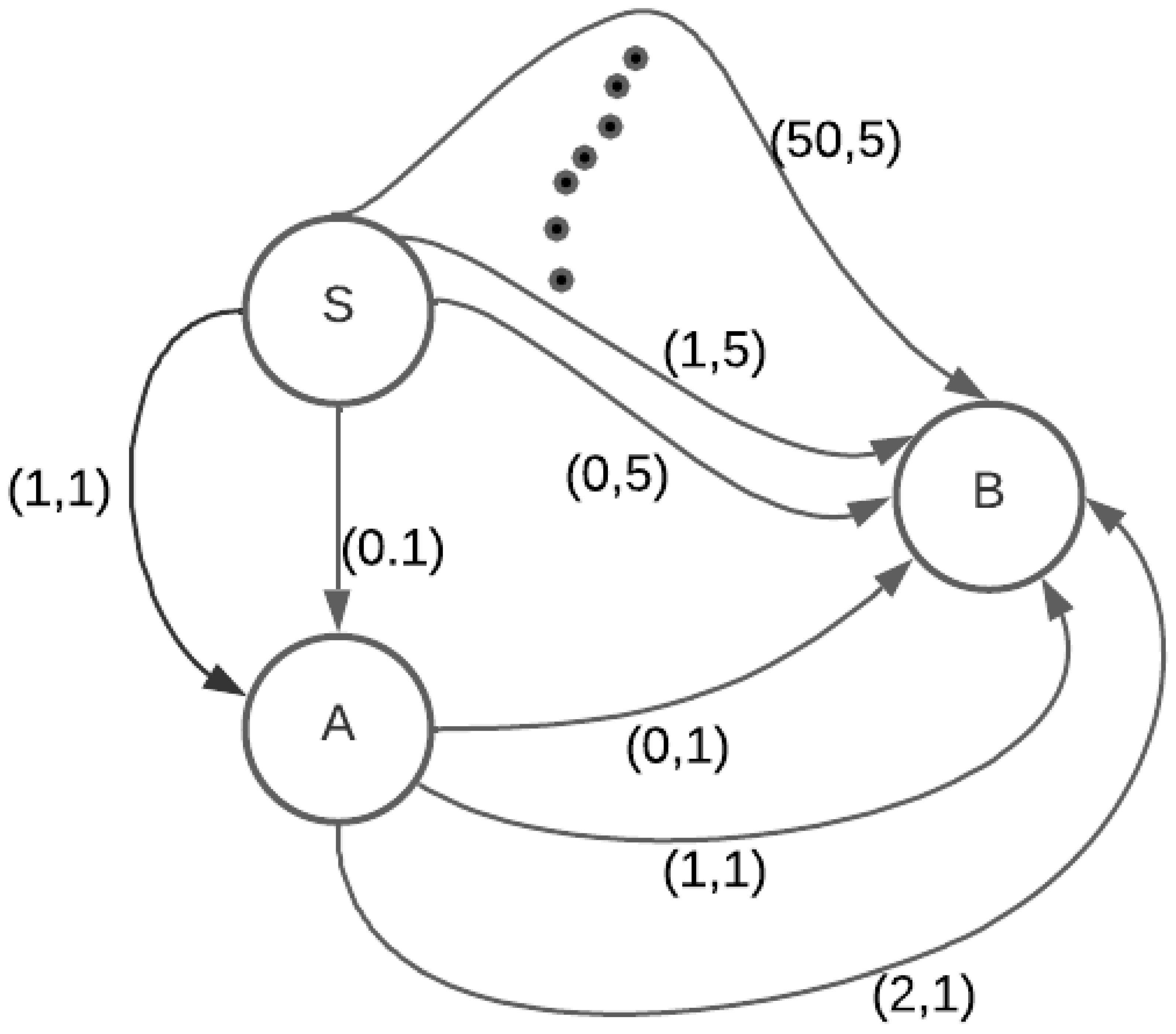
An alternate representation of a temporal graph is an interval temporal graph ($ITG$). Temporal information on an edge connecting two vertices $(u,v)$ in an $ITG$ is modeled as a vector of contiguous time intervals $i=(s_i,c_i)$, with an associated travel time ${\lambda }_i$ for each interval i. Figure 2 illustrates an example of an $ITG$. Communication from u to v may be initiated at any time t such that $s_i\le t\le c_i$ for one of the intervals i along this edge.

Figure 2. Interval temporal graph.

While every CSG has an equivalent ITG, the reverse is true only when time is discrete.

Some applications of temporal graphs are described below:

• Intelligent Transportation Systems—Road networks can be modeled by temporal graphs where vertices represent street intersections [9]. Varying traffic and street conditions are represented as temporal edges. Such temporal graphs enable building intelligence in transportation systems to improve safety, mobility and efficiency.
• E-health and bioinformatics—Temporal graphs can be used to model pandemic spread by building proximity networks [10,11,12]. This kind of modeling can help understand the source of pandemic spread and the best methods to contain the pandemic spread.
• Social Networks—Social networks are usually large dynamic graphs. Refs. [1,13] present a framework for modeling social networks. Santoro et al. [5] propose an approach for studying temporal metrics in social graphs using temporal graphs.
• Artificial Intelligence—Graph Neural Networks (GNNs) have become popular in recent times due to their ability to learn complex systems of relations or interactions. They provide a framework for deep learning models on graphs. Recently, new frameworks have been proposed for deep learning on dynamic or temporal graphs. For example, Rossi et al. [8] propose a framework for deep learning on temporal graphs that they call Temporal Graph Networks (TGNs). Smith et al. [14] propose a novel architecture for online learning with temporal neural networks.

Path and walk problems on temporal graphs are studied, for example, in [9,15,16,17,18,19,20]. While [16,18,19] focus on $ITG$s, Refs. [15,17,20,21] use the $CSG$ model. Wu et al. [15] demonstrate that the studied path problems can be solved faster using the algorithms proposed by them on the $CSG$ representation when compared to the algorithms proposed on the $ITG$ representation by Xuan et al. [16]. However, Jain et al. [18,19] subsequently developed algorithms for $ITG$s that outperform the $CSG$ algorithms of Wu et al. [15] for most of the studied path problems as well as the ITG algorithms of Xuan et al. [16]. Gheibi et al. [20] proposed an alternate TRG data structure for representing $CSG$s that results in faster algorithms than the algorithms of Wu et al. [15] for most of the studied path problems.

Bentert et al. [17] developed a polynomial time algorithm, for $CSG$s, to compute walks that optimize any linear combination of the optimization criteria studied by [15,16,18,20] with min and max waiting time constraints at each vertex. Jain et al. [19] show that a linear combination of multiple criteria can be used to find walks and paths with a secondary optimization criterion for, e.g., min-hop foremost ($mhf$) paths or min-wait foremost ($mwf$) walks.

Jain et al. [19] present algorithms for dual criteria $min-hop-foremost$ ($mhf$) and $min-wait-foremost$ ($mwf$) for $ITG$s. Their ITG algorithms solve the $mhf$ and $mwf$ problems in less time than when the algorithm of Bentert et al. [17] is used on the corresponding CSGs and the coefficients of the linear combination optimization criteria in Bentert et al.’s algorithm are chosen so as to compute $mhf$ and $mwf$ walks. Jain et al. [21] also develop an algorithm to compute walks optimizing any linear combination of the criteria considered by Bentert et al. [17] with waiting time constraints, outperforming the algorithm by Bentert et al. by up to a factor of 77. However, the limitation of the algorithm by Jain et al. is that it only works on $CSG$s with no zero-duration cycle.

In this paper, we develop an algorithm to find the shortest paths in $ITG$s. A shortest path between any two vertices A and B in a temporal graph is a feasible path for which the travel time to reach from A to B is minimum. Xuan et al. [16] propose a polynomial time algorithm to find min-hop paths in $ITG$s. A min-hop path from vertex A to B is a feasible path that travels through the minimum number of edges to reach B. Such a path is also the shortest path from A to B when all edges have the same travel time. However, in general, travel times on the edges of an interval temporal graph may be different. No algorithm has been proposed for finding the shortest paths when the temporal graph is expressed as an $ITG$. Wu et al. [15], Bentert et al. [17], Jain et al. [21] and others proposed algorithms that can be used to find the shortest paths when temporal graphs are expressed as $CSG$s. As noted earlier, $ITG$s cannot be expressed as $CSG$s when time is continuous. Further, even when time is discrete, the size of the $CSG$ corresponding to a given $ITG$ could be quite large (when the time intervals of edges are large). This paper fills this gap by providing a polynomial time shortest path algorithm for $ITG$s.

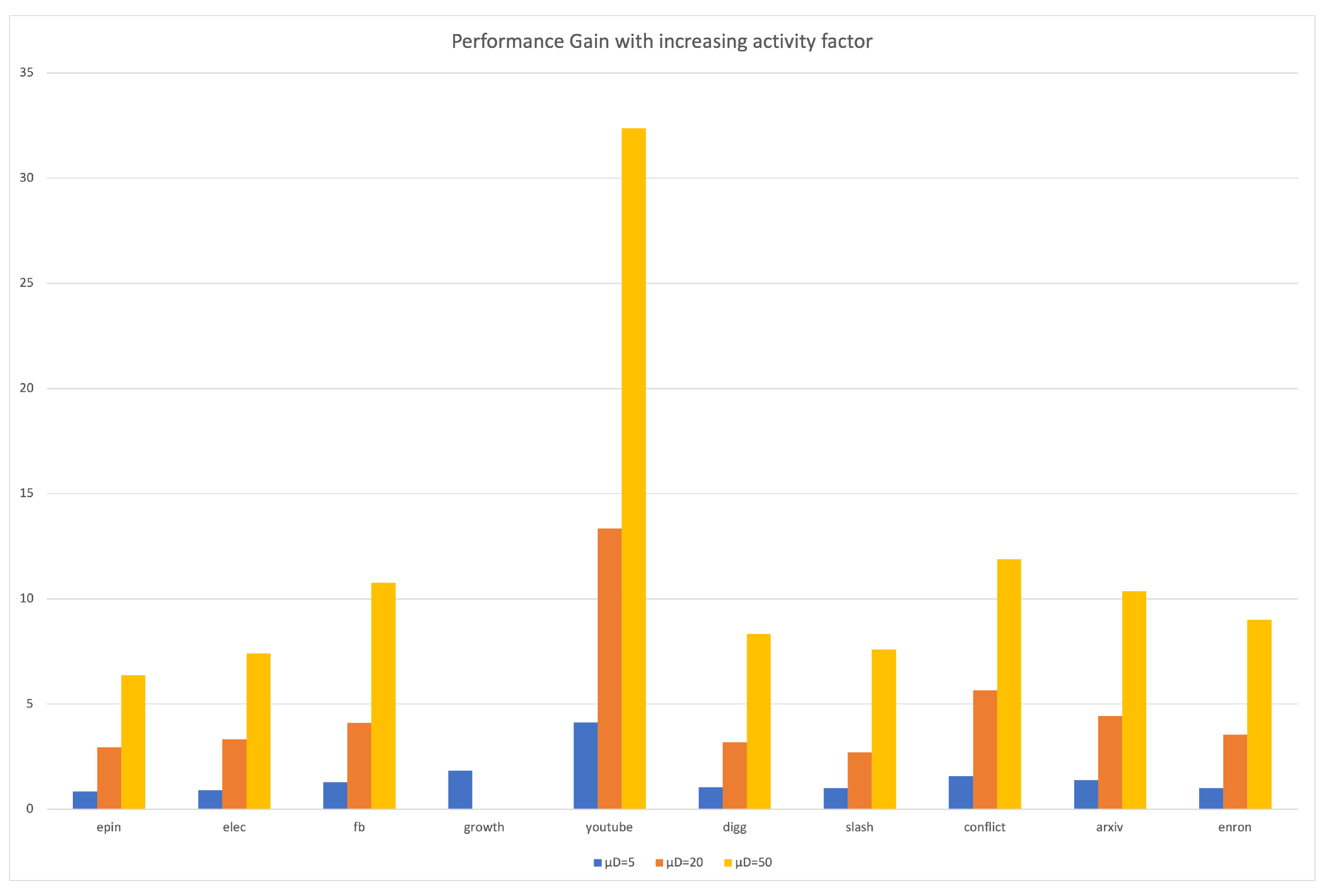
Experimentally, it is demonstrated that as the contiguous time intervals that allow travel on edges in temporal graphs become larger, our $ITG$ shortest path algorithm shows increasing performance gains over the algorithm by Wu et al. [15] running on the same temporal graph expressed as a $CSG$.

Our main contributions are as follows:

• We develop a polynomial time algorithm to find the shortest paths in an $ITG$. To the best of our knowledge, no such algorithm is presently available in the literature.
• We provide the complexity analysis of our shortest path algorithm.
• We benchmark our algorithm for $ITG$s against that of Wu et al. [15] for finding the shortest paths in $CSG$s. Experimentally, we show that as the activity factor in a temporal graph increases due to large contiguous travel intervals, our algorithm shows increasing performance gains over that of Wu et al. [15] on equivalent temporal graphs expressed as $CSG$s. Using synthetic datasets, we show that our algorithm for $ITG$s obtains a speedup of up to $32.5$ relative to the state-of-the-art algorithm for $CSG$s.

2. Problem Description

Definitions

Definition 1 

(Contact sequence temporal graph). In a contact sequence temporal graph $G=(V,E)$, each edge $e\in E$ is a tuple $(u,v,t,\lambda )$, where t is a permissible departure time for travel from u to v along the edge e and λ is the amount of time it takes to travel on edge e from u to v when departing at time t. Thus, v is reached at time $t+\lambda$. If there are m time instances when departures from u to v are permissible, there will be m such temporal edges $[(u,v,t_1,{\lambda }_1);(u,v,t_2,{\lambda }_2)\dots ;(u,v,t_m,{\lambda }_m)]$. m is the amount of activity on the connection $(u,v)$.

Definition 2 

(Interval temporal graphs). In an interval temporal graph $G=(V,E)$, each edge $e\in E$ is represented by a tuple $(u,v,intvls)$. This tuple represents a connection from u to v. $intvls$ is a time-ordered non-overlapping vector of tuples $[(s_1,c_1,{\lambda }_1);(s_2,c_2,{\lambda }_2);\dots ;(s_n,c_n,{\lambda }_n)]$. The ith interval starts at time $s_i$ and closes (ends) at time $c_i$; ${\lambda }_i$ is the time it takes to traverse the edge when departing u at a time t if $[s_i\le t\le c_i]$ (v is reached at time $t+{\lambda }_i$). The intervals are in ascending order of start times $s_i$, and collectively, they define the permissible departure times from u.

The permissible travel intervals for any edge of an $ITG$ (Definition 2) can be adjusted such that for any two consecutive intervals $[(s_i,c_i,{\lambda }_i);(s_{i+1},c_{i+1},{\lambda }_{i+1})]$ we have $(c_i+{\lambda }_i\le s_{i+1}+{\lambda }_{i+1})$. This transformation is explained in Jain and Sahni [18]. In this paper, we assume that the intervals associated with each edge of an $ITG$ satisfy this constraint.

As is evident from Figure 3 and Figure 4, a given temporal graph may need a much larger number of edges to be expressed as a $CSG$ versus an $ITG$. This is especially true when the graph has large contiguous travel intervals on the edges. Jain et al. [18] demonstrated that several temporal path and walk problems on $CSG$s may be polynomial in the size of the input graph but NP-hard for the equivalent $ITG$ graph.

Figure 3. Interval temporal graph with large intervals.

Figure 4. High-activity contact sequence graph.

Definition 3 

(Temporal paths and walks). A $path$ (equivalently, valid path, feasible path, temporal path or time-respecting path), $p=\{u_1,t_1,u_2,t_2,...,u_k\}$, in a temporal graph is an alternating sequence of vertices and departure times from those vertices starting from a source vertex $u_1$ to a destination vertex $u_k$ such that no vertex appears more than once in this sequence. $t_i$ is a permissible departure time from $u_i$ to $u_{i+1}$ and $(t_i+{\lambda }_i)\le t_{i+1}$, $1\le i<k$. $(t_i+{\lambda }_i)$ is the arrival time at $u_{i+1}$ when departing $u_i$ at $t_i$, $1\le i<k$. For path p, $u_1$ is the source or start vertex and $u_k$ is the destination vertex. The number of hops is $k-1$. When vertices are permitted to repeat in p, p is a $walk$. Note that every path is also a walk but some walks are not paths.

Definition 4 

(Shortest paths). A shortest path p in a temporal graph is a feasible temporal path from a start vertex $u_1$ to a destination vertex $u_k$ with minimum length, where the length, $len\left(p\right)$, of a path p is the sum of the travel times ${\lambda }_i$ on the edges $e_i$ on this path.

$$len\left(p\right)=\sum _{i=1}^{k-1}{\lambda }_i$$

(1)

By contrast, a fastest path from $u_1$ to $u_k$ is a temporal path that minimizes the difference between the arrival time at $u_k$ and the departure time from $u_1$. Such a path accounts for wait times at all intermediate vertices. Algorithms for fastest paths in interval and contact sequence temporal graphs may be found in [15,16,17,21]. Shortest paths are of interest in applications where there is a cost associated with traveling on an edge but no cost associated with waiting at a vertex. For example, the fuel cost depends on the sum of the ${\lambda }_i$s and is independent of the wait times at the vertices.

It is to be noted that the shortest path p from vertex $u_1$ to $u_k$ in a temporal graph is also the shortest walk from $u_1$ to $u_k$. To see this, assume there is a walk w of shorter length. The walk w can be converted to a path $p^{\prime }$ from $u_1$ to $u_k$ by removing all of its cycles. Since edge travel times are non-negative, $len\left(p^{\prime }\right)\le len\left(w\right)<len\left(p\right)$, contradicting the fact that p is a shortest path from $u_1$ to $u_k$.

3. Shortest Paths

We need to find the shortest paths p from a start vertex s to all possible destination vertices $u_k$ in a given $ITG$.

3.1. Dominance Criteria

Let $p1$ and $p2$ be two paths from the start vertex s to the same end vertex v. We say that $p1$ dominates $p2$ iff every valid extension of $p2$ is also a valid extension of $p1$ and has the same or smaller length. A valid extension of a path p from s to v is a valid path $p^{\prime }$ from s to $v^{\prime }$, such that $p^{\prime }$ goes through v and is the same as p from s to v. 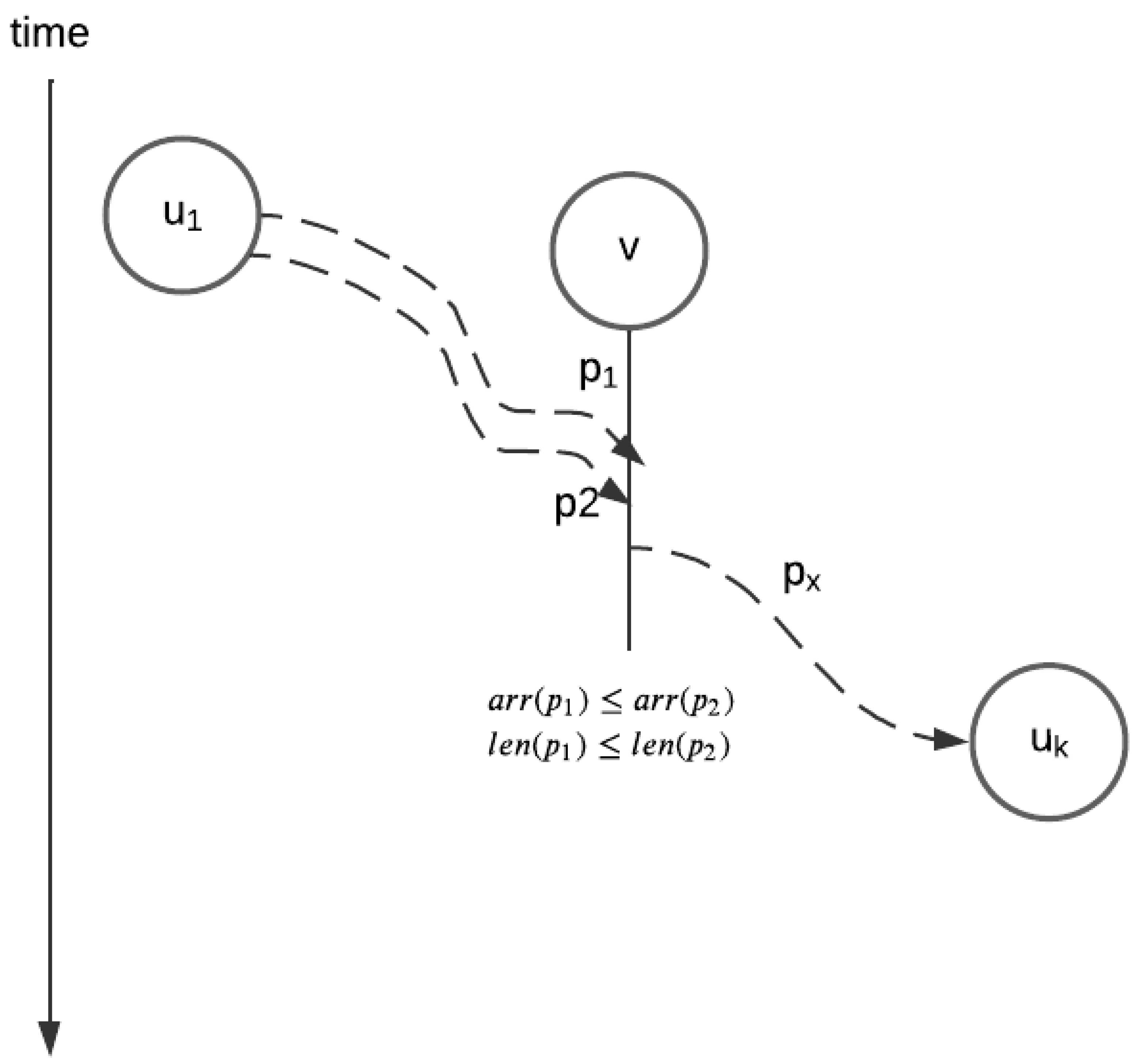Let the arrival time and length of a path p from s (to its end vertex) be denoted by $arr\left(p\right)$ and $len\left(p\right)$, respectively. It is easy to see that when Equation (2) is true, $p1$ dominates $p2$ (see Figure 5).

$$\begin{array}{cc}\hfill arr\left(p1\right)& \le arr\left(p2\right)\hfill \\ \hfill len\left(p1\right)& \le len\left(p2\right)\hfill \end{array}$$

(2)

Figure 5. $p1$ dominates $p2$.

When the arrival times and lengths of the paths $p1$ and $p2$ are as in Equation (3), then neither of the paths dominates the other. When neither path dominates the other, we say that $p1$ and $p2$ are pairwise non-dominant.

$$\begin{array}{cc}\hfill arr\left(p1\right)& <arr\left(p2\right)\hfill \\ \hfill len\left(p1\right)& >len\left(p2\right)\hfill \end{array}$$

(3)

3.2. Algorithm

We propose a hop-by-hop algorithm to determine a shortest path from a start vertex s to all possible destinations $u_k$ in an $ITG$. At every hop count k, we construct a list of non-dominated paths from s to every reachable vertex v by extending the list of such paths for hop count $k-1$. The algorithm terminates after a maximum of $n-1$ hops, where n is the total number of vertices in the $ITG$ or when no new non-dominated paths are discovered in a given hop.

3.3. Overview

Let $P(v,k)$ be the list of pairwise non-dominant r-hop paths $(t,l)$ from s to v that arrive at v at time t and have length l, $r\le k$; the paths are in increasing order of t (equivalently, decreasing order of l). Let $P_{new}(v,k)$ be the list of non-dominated k-hop paths from s to v. A high-level description of our shortest paths algorithm can be found in Algorithm 1.

The lists $P(v,0)$ and $P_{new}(v,0)$ are initialized in lines 1 and 2 to be lists of 0-hop paths from s to v. The $(k-1)$-hop paths in $P_{new}(u,k-1)$ are extended to k-hop paths by adding an outgoing edge $(u,v)$ in lines 8 and 10. Line 8 considers one edge extensions that use the interval $(i.st,i.c)$ for the case $t<i.st$. Of the possible extensions using this interval, the one that departs u at time $i.st$ dominates the others and so only this one is added to $P_{new}(v,k)$. Line 10 considers the remaining case for a legitimate extension, $i.st\le t\le i.c$. Again, only the single non-dominated extension is added to $P_{new}(v,k)$. Line 13 removes dominated paths from $P_{new}(v,k)$. In Line 14, the paths in $P(v,k-1)$ and $P_{new}(v,k)$ are merged to obtain $P(v,k)$ (recall that $P(v,k)$ is to contain only non-dominated paths). Additionally, paths in $P_{new}(v,k)$ that are dominated by a path in $P(v,k-1)$ are eliminated from $P_{new}(v,k)$.

Algorithm 1 Shortest Paths Pseudocode

1: $P(s,0)\leftarrow \left\{\right(0,0\left)\right\},shrtstP\left(s\right)=(0,0)$;$\forall v\ne s,P(v,0)\leftarrow ⌀,shrtstP\left(v\right)=⌀$ 2: $P_{new}(s,0)\leftarrow \left\{(0,0)\right\}$;$\forall v\ne s,P_{new}(v,0)\leftarrow ⌀$ 3: for  $k=1,\dots ,n-1$  do 4:       $\forall v,P_{new}(v,k)=⌀$ 5:       for every edge $(u,v)|P_{new}(u,k-1)\ne ⌀$ do 6:            for all $(t,l)\in P_{new}(u,k-1)$ do 7:                   $\forall i\in (u,v)|t<i.st$ add $(t^{\prime },l^{\prime })=$ 8:                            $(i.st+i.\lambda ,l+i.\lambda )$ to $P_{new}(v,k)$ 9:                   If there is an i, such that $i.st\le t\le i.c$, add 10:                  $(t^{\prime },l^{\prime })=(t+i.\lambda ,l+i.\lambda )$ to $P_{new}(v,k)$ 11:          end for 12:      end for 13:      $\forall v$, eliminate dominated paths from $P_{new}(v,k)$ 14:      $\forall v$, merge $P_{new}(v,k)$ and $P(v,k-1)$ to get $P(v,k)$ eliminating dominated paths from $P(v,k-1)$ as well as paths in $P_{new}(v,k)$ that are dominated by paths in $P(v,k-1)$ 15:      $\forall v|P_{new}(v,k)\ne ⌀$, $shrtstP\left(v\right)=P(v,k).shrtst\left(\right)$ 16:      If $\forall v,P_{new}(v,k)=⌀$ terminate! 17: end for 18: return shrtstP[]

3.4. Pseudocode Example Walk-Through

We will walk through the pseudocode in Algorithm 1 with an example graph of Figure 6. We are to find the shortest paths from s to all destination vertices $v\in \{a,b,c,d\}$ in Figure 6. The lists $P(v,0)$ and $P_{new}(v,0)$ are initialized as ⌀ in lines 1 and 2 for $v\in \{a,b,c,d\}$ as 0-hop paths. $P(s,0)$ and $P_{new}(s,0)$ are initialized as $\left\{\right(0,0\left)\right\}$. $shrtstP\left(s\right)=(0,0)$

Figure 6. Shortest paths in $ITG$ example.

• In hop 1, $k=1$. The condition in line 5 evaluates to true only for the edge $(s,a)$. Therefore, lines 6 to 11 add two new paths to $P_{new}(a,1)$ as $\left\{\right(2,1),(4,1\left)\right\}$, extending $(0,0)$ along the two available intervals on edge $(s,a)$. Line 13 eliminates the path $(4,1)$ from $P_{new}(a,1)$ as it is dominated by the path $(2,1)$ as per Equation (2). Merging $P_{new}(a,1)$ with $P(a,0)=⌀$ in line 14 gives $P(a,1)=P_{new}(a,1)=\left\{(2,1)\right\}$. $shrtstP\left(a\right)=(2,1)$
• In hop 2, $k=2$. Line 5 evaluates to true for edges $(a,b)$ and $(a,c)$ since $P_{new}(a,1)=\left\{(2,1)\right\}$. Hence, $(2,1)$ is extended along each of these edges in lines 6 to 11.

  (a)

  Extending $(2,1)$ along the two intervals on edge $(a,b)$ gives $P_{new}(b,2)=\{(3,2),(17,5)\}$

  (b)

  Extending $(2,1)$ along the two intervals on edge $(a,c)$ gives $P_{new}(c,2)=\{(6,3),(10,2)\}$

  Line 13 eliminates the dominated path $(17,5)$ from $P_{new}(b,2)$, whereas none of the paths are dominated in $P_{new}(c,2)$. Lists $P_{new}(b,2)$ and $P_{new}(c,2)$ are merged with $P(b,1)=⌀$ and $P(c,1)=⌀$, respectively, in line 14. Therefore, at the end of this iteration, $P_{new}(b,2)=P(b,2)=(3,2)$ and $P_{new}(c,2)=P(c,2)=\{(6,3),(10,2)\}$.
  $shrtstP\left(b\right)=(3,2);shrtstP\left(c\right)=(10,2)$.
• In hop 3, $k=3$. We have $P_{new}(b,2)$ and $P_{new}(c,2)$ as non-empty. Therefore, line 5 evaluates to true for edges $(b,d)$ and $(c,d)$.

  (a)

  Extension of paths in $P_{new}(b,2)=\left\{(3,2)\right\}$ along the intervals on edge $(b,d)$ gives $P_{new}(d,3)=\left\{(5,4)\right\}$.

  (b)

  Extension of paths in $P_{new}(c,2)=\{(6,3),(10,2)\}$ along the intervals on edge $(c,d)$ appends $\left\{\right(11,4),(11,3\left)\right\}$ to $P_{new}(d,3)$. Therefore, $P_{new}(d,3)=\{(5,4),(11,4),(11,3)\}$.

  Line 13 eliminates the dominated paths from $P_{new}(d,3)$. Therefore, the paths surviving are $P_{new}(d,3)=\{(5,4),\left(11.3\right)\}$. After merging $P_{new}(d,3)$ with $P(d,2)=⌀$ in line 14 we obtain, $P_{new}(d,3)=P(d,3)=\{(5,4),(11,3)\}$. $shrtstP\left(d\right)=(11,3)$.

Line 5 does not evaluate to true for any other edges when $k=4$, as even though $P_{new}(d,3)$ is non-empty, there are no outgoing edges from d. Therefore, the algorithm terminates. The shortest paths to each of the vertices $(s,a,b,c,d)$ are available in the array $shrtstP$.

3.5. Detailed Algorithm

Algorithm 2 is a refinement of Algorithm 1 that provides a greater level of detail.

The function $nextI\left(\right(u,v),(t,l\left)\right)$ (line 12 of Algorithm 2) finds the earliest possible departure time $fstout$ and corresponding interval $i_F$ on the edge $(u,v)$. If t is in the interval $(i_F.st,i_F.c)$, $fstout$ is the same as t, otherwise it is $i_F.st$. The lists of paths $(t,l)$ arriving at a vertex are always kept in increasing order of t. In a list of non-dominated paths, the increasing order of t is the same as the decreasing order of l due to the dominance criteria of Section 3.1. In line 17, $prpendDom(P_{new}^{″}(v,k),(t^{\prime },l^{\prime }))$ prepends extended path $(t^{\prime },l^{\prime })$ to the list $P_{new}^{″}(v,k)$ since paths $(t,l)$ from the predecessor vertex u are extended in decreasing order of t. After prepending $(t^{\prime },l^{\prime })$ to $P_{new}^{″}(v,k)$, $prependDom$ eliminates any subsequent paths in the list that $(t^{\prime },l^{\prime })$ dominates.

In lines 11 to 24, every $(t,l)$ is extended using an outgoing edge $(u,v)$ and the earliest possible departure time $fstout$ ($\ge t$) from u. Then, $(t,l)$ is also extended at $i.st$ for every subsequent interval i on $(u,v)$, such that $i.st<prev\left(fstout\right)$, where $prev\left(fstout\right)$ is the extension time of a previously examined path $(t_p,l_p)$ at u. This is because extension of $(t,l)$ would be dominated by the extension of $(t_p,l_p)$ if it starts at $t_x\ge prev\left(fstout\right)$ with the same travel time ${\lambda }_x$ since $l_p<l$.

In line 25, the list of extensions of all paths from u to v is merged with any other such list from a different incoming edge $(u^{\prime },v)$ in the current hop, retaining only non-dominated paths. The resulting $P_{new}^{\prime }(v,k)$ is added to $nxtPLists$, which maintains all such lists obtained at every vertex v in hop k.

Algorithm 2 Shortest Paths Detailed Algorithm

1: Initialize $P(v,0)\leftarrow NULL$, $\forall v\ne s$; $P(s,0)\leftarrow (0,0)$ 2: Initialize $newPLists$ as empty list. $P_{new}(s,0)\leftarrow (0,0)$. 3: $\forall v\ne s$, $shrtstP\left[v\right]\leftarrow (\infty ,\infty )$; $shrtstP\left[s\right]\leftarrow (0,0)$ 4: Add $[s,P_{new}(s,0)]$ to $newPLists$ 5: Initialize $k\leftarrow 0$; $newPaths\leftarrow 1$ 6: while $k<n-1$ and $newPaths>0$ do 7:     $newPaths\leftarrow 0$;$k++$ 8:     for all u in $newPLists$ do 9:         for all neighbors v of u do 10:              Initialize $prevPath\left(fstout\right)\leftarrow \infty$ 11:              for all $(t,l)\in P_{new}(u,k-1)$ in dec order of t do 12:                   $(i_F,fstout)\leftarrow nextI((u,v),(t,l))$ 13:                   if $fstout\ge prevPath\left(fstout\right)$ then 14:                       continue 15:                   end if 16:                   $(t^{\prime },l^{\prime })\leftarrow (fstout+i_F.\lambda ,l+i_F.\lambda )$ 17:                   prpendDom($P_{new}^{″}(v,k),(t^{\prime },l^{\prime })$) 18:                   for $\left(\right\{i_x\in (u,v)|$ 19:                   $i_F.c\le i_x.st<prevPath\left(fstout\right)\left\}\right)$ do 20:                       $(t^{\prime },l^{\prime })\leftarrow (i_x.st+i_x.\lambda ,l+i_x.\lambda )$ 21:                       insrtDom($P_{new}^{″}(v,k),(t^{\prime },l^{\prime })$) 22:                   end for 23:                   $prevPath\left(fstout\right)\leftarrow fstout$ 24:               end for 25:               addOrmerge($[v,P_{new}^{″}(v,k)]$,$nxtPLists$) 26:         end for 27:     end for 28:     for all u in $nxtPLists$ do 29:         $(P(u,k),P_{new}(u,k))\leftarrow$ 30:          $EvalAndMerge(P(u,k-1),P_{new}^{\prime }(u,k))$ 31:         $shrtstP\left[u\right]\leftarrow P(u,k).last\left(\right)$ 32:         if $P_{new}(u,k).size\left(\right)>0$ then 33:            $newPaths++$ 34:         end if 35:     end for 36:     $newPLists\leftarrow nxtPLists$ 37:     $nxtPLists.clear\left(\right)$ 38: end while 39: return $shrtstP$

Finally, in line 30, all $P_{new}^{\prime }(u,k)$ at every vertex u available in $nxtPLists$, are evaluated against their respective $P(u,k-1)$ to obtain the non-dominated paths in hops 1 through k as $P(u,k)$ and the new paths in current hop as $P_{new}(u,k)$.

The algorithm continues until the terminating conditions are met.

Theorem 1. 

Algorithm 2 finds the shortest paths from the start vertex s to all reachable vertices v.

Proof. 

In an n-vertex temporal graph, a shortest path from a start vertex s to any destination vertex v is a non-dominated path with $\le n-1$ hops. In Algorithm 2, we examine all non-dominated paths starting from s and keep a record of the shortest path discovered in line 31. Due to our scheme of resolving the ties described in Section 3.2, any walks with cycles are eliminated as these are dominated by paths that have no cycles and have fewer hops. Therefore, the shortest path obtained is a shortest valid path with no cycles. □

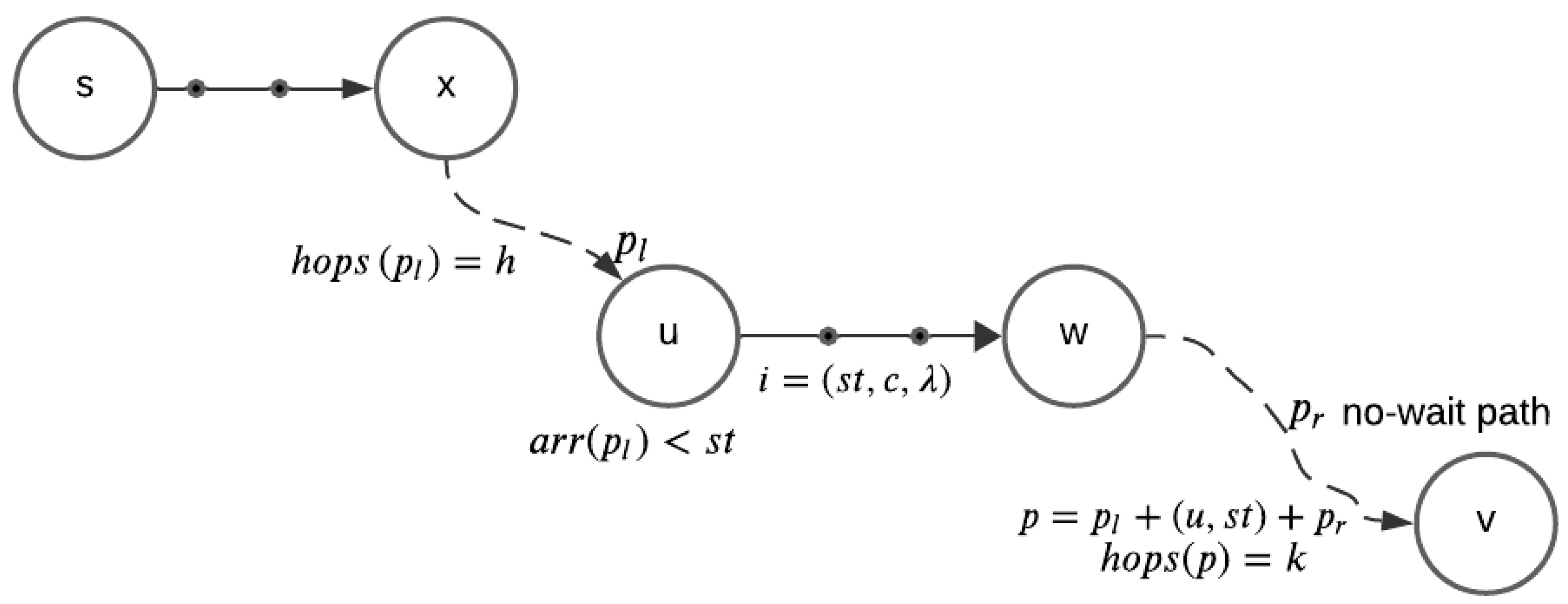
3.6. Complexity Analysis

We may associate a label $(eid,st,h)$ with each path $p\in P(v,k)$, $v\ne s$, and $k>0$, where $eid$ is the id of the last edge, $(u,w)$, in p with a departure time that is the start, $st$, of some travel interval of $(u,w)$ and h is the number of hops in the path p from s to u. Note that every $p\in P(v,k)$ has such a $(u,w)$ as the departure time for the first edge $(s,x)$ of p is the start of some interval of $(s,x)$ and the number of edges in p is finite. Let $p_l$ be the portion of p from s to u and $p_r$ that from u to v (see Figure 7). From the way our algorithm works, it follows that $p_l$ is an h-hop path in $P(u,h)$. Further, since the departure time for no edge in $p_r$ is a start time of a travel interval for that edge (except $st$ on $(u,w)$), $p_r$ encounters no wait at intermediate vertices and the length, $len\left(p_r\right)$, (i.e., sum of the edge travel times) of $p_r$ is the same as its duration (arrival time at v - departure time from u).

Figure 7. A $p\in P(v,k)$ and its label $(eid,st,h)$.

Theorem 2. 

No $P(v,k)$ has two paths with the same label.

Proof. 

Assume there is a $P(v,k)$ that has two paths $p1$ and $p2$ with the same label $(eid,st,h)$. We shall show that this assumption leads to a contradiction and so must be false. Note that $p1$ and $p2$ are pairwise non-dominant.

• Case $h=0$. Now, $p{1}_l$ and $p{2}_l$ are empty. Thus, $len\left(p1\right)=len\left(p{1}_r\right)=arr\left(p1\right)-st$ and $len\left(p2\right)=arr\left(p2\right)-st$. When $len\left(p1\right)<len\left(p2\right)$, we have $arr\left(p1\right)<arr\left(p2\right)$. Thus, $p1$ dominates $p2$, which contradicts the fact that $p1$ and $p2$ are pairwise non-dominant. A contradiction is similarly obtained for the cases $len\left(p1\right)=len\left(p2\right)$ and $len\left(p1\right)>len\left(p2\right)$.
• Case $h>0$. Now, $p{1}_l$ and $p{2}_l$ are h-hop paths from s to the same vertex u. The first edge of $p{1}_r$ and $p{2}_r$ is $(u,w)$ and both these paths start from u at time $st$. Thus,

  $$arr\left(p1\right)=st+len\left(p{1}_r\right)$$

  (4)

  $$arr\left(p2\right)=st+len\left(p{2}_r\right)$$

  (5)

  $$len\left(p1\right)=len\left(p{1}_l\right)+len\left(p{1}_r\right)$$

  (6)

  $$len\left(p2\right)=len\left(p{2}_l\right)+len\left(p{2}_r\right)$$

  (7)

  (a)

  Case $len\left(p{1}_1\right)=len\left(p{2}_l\right)$. Now, $p{1}_l$ and $p{2}_l$ must be the same path as, otherwise, one dominates the other, which is not possible as both are in $P(u,r)$. If $arr\left(p1\right)<arr\left(p2\right)$, then $len\left(p{1}_r\right)<len\left(p{2}_r\right)$ (Equations (4) and (5)). Thus, $len\left(p1\right)<len\left(p_2\right)$ (Equations (6) and (7)). Hence, $p1$ dominates $p2$, a contradiction. A similar proof shows that when $arr\left(p1\right)>arr\left(p2\right)$, we obtain the contradiction that $p2$ dominates $p1$.

  (b)

  Case $len\left(p{1}_l\right)<len\left(p{2}_l\right)$. Let $p3$ be the s to v path obtained by concatenating $p{1}_l$ and $p{2}_r$. Note that $p3$ is a k-hop time-respecting path with $arr\left(p3\right)=arr\left(p2\right)$ and $len\left(p3\right)=len\left(p{1}_l\right)+len\left(p{2}_r\right)<len\left(p2\right)$ (Equation (7)). Hence, $p3$ dominates $p2$. Thus, either $p3$ or a path $p4$ that dominates both $p2$ and $p3$ must be in $P(v,k)$. This means that $p2$ cannot be in $P(v,k)$.

  (c)

  Case $len\left(p{1}_l\right)>len\left(p{2}_l\right)$. This is similar to the previous case.

□

Theorem 3. 

No $P_{new}(v,k)$ has two paths with the same label.

Proof. 

This is similar to that of Theorem 2. □

The number of distinct path labels $(eid,st,h)$ is at most $i\ast n$, where i is the total number of travel intervals across all edges of the temporal graph. From Theorems 2 and 3, it follows that $\left|P\right(v,k\left)\right|\le in$ and $|P_{new}(v,k)|\le in$ for all v and k.

For each value of k, $k>0$, the at most $in$ paths in $P_{new}(u,k-1)$ are considered in increasing order of length (equivalently, decreasing order of arrival time at u) and extended by one hop using an out edge from u. When extending using the edge $(u,v)$ for each of these up to $in$ paths, a binary search is performed over the travel intervals of this edge to determine the first interval for a valid extension (line 12 of Algorithm 2). The remaining (larger start time) intervals are then examined serially until the first interval that has already been used for the extension of a previously considered path in $P(v,k-1)$ is encountered. Let $\delta$ be the maximum number of travel intervals on any edge. We see that $O\left(in\log \delta \right)$ time is spent performing the binary searches for the up to $in$ paths and $O(\delta +in)$ time in examining the remaining intervals. The total time to process $(u,v)$ is therefore $O\left(in\log \delta \right)$ (note that $\delta \le i$). The number of k-hop paths generated by extending the paths in $P_{new}(u,k-1)$ using the edge $(u,v)$ is $O(in+\delta )=O\left(in\right)$.

To compute $P_{new}(v,k)$, we need to compute a list of extensions of the paths in $P_{new}(u,k-1)$ for all u such that $(u,v)$ is an edge of the temporal graph and merge these lists together, eliminating dominated paths. There are at most $indegree\left(v\right)$ such path lists to be merged. Each of these has $O\left(in\right)$ paths and takes $O\left(in\log \delta \right)$ time to compute. The time needed to compute all of these lists is therefore $O(in\log \delta \ast indegree(v\left)\right)$. Pairwise merging these path lists takes $O(in\ast indegree(v\left)\right)$ time (note that during the pairwise merge of two path lists, dominated paths are eliminated, so, from Theorem 3, it follows that the list size remains $O\left(in\right)$; two ordered path lists may be merged in linear time eliminating dominated paths). An alternative to pairwise merging of the path lists is to merge the $indegree\left(v\right)$ lists simultaneously using a loser tree. This reduces the merging time to $O(in\ast \log indegree(v\left)\right)$. Regardless, the total time needed to compute $P_{new}(v,k)$ is $O(in\log \delta \ast indegree(v\left)\right)$. Hence, for any k, all $P_{new}(v,k)$s may be computed in $O\left(ine\log \delta \right)$ time, where $e=\sum indegree\left(v\right)$ is the number of edges in the temporal graph.

For any k and v, $P_{new}(v,k)$ may be merged with $P(v,k-1)$, eliminating dominated pairs from both lists in $O\left(in\right)$ time as both lists are ordered by arrival time and of size $O\left(in\right)$ (Theorems 2 and 3). Thus, the overall time taken by Algorithm 2 for each k is $O\left(ine\log \delta \right)$ and the time over all ks is $O\left(i{n}^{2}e\log \delta \right)$, which is polynomial in the number of inputs.

4. Experimental Results

In this section, we compare the relative performance of Algorithm 2 for $ITG$s with the shortest path algorithm of Wu et al. [15] running on equivalent $CSG$s. Our experimental platform was an Intel Core i9-7900X CPU with a 3.30 GHz processor and 64 GB RAM. The C++ code for the shortest path algorithm of Wu et al. was obtained from the authors of [17]. Our algorithm was also coded in C++. The codes were compiled using the g++ ver. 7.5.0 compiler with option O2. The datasets used for comparison of the relative performance are described in Section 4.1.

4.1. Datasets

Ref. [15] uses datasets from the Koblenz network [22]. These datasets have an (edge) activity that ranges from a low of about 1 to a high of about 3.67, which is rather low. Further, all $\lambda$ values are 1. The Koblenz datasets are described in Table 1. These datasets are in the form of $CSG$s where every allowed travel from one vertex to another is a single time instance. To benchmark our algorithm against the shortest paths algorithm of [15] on a wide variety of temporal graphs, we prepared synthetic datasets using the Koblenz graphs as follows:

Table 1. Koblenz graph statistics.

Dataset	$\left|\mathit{V}\right|$	$|{\mathit{E}}_{\mathit{s}}|$	$\mathit{cs}-\mathit{Edges}$	Activity
epin	$131.8$ K	$840.8$ K	$841.3$ K	1
elec	7119	$103.6$ K	$103.6$ K	1
fb	$63.7$ K	817 K	817 K	1
growth	$1870.7$ K	39,953 K	39,953 K	1
youtube	3223 K	9375 K	9375 K	1
digg	$30.3$ K	$85.2$ K	$87.6$ K	1.02
slash	51 K	$130.3$ K	$140.7$ K	1.07
conflict	118 K	$2027.8$ K	$2917.7$ K	1.43
arxiv	28 K	3148 K	4596 K	1.45
enron	87,274	$320.1$ K	1148 K	3.58

• Obtain the underlying static graph from each Koblenz $CSG$. For this, we replaced each temporal edge $(u,v,t,\lambda )$ by the static edge $(u,v)$ and eliminated duplicate static edges.
• Represent the static graph obtained in the previous step as an array adjacency list.
• On every static edge, we randomly add temporal intervals. The temporal intervals are added using three random variables, number of allowed travel intervals I, duration of each interval D and the travel time on each interval T. Values are assigned to each of these random variables using a normal distribution around three parameters $({\mu }_I,{\mu }_D,{\mu }_T)$, respectively. These parameters are the mean values for the normal distribution defining the three random variables $(I,D,T)$, respectively.

We increase the activity factor in the temporal graph by gradually increasing the value of the parameter ${\mu }_D$. For each $ITG$ obtained using the method described above, we obtain an equivalent $CSG$ to benchmark against the shortest path algorithm of [15]. The synthetic datasets obtained as outlined above are described in Table 2. For the $growth$ dataset, the number of contact sequence edges is too large to accommodate in a 32-$bit$ integer for ${\mu }_D=20$ and ${\mu }_D=50$. Therefore, it was infeasible to build a corresponding $CSG$ and run the algorithm from [15] on it. However, we could still run our algorithm on the $ITG$ representation; the run times were quite reasonable. Table 3 reports the size of each of the synthetic datasets on disk. As we increase the activity factor of the temporal graph by increasing the ${\mu }_D$ parameter, the size of the $CSG$ representation of the graph increases significantly. For example, for the $enron$ dataset, the size of the $ITG$ is $19.5$ MB for ${\mu }_D=50$, as compared to $10.7$ GB for the $CSG$ representation of the same temporal graph, which is a ratio of approximately 563.

Table 2. Synthetic graphs’ statistics.

Graphs with ${\mathit{\mu }}_{\mathit{I}}=4,{\mathit{\mu }}_{\mathit{T}}=3$
Dataset	$\left|\mathit{V}\right|$	$|{\mathit{E}}_{\mathit{s}}|$	cs-Edges (${\mathit{\mu }}_{\mathit{D}}=\mathbf{5}$)	cs-Edges (${\mathit{\mu }}_{\mathit{D}}=\mathbf{20}$)	cs-Edges (${\mathit{\mu }}_{\mathit{D}}=\mathbf{50}$)
epin	131.8 K	840.8 K	17.8 M	65.2 M	160.6 M
elec	7119	103.6 K	2.2 M	8 M	19.8 M
fb	63.7 K	817 K	17.3 M	63.3 M	156 M
growth	1870.7 K	39,953 K	848.3 M	–	–
youtube	3.2 M	9.3 M	199 M	727.2 M	1.8B
digg	30.3 K	85.2 K	1.8 M	6.6 M	16.2 M
slash	51 K	130.3 K	2.7 M	10.1 M	24.9 M
conflict	118 K	2027.8 K	43.07 M	157.3 M	387.5 M
arxiv	28 K	3148 K	66.8 M	244.2 M	601.7 M
enron	87,274	320.1 K	6.8 M	24.8 M	61.1 M

Table 3. Synthetic graphs’ size on disk.

Dataset	ITG			CSG
	${\mathit{\mu }}_{\mathit{D}}=\mathbf{5}$	${\mathit{\mu }}_{\mathit{D}}=\mathbf{20}$	${\mathit{\mu }}_{\mathit{D}}=\mathbf{50}$	${\mathit{\mu }}_{\mathit{D}}=\mathbf{5}$	${\mathit{\mu }}_{\mathit{D}}=\mathbf{20}$	${\mathit{\mu }}_{\mathit{D}}=\mathbf{50}$
epin	$51.93$ MB	$51.94$ MB	$51.95$ MB	323 MB	$1.18$ GB	$2.9$ GB
elec	$6.2$ MB	$6.23$ MB	$6.23$ MB	$36.1$ MB	$132.2$ MB	$325.7$ MB
fb	$50.5$ MB	$50.5$ MB	$50.5$ MB	$314.8$ MB	$1.1$ GB	$2.83$ GB
growth	$2.55$ GB	$2.55$ GB	$2.55$ GB	$17.1$ GB	–	–
youtube	$609.3$ MB	$609.3$ MB	$609.3$ MB	$4.2$ GB	$15.5$ GB	$38.1$ GB
digg	$5.2$ MB	$5.2$ MB	$5.2$ MB	$31.4$ MB	$114.8$ MB	$282.6$ MB
slash	8 MB	8 MB	8 MB	49 M	$179.4$ MB	$442.2$ MB
conflict	126 MB	126 MB	126 MB	$794.5$ MB	$2.9$ GB	$7.1$ GB
arxiv	$191.8$ MB	$191.8$ MB	$191.8$ MB	$1.15$ GB	$4.21$ GB	$10.37$ GB
enron	$19.58$ MB	$19.58$ MB	$19.58$ MB	$1.18$ GB	$4.3$ GB	$10.7$ GB

4.2. Run Times

Since the $CSG$s are much larger in size as compared to the corresponding $ITG$s, the reading time (from disk) of the $CSG$ is also significantly larger. The comparison of the reading times for the graphs by our algorithm and by that of Wu et al. [15] is reported in Table 4. It is important to note that the reading times for our algorithm are almost the same for the different values of ${\mu }_D$. However, for the $CSG$s, the reading time increases proportionately to the increase in the activity factor. This is because the number of contact sequence edges also increases proportionately. The size of the $ITG$ representation, however, remains almost similar across different values of the parameter ${\mu }_D$.

Table 4. Synthetic graphs’ reading times in seconds.

Dataset	Ours on ITG			CSG Algorithm
	${\mathit{\mu }}_{\mathit{D}}=\mathbf{5}$	${\mathit{\mu }}_{\mathit{D}}=\mathbf{20}$	${\mathit{\mu }}_{\mathit{D}}=\mathbf{50}$	${\mathit{\mu }}_{\mathit{D}}=\mathbf{5}$	${\mathit{\mu }}_{\mathit{D}}=\mathbf{20}$	${\mathit{\mu }}_{\mathit{D}}=\mathbf{50}$
epin	$1.03$	$1.03$	$1.03$	$5.6$	$20.2$	$51.5$
elec	$0.14$	$0.13$	$0.12$	$0.69$	$2.5$	$6.1$
fb	1	$0.99$	$0.97$	$5.4$	$19.2$	$48.8$
growth	$50.5$	50	$50.5$	$271.65$	–	–
youtube	$11.8$	$12.09$	$12.34$	$64.4$	$235.1$	$578.1$
digg	$0.12$	$0.12$	$0.1$	$0.57$	$2.03$	$4.9$
slash	$0.17$	$0.16$	$0.16$	$0.88$	$3.1$	$7.6$
conflict	$2.4$	$2.4$	$2.4$	$13.3$	$48.9$	$121.7$
arxiv	$3.6$	$3.6$	$3.6$	$20.4$	$75.7$	$189.6$
enron	$0.4$	$0.39$	$0.39$	$2.1$	$7.7$	$19.2$

Comparisons of run times (excluding the time to read in the temporal graph) of the two algorithms on all the datasets are reported in Table 5. As expected, the run times of our algorithm remains almost the same across the different values of ${\mu }_D$. However, the run times of the algorithm in [15] increases proportionately to the increase in the value of ${\mu }_D$ and, hence, the number of contact sequence edges in the graph. Therefore, our algorithm shows increasing performance gains in run time and in memory consumption over that of Wu et al. [15] when the temporal graph has larger contiguous travel intervals. For our experiments, we limited the duration of the travel intervals to follow a normal distribution around ${\mu }_D=50$. This is because for much larger travel intervals, the algorithm of Wu et al. [15] runs out of memory due to the large number of contact sequence edges. In contrast, our algorithm comfortably handles large travel durations. One example of this is the $growth$ dataset for which our algorithm runs in reasonable times for the values of ${\mu }_D=20$ and ${\mu }_D=50$, whereas it is infeasible to represent the $CSG$ using 32-$bit$ integers for ${\mu }_D=20$.

Table 5. Synthetic graphs’ run time in seconds comparison.

Dataset	Ours on ITG			CSG Algorithm
	${\mathit{\mu }}_{\mathit{D}}=\mathbf{5}$	${\mathit{\mu }}_{\mathit{D}}=\mathbf{20}$	${\mathit{\mu }}_{\mathit{D}}=\mathbf{50}$	${\mathit{\mu }}_{\mathit{D}}=\mathbf{5}$	${\mathit{\mu }}_{\mathit{D}}=\mathbf{20}$	${\mathit{\mu }}_{\mathit{D}}=\mathbf{50}$
epin	$0.78$	$0.77$	$0.91$	$0.66$	$2.27$	$5.8$
elec	$0.044$	$0.045$	$0.05$	$0.04$	$0.15$	$0.37$
fb	$0.17$	$0.17$	$0.18$	$0.22$	$0.7$	$1.94$
growth	105	121	140	$192.8$	–	–
youtube	$0.63$	$0.63$	$0.63$	$2.6$	$8.4$	$20.4$
digg	$0.019$	$0.022$	$0.024$	$0.02$	$0.07$	$0.18$
slash	$0.1$	$0.1$	$0.11$	$0.1$	$0.27$	$0.76$
conflict	$0.57$	$0.53$	$0.64$	$0.9$	3	$7.6$
arxiv	$0.71$	$0.79$	$0.81$	$0.97$	$3.5$	$8.3$
enron	$0.08$	$0.09$	$0.1$	$0.08$	$0.32$	$0.9$

The performance gains obtained by our algorithm over that of Wu et al. [15] with increasing activity factor are shown in Figure 8.

Figure 8. Performance gains with increasing activity factor.

4.3. Memory Footprint

The ratio of the memory footprint of the algorithm of [15] to the memory footprint of our algorithm is similar to the ratio of the sizes of the corresponding temporal graph representation as $CSG$ and $ITG$, respectively. This is because both algorithms require the entire graph to be present in memory. As is evident from Table 3, this ratio increases significantly as the activity factor increases, going as high as 560 for our synthetic graphs.

5. Conclusions

We have developed a polynomial time shortest paths algorithm for the $ITG$ representation of temporal graphs. To the best of our knowledge, such an algorithm is not available in the literature. Our algorithm is suitable for temporal graphs with a high activity factor and large contiguous travel intervals. Our algorithm shows increasing performance gains over the known state-of-the-art shortest paths algorithm for $CSG$s as the activity factor on the temporal graphs increases. Using synthetic datasets, experimentally, we show that our algorithm for $ITG$s obtains a speedup of up to $32.5$ relative to the state-of-the-art algorithm for $CSG$s. For graphs with very large activity factors, the CSG algorithm is infeasible, while our algorithm can handle such datasets comfortably.