Improving the Generalization Abilities of Constructed Neural Networks with the Addition of Local Optimization Techniques

Abstract

Constructed neural networks with the assistance of grammatical evolution have been widely used in a series of classification and data-fitting problems recently. Application areas of this innovative machine learning technique include solving differential equations, autism screening, and measuring motor function in Parkinson’s disease. Although this technique has given excellent results, in many cases, it is trapped in local minimum and cannot perform satisfactorily in many problems. For this purpose, it is considered necessary to find techniques to avoid local minima, and one technique is the periodic application of local minimization techniques that will adjust the parameters of the constructed artificial neural network while maintaining the already existing architecture created by grammatical evolution. The periodic application of local minimization techniques has shown a significant reduction in both classification and data-fitting problems found in the relevant literature.

1. Introduction

Among the parametric machine learning models, one can find artificial neural networks (ANNs) [1,2], in which a set of parameters, also called weights, must be estimated in order for this model to adapt to classification or regression data. Neural networks have used problems derived from physics [3,4], problems involving differential equations [5], solar radiation prediction [6], agriculture problems [7], problems derived from chemistry [8,9], wind speed prediction [10], economics problems [11,12], problems related to medicine [13,14], etc. A common way to express a neural network is as a function $N(\overrightarrow{x},\overrightarrow{w})$. The vector $\overrightarrow{x}$ represents the input pattern to the neural network, and the vector $\overrightarrow{w}$ stands for the vector of parameters that must be computed. The set of parameters is calculated by minimizing the training error:

$$E\left(N\left(\overrightarrow{x},\overrightarrow{w}\right)\right)=\sum _{i=1}^M{\left(N\left({\overrightarrow{x}}_i,\overrightarrow{w}\right)-y_i\right)}^2$$

(1)

In Equation (1), the set $\left(\overrightarrow{x_i},y_i\right),i=1,\dots ,M$ stands for the train set. The values $y_i$ denote the target outputs for patterns $\overrightarrow{x_i}$. Recently, various methods have appeared that minimize this equation, such as the back propagation method [15], the RPROP method [16,17], the ADAM method [18], etc. Additionally, global optimization techniques were also used, such as the simulated annealing method [19], genetic algorithms [20], Particle Swarm Optimization (PSO) [21], Differential Evolution [22], Ant Colony Optimization [23], Gray Wolf Optimizer [24], Whale optimization [25], etc.

In many cases, especially when the data are large in volume or have a high number of features, significant times are observed during the process of training artificial neural networks. For this reason, techniques have been presented in recent years that exploit modern parallel computing structures for faster training of these machine learning models [26].

Another important aspect in artificial neural networks is the initialization of parameters. Various techniques have been proposed in this area, such as the usage of polynomial bases [27], initialization based on decision trees [28], usage of intervals [29], discriminant learning [30], etc. Also, recently, Chen et al. proposed a new weight initialization method [31].

Identifying the optimal architecture of an artificial neural network could be an extremely important factor to determine the generalization abilities of an artificial neural network. Networks with only a few neurons can be trained faster and may have good generalization abilities, but in many cases, the optimization method cannot escape from the local minima of the error function. Furthermore, networks with many neurons can have a significantly reduced training error but require a large computational time for their training and many times do not perform significantly when applied to data that are not present in the training set. In this direction, many researchers proposed various methods to discover the optimal architecture, such as the use of genetic algorithms [32,33], the Particle Swarm Optimization method [34], reinforcement learning [35], etc. Also, Islam et al. proposed a new adaptive merging and growing technique used to design the optimal structure of an artificial neural network [36].

Recently, a technique was presented that utilizes grammatical evolution [37] for the efficient construction of the architecture of an artificial neural network as well as the calculation of the optimal values of the parameters [38]. In this technique, the architecture of the neural network is identified. Also, the method performs feature selection, since only those features are selected which will reduce the training error. Using this technique, the number of features are reduced, leading to neural networks that are faster in response and have generalization abilities. The neural construction technique has been applied in a wide series of problems, such as the location of amide I bonds [39], solving differential equations [40], application in data collected for Parkinson’s disease [41], prediction of performance for higher education students [42], autism screening [43], etc. Software that implements the previously mentioned method can be downloaded freely from https://github.com/itsoulos/NNC (accessed on 28 September 2024) [44].

Although the neural network construction technique has been successfully used in a variety of applications and is able to identify the optimal structure of a neural network as well as find satisfactory values for the model parameters, it cannot avoid the local minima of the error function, which results in reduced performance. In this research paper, the periodic application of local optimization techniques is proposed in randomly selected artificial neural networks constructed by grammatical evolution. Local optimization does not alter the generated neural network structure but can more efficiently identify values of the network parameters with lower values of the training error. The current work was applied on many classification and data-fitting datasets, and it seems to reduce the test error obtained by the original neural construction technique.

The current paper have the following organization: Section 2 discusses the main aspects of the suggested method, Section 3 outlines the series of performed experiments, and Section 4 provides some conclusions and provided various guidelines for future research.

2. Method Description

This section initiates with a short description of the grammatical evolution method and continues with a detailed description of the proposed algorithm.

2.1. Grammatical Evolution

Grammatical evolution can be considered as a genetic algorithm with integer chromosomes. These chromosomes stand for a series of production rules in a grammar expressed in the Backus–Naur (BNF) form [45]. The method was used in data fitting [46,47], trigonometric problems [48], automatic composition of music [49], production of numeric constants with an arbitrary number of digits [50], video games [51,52], energy problems [53], combinatorial optimization [54], cryptography [55], the production of decision trees [56], electronics [57], Wikipedia taxonomies [58], economics [59], bioinformatics [60], robotics [61], etc. A BNF grammar is commonly defined as a set $G=\left(N,T,S,P\right)$. The following definitions hold for any BNF grammar:

• The set N contains the symbols denoted as non-terminal.
• The set T has the terminal symbols.
• The symbol $S\in N$ stands for the start symbol of the grammar.
• The set P has all the production rules of the underlying grammar. These rules are used to produce terminal symbols from non-terminal symbols, and they are in the form $A\to a$ or $A\to aB,A,B\in N,a\in T$.

The production algorithm starts from the symbol S and moves through a series of steps, producing valid programs by replacing non-terminal symbols with the right hand of the selected production rule. The selection of the production rules is performed in two steps:

• Read the the next element V from the processed chromosome.
• Select the production rule that will be applied using the equation: Rule = V mod $N_R$, where $N_R$ stands for the number of production rules that contains the current current non-terminal symbol.

The incorporated grammar for the neural construction method is outlined in Figure 1. The number in parentheses denotes the sequence number of each rule for every non-terminal symbol. The symbol n represents the number of features for the used dataset.

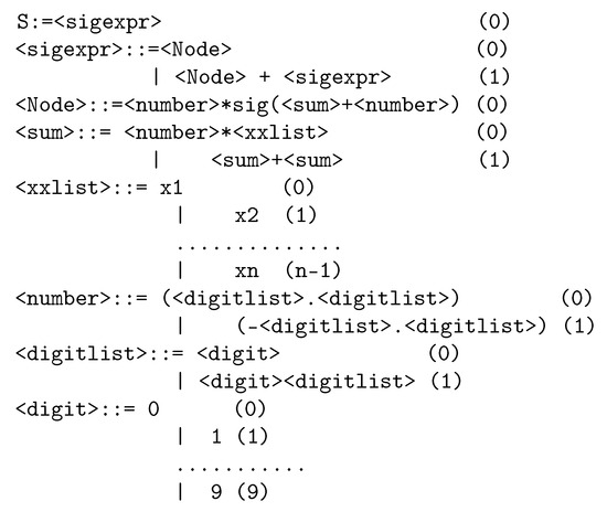
Figure 1. The grammar used by the neural construction method.

This grammar can produce artificial neural networks in the following form:

$$N\left(\overrightarrow{x},\overrightarrow{w}\right)=\sum _{i=1}^H{w}_{(n+2)i-(n+1)}\sigma \left(\sum _{j=1}^n{x}_j{w}_{(n+2)i-(n+1)+j}+w_{(n+2)i}\right)$$

(2)

The symbol H corresponds to the number of weights or processing units. The function $\sigma \left(x\right)$ denotes the sigmoid function, and it has the following definition:

$$\sigma \left(x\right)={\displaystyle \frac{1}{1+exp(-x)}}$$

(3)

The grammar of the present method can construct artificial neural networks with a hidden processing layer and with a variable number of computing units. This kind of architecture is sufficient to approach any problem, according to Hornik’s theorem [62], which states that an artificial neural network with a sufficient number of computing units and a processing level can approximate any function.

As an example, consider a problem with three inputs: $x_1,x_2,x_3$. An example neural network that can be constructed by the grammatical evolution procedure could be the following:

$$N\left(x\right)=2.1\mathrm{sig}\left(10.5x_2+9.2x_3+5.7\right)+3.2\mathrm{sig}\left(2.2x_1-4.3x_3+6.2\right)$$

(4)

The previously mentioned artificial neural network has two processing nodes, and not all inputs are necessarily connected to each processing node, since the grammatical evolution process may miss some connections.

2.2. The Proposed Algorithm

The steps of the current method are derived from the steps of the original neural network construction method with the addition of the periodical application of the local optimization algorithm as follows:

1.

Initialization step.

(a)

Set $k=0$ as the generation counter.

(b)

Set as $N_g$ the maximum number of generations and as $N_c$ the number of chromosomes.

(c)

Set as $p_s$ the selection rate and as $p_m$ the mutation rate of the genetic algorithm.

(d)

Set as $N_T$ the number of chromosomes that will be selected to apply the local search optimization method on them.

(e)

Set as $N_I$ the number of generations that should pass before the application of the suggested local optimization technique.

(f)

Set as F the range of values within which the local optimization method can vary the parameters of the neural network.

(g)

Perform a random initialization of the chromosomes $g_i,i=1,\dots ,N_c$ as sets of random integers.

2.

Fitness Calculation step.

(a)

For $i=1,\dots ,N_c$ do

i.

Produce the corresponding neural network $N_i\left(\overrightarrow{x},\overrightarrow{w_i}\right)$ for the chromosome $g_i$, The production is performed using the procedure of Section 2.1. The vector $\overrightarrow{w_i}$ denotes the set of parameters produced for the chromosome $g_i$.

ii.

Set as $f_i={\sum }_{j=1}^M{\left(N_i\left({\overrightarrow{x}}_j,\overrightarrow{w_i}\right)-y_j\right)}^2$ the fitness of chromosome i. The set $\left(\overrightarrow{x_j},y_j\right),j=1,\dots ,M$ represents the train set.

(b)

EndFor

3.

Genetic operations step.

(a)

Copy the best $\left(1-p_s\right)\times N_c$ chromosomes according to their fitness values to the next generation.

(b)

Apply the crossover procedure. This procedure creates $p_s\times N_c$ offsprings from the current population. Two chromosomes $(z,w)$ are selected through tournament selection for every created couple $\left(\tilde{z},\tilde{w}\right)$ of ofssprings. These offsprings are created using the one-point crossover procedure, which is demonstrated in Figure 2.

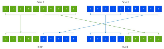Figure 2. An example of the method of one-point crossover used in the grammatical evolution procedure.

(c)

Apply the mutation procedure. During this procedure, a random number $r\in [0,1]$ is selected from uniform distribution for every element of each chromosome. If $r\le p_m$, then the current element is altered randomly.

4.

Local search step.

(a)

If k mod $N_I$ = 0 then

i.

Set $S=\left\{g_{r_1},g_{r_2},\dots ,g_{r_{N_T}}\right\}$ a set of chromosomes of the current population that are selected randomly.

ii.

For $j=1,\dots ,N_T$, apply the procedure described in Section 2.3 on chromosome $g_{r_j}$.

(b)

Endif

5.

Termination check step.

(a)

Set $k=k+1$

(b)

If $k\le N_g$ go to Fitness Calculation Step, else

i.

Obtain the chromosome $g^{\ast }$ that has the lowest fitness value among the population.

ii.

Produce the corresponding neural network $N^{\ast }\left(\overrightarrow{x},\overrightarrow{w^{\ast }}\right)$ for this chromosome. The vector $\overrightarrow{w^{\ast }}$ denotes the set of parameters for the chromosome $g^{\ast }$.

iii.

Obtain the corresponding test error for $N^{\ast }\left(\overrightarrow{x},\overrightarrow{w^{\ast }}\right)$.

The flowchart for the proposed method is depicted in Figure 3.

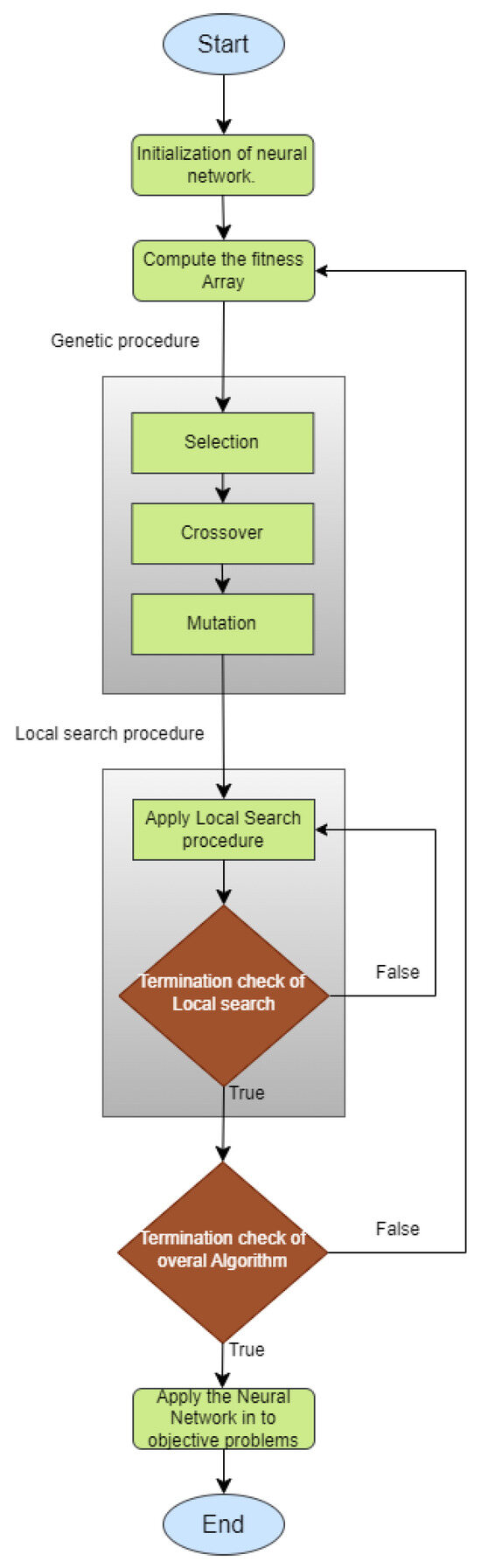
Figure 3. The flowchart of the proposed algorithm.

2.3. The Local Search Procedure

The local search procedure initiates from the vector $\overrightarrow{w}$ that is produced for any given chromosome g using the procedure described in Section 2.1. The procedure minimizes the error of Equation (1) with respect to vector $\overrightarrow{w}$. The minimization is performed within a value interval created around the initial point $\overrightarrow{w}$ keeping the network structure intact. The main steps of this procedure are given below:

1.

Set $d=\left(n+2\right)H$. This value denotes the total number of parameters for $N\left(\overrightarrow{x},\overrightarrow{w}\right)$.

2.

For $i=1,\dots ,d$do

(a)

Set $L_i=-F\times \left|w_i\right|$, the left bound of the minimization for the parameter i.

(b)

Set $R_i=F\times \left|w_i\right|$, the right bound of the minimization for the parameter i.

3.

EndFor

4.

Minimize the error function of Equation (1) for vector $\overrightarrow{w}$ inside the bounding box $\left[\overrightarrow{L},\overrightarrow{R}\right]$ using a local optimization procedure $\mathcal{L}\left(w\right)$. The BFGS method as modified by Powell [63] was incorporated in the conducted experiments.

As an example, consider a dataset with $n=2$ and the following constructed neural network:

$$N\left(\overrightarrow{x},\overrightarrow{w}\right)=2\sigma \left(1.5x_2-2.0\right)+2.5\sigma \left(-1.2x_1+3.7\right)$$

(5)

where the number of nodes is $H=2$. In this case, the vector $\overrightarrow{w}$ has the elements $\overrightarrow{w}=\left(2,0,1.5,-2,2.5,-1.2,0,3.7\right)$. If the parameter F has the value $F=2,$ then the bound vectors $\overrightarrow{L}$ and $\overrightarrow{R}$ are defined as

$$\begin{array}{ccc}\hfill \overrightarrow{L}& =& \left(-4,0,-3,-4,-5,-2.4,0,7.4\right)\hfill \\ \hfill \overrightarrow{R}& =& \left(4,0,3,4,5,2.4,0,7.4\right)\hfill \end{array}$$

Hence, the minimization method could not change the elements $w_2$ and $w_7$, and as a consequence, the architecture of the network remains intact.

3. Experimental Results

A series of classification and regression datasets was used in order to test the current work. Also, the suggested technique was compared against other established machine learning methods, and the results are reported. Furthermore, a series of experiments were executed to verify the sensitivity of the proposed technique with respect to the critical parameters presented earlier. The following URLs provide the used datasets:

1.

The UCI dataset repository, https://archive.ics.uci.edu/ml/index.php (accessed on 28 September 2024) [64].

2.

The Keel repository, https://sci2s.ugr.es/keel/datasets.php (accessed on 28 September 2024) [65].

3.

The Statlib URL http://lib.stat.cmu.edu/datasets/ (accessed on 28 September 2024).

3.1. The Used Classification Datasets

The descriptions of the used datasets are also provided:

1.

Appendictis, which is a dataset originated in [66].

2.

Australian dataset [67], which is related to bank transactions.

3.

Balance dataset [68], which has been used in a series of psychological experiments.

4.

Circular dataset, which contains artificially generated data.

5.

Cleveland dataset [69,70].

6.

Dermatology dataset [71], which is a dataset that contains measurements of dermatological deceases.

7.

Ecoli dataset, which is a dataset that contains measurements of proteins [72].

8.

Fert dataset, which is used to detect the relation between sperm concentration and demographic data.

9.

Haberman dataset, which is a medical dataset related to breast cancer.

10.

Hayes roth dataset [73].

11.

Heart dataset [74], which is a medical dataset used for the prediction of heart diseases.

12.

HeartAttack dataset, which is used for the detection of heart diseases.

13.

HouseVotes dataset [75].

14.

Liverdisorder dataset [76], which is a medical dataset.

15.

Ionosphere dataset, which is a climate dataset [77,78].

16.

Mammographic dataset [79], which is a dataset related to the breast cancer.

17.

Parkinsons dataset, which is used in the detection of Parkinson’s disease (PD) [80].

18.

Pima dataset [81].

19.

Popfailures dataset [82].

20.

Regions2 dataset, which is used in the detection of hepatitis C [83].

21.

Saheart dataset [84], which is a medical dataset used for the detection of heart diseases.

22.

Segment dataset [85], which is a dataset related to image processing.

23.

Spiral dataset, which is an artificial dataset.

24.

Student dataset [86], which contains data from experiments conducted in Portuguese schools.

25.

Transfusion dataset [87], which is a medical dataset.

26.

Wdbc dataset [88].

27.

Wine dataset, which is used for the detection of the quality of wines [89,90].

28.

Eeg datasets, which is a dataset that contains EEG experiments [91]. The following distinct cases were used from this dataset: Z_F_S, Z_O_N_F_S, ZO_NF_S and ZONF_S.

29.

Zoo dataset [92], which is used to classify animals.

The number of inputs and classes for every classification dataset is given in Table 1.

Table 1. Number of inputs and distinct classes for every classification dataset.

DATASET	INPUTS	CLASSES
APPENDICITIS	7	2
AUSTRALIAN	14	2
BALANCE	4	3
CIRCULAR	5	2
CLEVELAND	13	5
DERMATOLOGY	34	6
ECOLI	7	8
FERT	9	2
HABERMAN	3	2
HAYES ROTH	5	3
HEART	13	2
HEART ATTACK	13	2
HOUSEVOTES	16	2
LIVERDISORDER	6	2
IONOSPHERE	34	2
MAMMOGRAPHIC	5	2
PARKINSONS	22	2
PIMA	8	2
POPFAILURES	18	2
REGIONS2	18	5
SAHEART	9	2
SEGMENT	19	7
SPIRAL	2	2
STUDENT	5	4
TRANSFUSION	4	2
WDBC	30	2
WINE	13	3
Z_F_S	21	3
Z_O_N_F_S	21	5
ZO_NF_S	21	3
ZONF_S	21	2
ZOO	16	7

3.2. The Used Regression Datasets

The descriptions for these datasets are provided below:

1.

Abalone dataset [93].

2.

Airfoil dataset, which is a dataset derived from NASA [94].

3.

BK dataset [95], which contains data from various basketball games.

4.

BL dataset, which contains data from an electricity experiment.

5.

Baseball dataset, which is used to predict the average income of baseball players.

6.

Concrete dataset [96].

7.

Dee dataset, which contains measurements of the price of electricity.

8.

FY, which is used to measure the longevity of fruit flies.

9.

HO dataset, which appeared in the STALIB repository.

10.

Housing dataset, which originated in [97].

11.

Laser dataset, which contains data from physics experiments

12.

LW dataset, which contains measurements of low weight babies.

13.

MORTGAGE dataset, which is related to some economic measurements from the USA.

14.

MUNDIAL, which appeared in the STALIB repository.

15.

PL dataset, which is included in the STALIB repository.

16.

QUAKE dataset, which contains data about earthquakes.

17.

REALESTATE, which is included in the STALIB repository.

18.

SN dataset, which contains measurements from an experiment related to trellising and pruning.

19.

Treasury dataset, which deals with some factors of the USA economy.

20.

VE dataset, which is included in the STALIB repository.

21.

TZ dataset, which is included in the STALIB repository.

The number of inputs for each dataset is provided in Table 2.

Table 2. Number of inputs for every regression dataset.

DATASET	INPUTS
ABALONE	8
AIRFOIL	5
BASEBALL	16
BK	4
BL	7
CONCRETE	8
DEE	6
HO	13
HOUSING	13
FY	4
LASER	4
LW	9
MORTGAGE	15
MUNDIAL	3
PL	2
QUAKE	3
REALESTATE	5
SN	11
TREASURY	15
TZ	60
VE	7

3.3. Experimental Results

All the methods used here were coded in ANSI C++. The freely available optimization of Optimus, which can be downloaded from https://github.com/itsoulos/GlobalOptimus/ (accessed on 28 September 2024), was also utilized for the optimization process. Each experiment was conducted 30 times, and the average classification or regression value was measured. In each run, a different seed for the random number generator was used, and the drand48() function of the C programming language was incorporated. For the case of classification datasets, the displayed classification error for a model $M\left(x\right)$ and the test dataset T is calculated as

$$E_C\left(M\left(x\right)\right)=100\times {\displaystyle \frac{{\sum }_{i=1}^N\left(\mathrm{class}\left(M\left(x_i\right)\right)-y_i\right)}{N}}$$

(6)

The test set T is defined as $T=\left(x_i,y_i\right),i=1,\dots ,N$. For the case of regression problems, the regression error $E_R\left(M\left(x\right)\right)$ is defined as

$$E_R\left(M\left(x\right)\right)={\displaystyle \frac{{\sum }_{i=1}^N{\left(M\left(x_i\right)-y_i\right)}^2}{N}}$$

(7)

The method of ten-fold cross-validation was incorporated to validate the experimental results. The experiments were carried out on an AMD Ryzen 5950X with 128 GB of RAM, running the Debian Linux operating system. The values for the parameters of the algorithms are shown in Table 3. In all tables, the bold font is used to mark the machine learning method that achieved the lowest classification or regression error.

Table 3. The values of the parameters used in the experiments.

PARAMETER	MEANING	VALUE
$N_c$	Chromosomes	500
$N_g$	Generations	200
$p_s$	Crossover rate	0.10
$p_m$	Mutation rate	0.05
$N_T$	Number of chromosomes that selected randomly	20
$N_I$	Number of iterations before local search	10
F	Magnitude of changes from local search	4.0

Table 4 contains the experimental results for the classification datasets and Table 5 contains the experimental results for the regression datasets. The neural network used in the experimental results has one processing unit with $H=10$ processing nodes and the sigmoid function as an activation function. The following notation was used in these tables:

Table 4. Results from the application of machine learning models on the classification datasets. Numbers in cells represent average classification errors for the corresponding test set. The bold notation is used to mark the method with the lowest test error.

DATASET	BFGS	GENETIC	NNC	INNC
APPENDICITIS	18.00%	24.40%	13.70%	14.70%
AUSTRALIAN	38.13%	36.64%	14.51%	14.80%
BALANCE	8.64%	8.36%	22.11%	8.66%
CIRCULAR	6.08%	5.13%	13.64%	5.32%
CLEVELAND	77.55%	57.21%	50.10%	47.93%
DERMATOLOGY	52.92%	16.60%	25.06%	20.89%
ECOLI	69.52%	54.67%	47.82%	48.21%
FERT	23.20%	28.50%	19.00%	20.50%
HABERMAN	29.34%	28.66%	28.03%	26.70%
HAYES-ROTH	37.33%	56.18%	35.93%	31.77%
HEART	39.44%	26.41%	15.78%	14.74%
HEARTATTACK	46.67%	29.03%	19.33%	20.43%
HOUSEVOTES	7.13%	7.00%	3.65%	3.26%
IONOSPHERE	15.29%	15.14%	11.12%	11.92%
LIVERDISORDER	42.59%	37.09%	33.71%	31.77%
MAMMOGRAPHIC	17.24%	19.88%	17.78%	15.81%
PARKINSONS	27.58%	16.58%	12.21%	12.53%
PIMA	35.59%	34.21%	27.99%	24.00%
POPFAILURES	5.24%	4.17%	6.74%	6.44%
REGIONS2	36.28%	33.53%	25.52%	23.18%
SAHEART	37.48%	34.85%	30.52%	28.09%
SEGMENT	68.97%	46.30%	54.99%	43.12%
SPIRAL	47.99%	47.67%	48.39%	43.99%
STUDENT	7.14%	5.61%	5.78%	4.55%
TRANSFUSION	25.80%	25.84%	25.34%	23.43%
WDBC	29.91%	7.87%	6.95%	4.41%
WINE	59.71%	22.88%	14.35%	9.77%
Z_F_S	39.37%	24.60%	14.17%	8.53%
Z_O_N_F_S	65.67%	64.81%	49.18%	38.58%
ZO_NF_S	43.04%	21.54%	14.14%	6.84%
ZONF_S	15.62%	4.36%	3.14%	2.52%
ZOO	10.70%	9.50%	9.20%	7.20%
AVERAGE	33.91%	26.73%	22.50%	19.52%

Table 5. Results from the conducted experiments on the regression datasets. Numbers in cells denote average regression errors as calculated on the corresponding test sets. The bold notation is used to mark the method with the lowest test error.

DATASET	BFGS	GENETIC	NNC	INNC
ABALONE	5.69	7.17	5.05	4.33
AIRFOIL	0.003	0.003	0.003	0.002
BASEBALL	119.63	64.60	59.85	48.42
BK	0.36	0.26	2.32	0.07
BL	1.09	2.23	0.021	0.002
CONCRETE	0.066	0.01	0.008	0.005
DEE	2.36	1.01	0.26	0.23
HO	0.62	0.37	0.017	0.01
HOUSING	97.38	43.26	26.35	16.01
FY	0.19	0.65	0.058	0.042
LASER	0.015	0.59	0.024	0.005
LW	2.98	0.54	0.011	0.012
MORTGAGE	8.23	0.40	0.30	0.026
MUNDIAL	6.48	1.22	4.47	0.034
PL	0.29	0.28	0.045	0.022
QUAKE	0.42	0.12	0.045	0.04
REALESTATE	128.94	81.19	76.78	70.99
SN	3.89	0.40	0.026	0.023
TREASURY	9.91	2.93	0.47	0.066
TZ	3.27	5.38	5.04	0.03
VE	1.92	2.43	6.61	0.025
AVERAGE	18.75	10.24	8.94	6.69

1.

The column BFGS represents the results obtained by the application of the BFGS method to train a neural network with $H=10$ processing nodes.

2.

The column GENETIC represents the results produced by the training of a neural network with $H=10$ processing nodes using a genetic algorithm. The parameters of this algorithm are mentioned in Table 3.

3.

The column NNC represents the results obtained by the neural construction technique.

4.

The column INNC represents the results obtained by the proposed method.

5.

The last row AVERAGE contains the average classification or regression error, as measured on all datasets.

The methods BFGS and GENETIC train the neural network $N\left(\overrightarrow{x},\overrightarrow{w}\right)$ by obtaining the global minimum of the error function defined in Equation (1).

The original technique of constructing artificial neural networks has significantly lower classification or regression errors than the other two techniques, and the proposed method managed to improve the performance of this technique in the majority of the datasets. The percentage improvement in error is even greater in regression problems. In some cases, the improvement exceeds 50% in the test error. This effect is evident in the box plots for classification and regression errors outlined in Figure 4 and Figure 5, respectively.

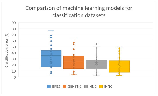
Figure 4. Box plot for the comparison between the machine learning methods applied on the classification datasets.

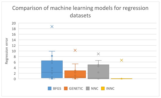
Figure 5. Box plot for the comparison between the machine learning methods applied on the regression datasets.

Furthermore, the same reduction in test error is validated from the statistical tests performed for classification and regression problems. These tests are depicted in Figure 6 and Figure 7.

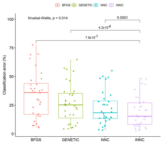
Figure 6. Statistical test for all machine learning models that was applied on the classification datasets.

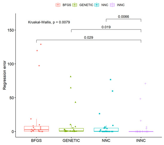
Figure 7. Statistical test for all machine learning models that was applied on the regression datasets.

3.3.1. Experiments with the Parameter $N_I$

To verify the robustness of the proposed technique as well as its sensitivity to parameter changes, a new experiment was carried out in which the critical $N_I$ parameter was varied from 5 to 20. This parameter determines the number of generations intervening before the local optimization method is executed on randomly selected chromosomes. The results from this experiment for the classification datasets are depicted in Table 6, and the results for the regression datasets are depicted in Table 7.

Table 6. Experimental results using a variety of values for the parameter $N_I$ of the current work with application on the classification datasets. The bold notation marks the method with the lowest test error.

DATASET	INNC $\left({\mathit{N}}_{\mathit{I}}=5\right)$	INNC $\left({\mathit{N}}_{\mathit{I}}=10\right)$	INNC $\left({\mathit{N}}_{\mathit{I}}=20\right)$
APPENDICITIS	14.50%	14.70%	14.20%
AUSTRALIAN	14.48%	14.80%	14.58%
BALANCE	7.63%	8.66%	11.71%
CIRCULAR	5.25%	5.32%	5.87%
CLEVELAND	48.41%	47.93%	49.66%
DERMATOLOGY	19.66%	20.89%	23.11%
ECOLI	47.39%	48.21%	48.09%
FERT	20.80%	20.50%	20.90%
HABERMAN	26.87%	26.70%	27.27%
HAYES-ROTH	31.69%	31.77%	35.92%
HEART	14.85%	14.74%	15.56%
HEARTATTACK	20.10%	20.43%	20.07%
HOUSEVOTES	3.87%	3.26%	3.78%
IONOSPHERE	11.51%	11.92%	11.09%
LIVERDISORDER	31.35%	31.77%	31.85%
MAMMOGRAPHIC	16.25%	15.81%	16.06%
PARKINSONS	13.16%	12.53%	12.58%
PIMA	23.95%	24.00%	24.67%
POPFAILURES	6.06%	6.44%	6.48%
REGIONS2	23.36%	23.18%	24.21%
SAHEART	27.68%	28.09%	29.41%
SEGMENT	43.79%	43.12%	46.91%
SPIRAL	43.63%	43.99%	45.15%
STUDENT	3.65%	4.55%	3.88%
TRANSFUSION	22.62%	23.43%	23.89%
WDBC	4.41%	4.41%	5.46%
WINE	10.18%	9.77%	12.00%
Z_F_S	7.70%	8.53%	9.63%
Z_O_N_F_S	36.64%	38.58%	41.08%
ZO_NF_S	6.84%	6.84%	6.90%
ZONF_S	2.24%	2.52%	2.66%
ZOO	6.30%	7.20%	7.70%
AVERAGE	19.28%	19.52%	20.39%

Table 7. Experimental results with a variety of values for the parameter $N_I$. The current work was applied on the regression datasets. The bold notation marks the method with the lowest test error.

DATASET	INNC $\left({\mathit{N}}_{\mathit{I}}=5\right)$	INNC $\left({\mathit{N}}_{\mathit{I}}=10\right)$	INNC $\left({\mathit{N}}_{\mathit{I}}=20\right)$
ABALONE	4.38	4.33	4.45
AIRFOIL	0.002	0.002	0.002
BASEBALL	47.50	48.42	49.99
BK	0.64	0.07	1.86
BL	0.014	0.002	0.003
CONCRETE	0.005	0.005	0.005
DEE	0.22	0.23	0.23
HO	0.01	0.01	0.011
HOUSING	21.09	16.01	16.96
FY	0.046	0.042	0.19
LASER	0.004	0.005	0.005
LW	0.011	0.012	0.011
MORTGAGE	0.02	0.026	0.03
MUNDIAL	0.031	0.034	0.029
PL	0.022	0.022	0.022
QUAKE	0.045	0.04	0.037
REALESTATE	68.85	70.99	70.59
SN	0.023	0.023	0.024
TREASURY	0.063	0.066	0.073
TZ	0.029	0.03	0.031
VE	0.028	0.025	0.116
AVERAGE	6.81	6.69	6.89

The method appears to have similar results for each variation of the critical $N_I$ parameter. In some cases, the error is smaller for low values of this parameter but not to a great extent. This effect is also evident in the box plot presented for the classification datasets in Figure 8 as well as in the statistical comparison of Figure 9.

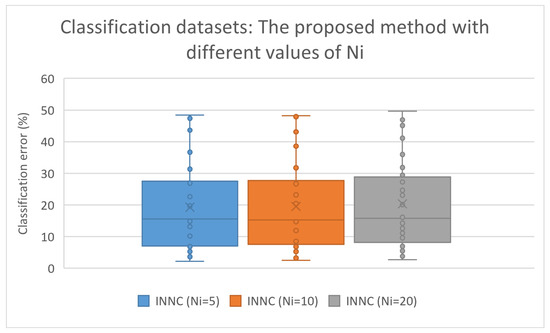
Figure 8. Box plot for the experiments with the parameter $N_I$ and the current work. The method was applied on the classification datasets.

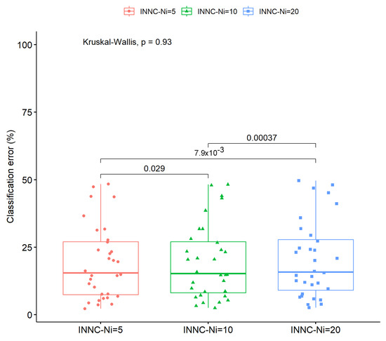
Figure 9. Statistical comparison of the experiment with the current work and a variety of values for parameter $N_I$. The method was applied on the classification datasets.

In addition, the average execution time of the methods was recorded for the various values of the parameter $N_I$, and the results are shown in Figure 10 and Figure 11 for classification and regression problems, respectively.

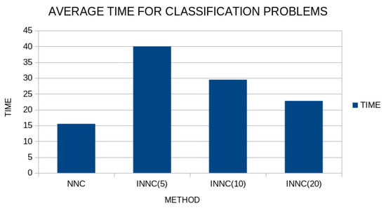
Figure 10. Average execution time for the original method and the modified one. The time was recorded for different values of the parameter $N_I$ and for the classification datasets.

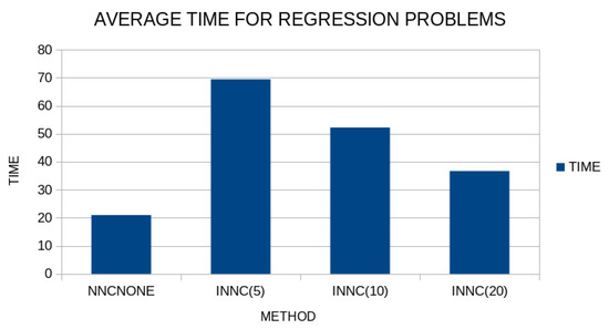
Figure 11. Average execution time for the original method and the modified one. The time was measured for different values of the parameter $N_I$. The execution times were recorded for the regression problems.

As expected, the method requires more computational time than the original one, and in fact, the smaller the value of the $N_I$ parameter the more time has to be spent since more local optimizations have to be performed. Of course, this additional computing time can be significantly reduced by using parallel computing techniques.

3.3.2. Experiments with the Parameter F

Another important parameter for the proposed method is parameter F. This parameter identifies the range of changes that the local optimization method can cause on randomly selected chromosomes. In this experiment, the parameter F changed from 1.5 to 8.0, and the results for the classification datasets are depicted in Table 8, while the experimental results for the regression datasets are presented in Table 9.

Table 8. Experimental results with a variety of values for the parameter F with application on the classification datasets. The bold notation marks the method with the lowest test error.

DATASET	INNC $\left(\mathit{F}=1.5\right)$	INNC $\left(\mathit{F}=2.0\right)$	INNC $\left(\mathit{F}=4.0\right)$	INNC $\left(\mathit{F}=8.0\right)$
APPENDICITIS	14.80%	14.20%	14.70%	15.00%
AUSTRALIAN	14.58%	14.56%	14.80%	14.54%
BALANCE	8.52%	8.68%	8.66%	9.35%
CIRCULAR	5.92%	5.46%	5.32%	5.43%
CLEVELAND	48.35%	47.38%	47.93%	49.62%
DERMATOLOGY	19.80%	20.09%	20.89%	21.66%
ECOLI	47.76%	48.30%	48.21%	48.42%
FERT	21.20%	21.20%	20.50%	20.90%
HABERMAN	26.43%	25.93%	26.70%	26.70%
HAYES-ROTH	32.15%	31.31%	31.77%	35.69%
HEART	14.81%	15.41%	14.74%	15.41%
HEARTATTACK	21.20%	19.90%	20.43%	20.40%
HOUSEVOTES	3.35%	3.65%	3.26%	3.65%
IONOSPHERE	11.31%	10.40%	11.92%	11.23%
LIVERDISORDER	32.09%	31.21%	31.77%	33.18%
MAMMOGRAPHIC	16.15%	16.05%	15.81%	16.07%
PARKINSONS	12.63%	12.47%	12.53%	13.05%
PIMA	23.58%	23.80%	24.00%	23.79%
POPFAILURES	5.85%	6.29%	6.44%	6.04%
REGIONS2	24.08%	23.48%	23.18%	25.25%
SAHEART	28.41%	28.83%	28.09%	28.30%
SEGMENT	45.12%	43.37%	43.12%	43.93%
SPIRAL	43.40%	43.72%	43.99%	44.61%
STUDENT	4.25%	4.15%	4.55%	4.52%
TRANSFUSION	23.09%	22.93%	23.43%	23.05%
WDBC	5.27%	5.30%	4.41%	4.84%
WINE	10.53%	10.24%	9.77%	11.59%
Z_F_S	9.20%	7.57%	8.53%	8.63%
Z_O_N_F_S	40.60%	38.70%	38.58%	39.78%
ZO_NF_S	6.90%	7.68%	6.84%	6.56%
ZONF_S	2.64%	2.72%	2.52%	2.88%
ZOO	8.60%	7.40%	7.20%	8.90%
AVERAGE	19.77%	19.45%	19.52%	20.09%

Table 9. Experimental results using a variety of values for the parameter F with application on the the regression datasets. The bold notation marks the method with the lowest test error.

DATASET	INNC $\left(\mathit{F}=1.5\right)$	INNC $\left(\mathit{F}=2.0\right)$	INNC $\left(\mathit{F}=4.0\right)$	INNC $\left(\mathit{F}=8.0\right)$
ABALONE	4.49	4.43	4.33	4.66
AIRFOIL	0.002	0.002	0.002	0.002
BASEBALL	48.31	50.38	48.42	48.52
BK	0.06	0.21	0.07	0.02
BL	0.003	0.004	0.002	0.003
CONCRETE	0.005	0.005	0.005	0.005
DEE	0.23	0.23	0.23	0.23
HO	0.01	0.01	0.01	0.01
HOUSING	16.91	16.34	16.01	16.96
FY	0.042	0.043	0.042	0.043
LASER	0.005	0.005	0.005	0.004
LW	0.011	0.012	0.012	0.012
MORTGAGE	0.027	0.025	0.026	0.024
MUNDIAL	0.035	0.033	0.034	0.23
PL	0.022	0.022	0.022	0.022
QUAKE	0.036	0.037	0.04	0.036
REALESTATE	72.40	71.16	70.99	70.76
SN	0.024	0.024	0.023	0.024
TREASURY	0.07	0.068	0.066	0.068
TZ	0.029	0.031	0.03	0.031
VE	0.032	0.03	0.025	0.028
AVERAGE	6.80	6.81	6.69	6.75

Once again, there are no significant differences in the performance of the proposed technique as the critical factor F varies. In the case of the classification data, however, there is a small increase in the classification error as this factor increases, which may be due to the fact that as we move away from the solution created by the method of creating neural networks, the performance of the method decreases. Also, the box plot for the classification datasets is depicted in Figure 12.

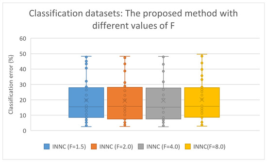
Figure 12. Box plot for the experiments using the current work and different values of the parameter F. The experiments were conducted on the classification datasets.

3.3.3. Experiments with the Used Local Search Optimizer

An important issue of the proposed method is the selection of the local search optimizer, that will be applied periodically to chromosomes selected randomly. In the current work, a modified version of the BFGS method [63] was chosen, since it can satisfactorily handle the constraints placed on the network parameters for the optimization. However, an additional experiment was executed using different local optimization techniques. The results for the classification datasets are presented in Table 10, and the results for the regression datasets are shown in Table 11. The following notation is used in the experimental tables:

Table 10. Experimental results with different local optimization techniques in the proposed method with application on the classification datasets. The bold notation marks the method with the lowest test error.

DATASET	ADAM	LBFGS	BFGS
APPENDICITIS	14.60%	14.60%	14.70%
AUSTRALIAN	14.78%	15.29%	14.80%
BALANCE	16.89%	11.47%	8.66%
CIRCULAR	10.79%	8.15%	5.32%
CLEVELAND	49.10%	48.45%	47.93%
DERMATOLOGY	22.32%	23.03%	20.89%
ECOLI	48.15%	49.48%	48.21%
FERT	18.10%	20.10%	20.50%
HABERMAN	26.27%	26.63%	26.70%
HAYES-ROTH	36.23%	36.31%	31.77%
HEART	15.71%	15.00%	14.74%
HEARTATTACK	21.33%	20.07%	20.43%
HOUSEVOTES	3.39%	3.39%	3.26%
IONOSPHERE	10.88%	11.29%	11.92%
LIVERDISORDER	31.80%	33.18%	31.77%
MAMMOGRAPHIC	16.71%	16.30%	15.81%
PARKINSONS	12.10%	12.32%	12.53%
PIMA	25.49%	24.97%	24.00%
POPFAILURES	6.20%	6.31%	6.44%
REGIONS2	24.20%	24.06%	23.18%
SAHEART	28.87%	28.96%	28.09%
SEGMENT	50.16%	46.63%	43.12%
SPIRAL	46.33%	45.24%	43.99%
STUDENT	4.05%	3.98%	4.55%
TRANSFUSION	24.74%	24.56%	23.43%
WDBC	6.30%	5.66%	4.41%
WINE	11.47%	10.06%	9.77%
Z_F_S	12.33%	10.92%	8.53%
Z_O_N_F_S	41.40%	45.77%	38.58%
ZO_NF_S	11.26%	9.83%	6.84%
ZONF_S	2.64%	2.35%	2.52%
ZOO	8.50%	8.70%	7.20%
AVERAGE	21.03%	20.72%	19.52%

Table 11. Experimental results with local optimization techniques in the current work with application on the regression datasets. The bold notation marks the method with the lowest test error.

DATASET	ADAM	LBFGS	BFGS
ABALONE	4.73	4.49	4.33
AIRFOIL	0.003	0.003	0.002
BASEBALL	53.98	51.88	48.42
BK	0.05	0.08	0.07
BL	0.013	0.007	0.002
CONCRETE	0.006	0.006	0.005
DEE	0.24	0.23	0.23
HO	0.012	0.012	0.01
HOUSING	20.20	20.49	16.01
FY	0.042	0.042	0.042
LASER	0.012	0.005	0.005
LW	0.011	0.011	0.012
MORTGAGE	0.068	0.084	0.026
MUNDIAL	0.033	0.029	0.034
PL	0.031	0.023	0.022
QUAKE	0.036	0.037	0.04
REALESTATE	74.66	74.49	70.99
SN	0.025	0.024	0.023
TREASURY	0.114	0.084	0.066
TZ	0.03	0.08	0.03
VE	0.024	0.132	0.025
AVERAGE	7.35	7.25	6.69

1.

The column ADAM denotes the incorporation of the ADAM local optimization method [18] in the current technique.

2.

The column LBFGS denotes the incorporation of the Limited Memory BFGS (L-BFGS) method [98] as the local search procedure.

3.

The column BFGS represents the incorporation of the BFGS method, modified by Powell [63], as the local search procedure.

The BFGS method achieved lower values for the test error in the majority of cases, and this is also evident in Figure 13, where a box plot is depicted for the classification datasets.

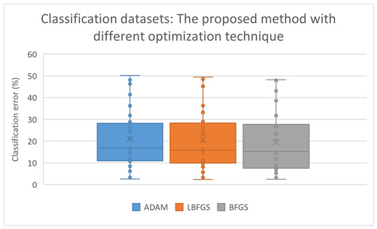
Figure 13. Box plot for the experiment with the proposed method and different local optimization methods. The current work was executed on the classification datasets.

4. Conclusions

An extension of the artificial neural network construction technique was presented in the present work, in which the continuous application of a local optimization method to chromosomes that were selected randomly was introduced. The local optimization method was applied in such a way as not to alter the architecture of the neural network constructed by grammatical evolution. The proposed modified method was applied on a series of benchmark datasets found in the relevant literature and, judging from the experimental results, it reduced significantly the test error of the original method in most datasets.

Moreover, to establish the stability of the proposed technique, additional experiments were carried out in which a number of critical parameters were varied over a range of values. After the completion of these experiments, it became clear that there is no significant difference in the effectiveness of the proposed method even if these critical parameters change significantly from execution to execution. The only case where a significant difference in the effectiveness of the proposed technique was found was when different local optimization techniques were used, where the BFGS variant appeared to achieve the best results in the majority of cases.

Nevertheless, one major drawback of the current work is the additional execution time required from the execution of the local search optimization techniques. Since the grammatical evolution procedure is a modified genetic algorithm, the generated artificial neural networks are independent of themselves, and parallel programming techniques may be used in order to improve the speed of the method, such as the usage of MPI [99] or the OpenMP library [100].

References

- Abiodun, O.I.; Jantan, A.; Omolara, A.E.; Dada, K.V.; Mohamed, N.A.; Arshad, H. State-of-the-art in artificial neural network applications: A survey. Heliyon 2018, 4, e00938. [Google Scholar] [CrossRef]
- Suryadevara, S.; Yanamala, A.K.Y. A Comprehensive Overview of Artificial Neural Networks: Evolution, Architectures, and Applications. Rev. Intel. Artif. Med. 2021, 12, 51–76. [Google Scholar]
- Baldi, P.; Cranmer, K.; Faucett, T.; Sadowski, P.; Whiteson, D. Parameterized neural networks for high-energy physics. Eur. Phys. J. C 2016, 76, 1–7. [Google Scholar] [CrossRef]
- Carleo, G.; Troyer, M. Solving the quantum many-body problem with artificial neural networks. Science 2017, 355, 602–606. [Google Scholar] [CrossRef]
- Khoo, Y.; Lu, J.; Ying, L. Solving parametric PDE problems with artificial neural networks. Eur. J. Appl. Math. 2021, 32, 421–435. [Google Scholar] [CrossRef]
- Kumar Yadav, A.; Chandel, S.S. Solar radiation prediction using Artificial Neural Network techniques: A review. Renew. Sustain. Energy Rev. 2014, 33, 772–781. [Google Scholar] [CrossRef]
- Escamilla-García, A.; Soto-Zarazúa, G.M.; Toledano-Ayala, M.; Rivas-Araiza, E.; Gastélum-Barrios, A. Applications of Artificial Neural Networks in Greenhouse Technology and Overview for Smart Agriculture Development. Appl. Sci. 2020, 10, 3835. [Google Scholar] [CrossRef]
- Shen, L.; Wu, J.; Yang, W. Multiscale Quantum Mechanics/Molecular Mechanics Simulations with Neural Networks. J. Chem. Theory Comput. 2016, 12, 4934–4946. [Google Scholar] [CrossRef]
- Wei, J.N.; Duvenaud, D.; Aspuru-Guzik, A. Neural Networks for the Prediction of Organic Chemistry Reactions. ACS Cent. Sci. 2016, 2, 725–732. [Google Scholar] [CrossRef]
- Khosravi, A.; Koury, R.N.N.; Machado, L.; Pabon, J.J.G. Prediction of wind speed and wind direction using artificial neural network, support vector regression and adaptive neuro-fuzzy inference system. Sustain. Energy Technol. Assess. 2018, 25, 146–160. [Google Scholar] [CrossRef]
- Falat, L.; Pancikova, L. Quantitative Modelling in Economics with Advanced Artificial Neural Networks. Procedia Econ. Financ. 2015, 34, 194–201. [Google Scholar] [CrossRef]
- Namazi, M.; Shokrolahi, A.; Sadeghzadeh Maharluie, M. Detecting and ranking cash flow risk factors via artificial neural networks technique. J. Bus. Res. 2016, 69, 1801–1806. [Google Scholar] [CrossRef]
- Baskin, I.I.; Winkler, D.; Tetko, I.V. A renaissance of neural networks in drug discovery. Expert Opin. Drug Discov. 2016, 11, 785–795. [Google Scholar] [CrossRef]
- Bartzatt, R. Prediction of Novel Anti-Ebola Virus Compounds Utilizing Artificial Neural Network (ANN). Chem. Fac. Publ. 2018, 49, 16–34. [Google Scholar]
- Vora, K.; Yagnik, S. A survey on backpropagation algorithms for feedforward neural networks. Int. J. Eng. Dev. Res. 2014, 1, 193–197. [Google Scholar]
- Pajchrowski, T.; Zawirski, K.; Nowopolski, K. Neural speed controller trained online by means of modified RPROP algorithm. IEEE Trans. Ind. Inform. 2014, 11, 560–568. [Google Scholar] [CrossRef]
- Hermanto, R.P.S.; Nugroho, A. Waiting-time estimation in bank customer queues using RPROP neural networks. Procedia Comput. Sci. 2018, 135, 35–42. [Google Scholar] [CrossRef]
- Kingma, D.P.; Ba, J.L. ADAM: A method for stochastic optimization. In Proceedings of the 3rd International Conference on Learning Representations (ICLR 2015), San Diego, CA, USA, 7–9 May 2015; pp. 1–15. [Google Scholar]
- Kuo, C.L.; Kuruoglu, E.E.; Chan, W.K.V. Neural Network Structure Optimization by Simulated Annealing. Entropy 2022, 24, 348. [Google Scholar] [CrossRef]
- Reynolds, J.; Rezgui, Y.; Kwan, A.; Piriou, S. A zone-level, building energy optimisation combining an artificial neural network, a genetic algorithm, and model predictive control. Energy 2018, 151, 729–739. [Google Scholar] [CrossRef]
- Das, G.; Pattnaik, P.K.; Padhy, S.K. Artificial neural network trained by particle swarm optimization for non-linear channel equalization. Expert Syst. Appl. 2014, 41, 3491–3496. [Google Scholar] [CrossRef]
- Wang, L.; Zeng, Y.; Chen, T. Back propagation neural network with adaptive differential evolution algorithm for time series forecasting. Expert Syst. Appl. 2015, 42, 855–863. [Google Scholar] [CrossRef]
- Salama, K.M.; Abdelbar, A.M. Learning neural network structures with ant colony algorithms. Swarm Intell. 2015, 9, 229–265. [Google Scholar] [CrossRef]
- Mirjalili, S. How effective is the Grey Wolf optimizer in training multi-layer perceptrons. Appl. Intell. 2015, 43, 150–161. [Google Scholar] [CrossRef]
- Aljarah, I.; Faris, H.; Mirjalili, S. Optimizing connection weights in neural networks using the whale optimization algorithm. Soft Comput. 2018, 22, 1–15. [Google Scholar] [CrossRef]
- Zhang, M.; Hibi, K.; Inoue, J. GPU-accelerated artificial neural network potential for molecular dynamics simulation. Comput. Phys. Commun. 2023, 285, 108655. [Google Scholar] [CrossRef]
- Varnava, T.M.; Meade, A.J. An initialization method for feedforward artificial neural networks using polynomial bases. Adv. Adapt. Data Anal. 2011, 3, 385–400. [Google Scholar] [CrossRef]
- Ivanova, I.; Kubat, M. Initialization of neural networks by means of decision trees. Knowl.-Based Syst. 1995, 8, 333–344. [Google Scholar] [CrossRef]
- Sodhi, S.S.; Chandra, P. Interval based Weight Initialization Method for Sigmoidal Feedforward Artificial Neural Networks. AASRI Procedia 2014, 6, 19–25. [Google Scholar] [CrossRef]
- Chumachenko, K.; Iosifidis, A.; Gabbouj, M. Feedforward neural networks initialization based on discriminant learning. Neural Netw. 2022, 146, 220–229. [Google Scholar] [CrossRef]
- Chen, Q.; Hao, W.; He, J. A weight initialization based on the linear product structure for neural networks. Appl. Math. Comput. 2022, 415, 126722. [Google Scholar] [CrossRef]
- Arifovic, J.; Gençay, R. Using genetic algorithms to select architecture of a feedforward artificial neural network. Phys. A Stat. Mech. Its Appl. 2001, 289, 574–594. [Google Scholar] [CrossRef]
- Benardos, P.G.; Vosniakos, G.C. Optimizing feedforward artificial neural network architecture. Eng. Appl. Artif. Intell. 2007, 20, 365–382. [Google Scholar] [CrossRef]
- Garro, B.A.; Vázquez, R.A. Designing Artificial Neural Networks Using Particle Swarm Optimization Algorithms. Comput. Intell. Neurosci. 2015, 2015, 369298. [Google Scholar] [CrossRef]
- Baker, B.; Gupta, O.; Naik, N.; Raskar, R. Designing neural network architectures using reinforcement learning. arXiv 2016, arXiv:1611.02167. [Google Scholar]
- Islam, M.M.; Sattar, M.A.; Amin, M.F.; Yao, X.; Murase, K. A New Adaptive Merging and Growing Algorithm for Designing Artificial Neural Networks. IEEE Trans. Syst. Man Cybern. Part B (Cybern.) 2009, 39, 705–722. [Google Scholar] [CrossRef] [PubMed]
- O’Neill, M.; Ryan, C. Grammatical evolution. IEEE Trans. Evol. Comput. 2001, 5, 349–358. [Google Scholar] [CrossRef]
- Tsoulos, I.G.; Gavrilis, D.; Glavas, E. Neural network construction and training using grammatical evolution. Neurocomputing 2008, 72, 269–277. [Google Scholar] [CrossRef]
- Papamokos, G.V.; Tsoulos, I.G.; Demetropoulos, I.N.; Glavas, E. Location of amide I mode of vibration in computed data utilizing constructed neural networks. Expert Syst. Appl. 2009, 36, 12210–12213. [Google Scholar] [CrossRef]
- Tsoulos, I.G.; Gavrilis, D.; Glavas, E. Solving differential equations with constructed neural networks. Neurocomputing 2009, 72, 2385–2391. [Google Scholar] [CrossRef]
- Tsoulos, I.G.; Mitsi, G.; Stavrakoudis, A.; Papapetropoulos, S. Application of Machine Learning in a Parkinson’s Disease Digital Biomarker Dataset Using Neural Network Construction (NNC) Methodology Discriminates Patient Motor Status. Front. ICT 2019, 6, 10. [Google Scholar] [CrossRef]
- Christou, V.; Tsoulos, I.G.; Loupas, V.; Tzallas, A.T.; Gogos, C.; Karvelis, P.S.; Antoniadis, N.; Glavas, E.; Giannakeas, N. Performance and early drop prediction for higher education students using machine learning. Expert Syst. Appl. 2023, 225, 120079. [Google Scholar] [CrossRef]
- Toki, E.I.; Pange, J.; Tatsis, G.; Plachouras, K.; Tsoulos, I.G. Utilizing Constructed Neural Networks for Autism Screening. Appl. Sci. 2024, 14, 3053. [Google Scholar] [CrossRef]
- Tsoulos, I.G.; Tzallas, A.; Tsalikakis, D. NNC: A tool based on Grammatical Evolution for data classification and differential equation solving. SoftwareX 2019, 10, 100297. [Google Scholar] [CrossRef]
- Backus, J.W. The Syntax and Semantics of the Proposed International Algebraic Language of the Zurich ACM-GAMM Conference. In Proceedings of the International Conference on Information Processing, UNESCO, Paris, France, 15–20 June 1959; pp. 125–132. [Google Scholar]
- Ryan, C.; Collins, J.; O’Neill, M. Grammatical evolution: Evolving programs for an arbitrary language. In Genetic Programming. EuroGP 1998; Banzhaf, W., Poli, R., Schoenauer, M., Fogarty, T.C., Eds.; Lecture Notes in Computer Science; Springer: Berlin/Heidelberg, Germany, 1998; Volume 1391. [Google Scholar]
- O’Neill, M.; Ryan, M.C. Evolving Multi-line Compilable C Programs. In Genetic Programming. EuroGP 1999; Poli, R., Nordin, P., Langdon, W.B., Fogarty, T.C., Eds.; Lecture Notes in Computer Science; Springer: Berlin/Heidelberg, Germany, 1999; Volume 1598. [Google Scholar]
- Ryan, C.; O’Neill, M.; Collins, J.J. Grammatical Evolution: Solving Trigonometric Identities. In Proceedings of the Mendel 1998: 4th International Mendel Conference on Genetic Algorithms, Optimisation Problems, Fuzzy Logic, Neural Networks, Rough Sets, Brno, Czech Republic, 1–2 November 1998. [Google Scholar]
- Puente, A.O.; Alfonso, R.S.; Moreno, M.A. Automatic composition of music by means of grammatical evolution. In APL ’02: Proceedings of the 2002 Conference on APL: Array Processing Languages: Lore, Problems, and Applications Madrid, Spain, 22–25 July 2002; Association for Computing Machinery: New York, NY, USA, 2002; pp. 148–155. [Google Scholar]
- Dempsey, I.; Neill, M.O.; Brabazon, A. Constant creation in grammatical evolution. Int. J. Innov. Comput. Appl. 2007, 1, 23–38. [Google Scholar] [CrossRef]
- Galván-López, E.; Swafford, J.M.; O’Neill, M.; Brabazon, A. Evolving a Ms. PacMan Controller Using Grammatical Evolution. In Applications of Evolutionary Computation. EvoApplications 2010; Lecture Notes in Computer Science; Springer: Berlin/Heidelberg, Germany, 2010; Volume 6024. [Google Scholar]
- Shaker, N.; Nicolau, M.; Yannakakis, G.N.; Togelius, J.; O’Neill, M. Evolving levels for Super Mario Bros using grammatical evolution. In Proceedings of the 2012 IEEE Conference on Computational Intelligence and Games (CIG), Granada, Spain, 11–14 September 2012; pp. 304–331. [Google Scholar]
- Martínez-Rodríguez, D.; Colmenar, J.M.; Hidalgo, J.I.; Micó, R.J.V.; Salcedo-Sanz, S. Particle swarm grammatical evolution for energy demand estimation. Energy Sci. Eng. 2020, 8, 1068–1079. [Google Scholar] [CrossRef]
- Sabar, N.R.; Ayob, M.; Kendall, G.; Qu, R. Grammatical Evolution Hyper-Heuristic for Combinatorial Optimization Problems. IEEE Trans. Evol. Comput. 2013, 17, 840–861. [Google Scholar] [CrossRef]
- Ryan, C.; Kshirsagar, M.; Vaidya, G.; Cunningham, A.; Sivaraman, R. Design of a cryptographically secure pseudo random number generator with grammatical evolution. Sci. Rep. 2022, 12, 8602. [Google Scholar] [CrossRef]
- Pereira, P.J.; Cortez, P.; Mendes, R. Multi-objective Grammatical Evolution of Decision Trees for Mobile Marketing user conversion prediction. Expert Syst. Appl. 2021, 168, 114287. [Google Scholar] [CrossRef]
- Castejón, F.; Carmona, E.J. Automatic design of analog electronic circuits using grammatical evolution. Appl. Soft Comput. 2018, 62, 1003–1018. [Google Scholar] [CrossRef]
- Araujo, L.; Martinez-Romo, J.; Duque, A. Discovering taxonomies in Wikipedia by means of grammatical evolution. Soft Comput. 2018, 22, 2907–2919. [Google Scholar] [CrossRef]
- Martín, C.; Quintana, D.; Isasi, P. Grammatical Evolution-based ensembles for algorithmic trading. Appl. Soft Comput. 2019, 84, 105713. [Google Scholar] [CrossRef]
- Moore, J.H.; Sipper, M. Grammatical Evolution Strategies for Bioinformatics and Systems Genomics. In Handbook of Grammatical Evolution; Ryan, C., O’Neill, M., Collins, J., Eds.; Springer: Cham, Switzerland, 2018. [Google Scholar] [CrossRef]
- Peabody, C.; Seitzer, J. GEF: A self-programming robot using grammatical evolution. In Proceedings of the AAAI Conference on Artificial Intelligence, Austin, TX, USA, 25–30 January 2015; Volume 29. [Google Scholar]
- Hornik, K.; Stinchcombe, M.; White, H. Multilayer feedforward networks are universal approximators. Neural Netw. 1989, 2, 359–366. [Google Scholar] [CrossRef]
- Powell, M.J.D. A Tolerant Algorithm for Linearly Constrained Optimization Calculations. Math. Program. 1989, 45, 547–566. [Google Scholar] [CrossRef]
- Kelly, M.; Longjohn, R.; Nottingham, K. The UCI Machine Learning Repository. 2023. Available online: https://archive.ics.uci.edu (accessed on 18 February 2024).
- Alcalá-Fdez, J.; Fernandez, A.; Luengo, J.; Derrac, J.; García, S.; Sánchez, L.; Herrera, F. KEEL Data-Mining Software Tool: Data Set Repository, Integration of Algorithms and Experimental Analysis Framework. J. Mult.-Valued Log. Soft Comput. 2011, 17, 255–287. [Google Scholar]
- Weiss, S.M.; Kulikowski, C.A. Computer Systems That Learn: Classification and Prediction Methods from Statistics, Neural Nets, Machine Learning, and Expert Systems; Morgan Kaufmann Publishers Inc.: San Mateo, CA, USA, 1991. [Google Scholar]
- Quinlan, J.R. Simplifying Decision Trees. Int. J. Man-Mach. Stud. 1987, 27, 221–234. [Google Scholar] [CrossRef]
- Shultz, T.; Mareschal, D.; Schmidt, W. Modeling Cognitive Development on Balance Scale Phenomena. Mach. Learn. 1994, 16, 59–88. [Google Scholar] [CrossRef]
- Zhou, Z.H.; Jiang, Y. NeC4.5: Neural ensemble based C4.5. IEEE Trans. Knowl. Data Eng. 2004, 16, 770–773. [Google Scholar] [CrossRef]
- Setiono, R.; Leow, W.K. FERNN: An Algorithm for Fast Extraction of Rules from Neural Networks. Appl. Intell. 2000, 12, 15–25. [Google Scholar] [CrossRef]
- Demiroz, G.; Govenir, H.A.; Ilter, N. Learning Differential Diagnosis of Eryhemato-Squamous Diseases using Voting Feature Intervals. Artif. Intell. Med. 1998, 13, 147–165. [Google Scholar]
- Horton, P.; Nakai, K. A Probabilistic Classification System for Predicting the Cellular Localization Sites of Proteins. Int. Conf. Intell. Syst. Mol. Biol. 1996, 4, 109–115. [Google Scholar]
- Hayes-Roth, B.; Hayes-Roth, B.F. Concept learning and the recognition and classification of exemplars. J. Verbal Learn. Verbal Behav. 1977, 16, 321–338. [Google Scholar] [CrossRef]
- Kononenko, I.; Šimec, E.; Robnik-Šikonja, M. Overcoming the Myopia of Inductive Learning Algorithms with RELIEFF. Appl. Intell. 1997, 7, 39–55. [Google Scholar] [CrossRef]
- French, R.M.; Chater, N. Using noise to compute error surfaces in connectionist networks: A novel means of reducing catastrophic forgetting. Neural Comput. 2002, 14, 1755–1769. [Google Scholar] [CrossRef] [PubMed]
- Garcke, J.; Griebel, M. Classification with sparse grids using simplicial basis functions. Intell. Data Anal. 2002, 6, 483–502. [Google Scholar] [CrossRef]
- Dy, J.G.; Brodley, C.E. Feature Selection for Unsupervised Learning. J. Mach. Learn. Res. 2004, 5, 845–889. [Google Scholar]
- Perantonis, S.J.; Virvilis, V. Input Feature Extraction for Multilayered Perceptrons Using Supervised Principal Component Analysis. Neural Process. Lett. 1999, 10, 243–252. [Google Scholar] [CrossRef]
- Elter, M.; Schulz-Wendtland, R.; Wittenberg, T. The prediction of breast cancer biopsy outcomes using two CAD approaches that both emphasize an intelligible decision process. Med. Phys. 2007, 34, 4164–4172. [Google Scholar] [CrossRef]
- Little, M.A.; McSharry, P.E.; Hunter, E.J.; Spielman, J.; Ramig, L.O. Suitability of dysphonia measurements for telemonitoring of Parkinson’s disease. IEEE Trans. Biomed. Eng. 2009, 56, 1015–1022. [Google Scholar] [CrossRef]
- Smith, J.W.; Everhart, J.E.; Dickson, W.C.; Knowler, W.C.; Johannes, R.S. Using the ADAP learning algorithm to forecast the onset of diabetes mellitus. In Proceedings of the Symposium on Computer Applications and Medical Care; IEEE Computer Society Press: New York, NY, USA, 1988; pp. 261–265. [Google Scholar]
- Lucas, D.D.; Klein, R.; Tannahill, J.; Ivanova, D.; Brandon, S.; Domyancic, D.; Zhang, Y. Failure analysis of parameter-induced simulation crashes in climate models. Geosci. Model Dev. 2013, 6, 1157–1171. [Google Scholar] [CrossRef]
- Giannakeas, N.; Tsipouras, M.G.; Tzallas, A.T.; Kyriakidi, K.; Tsianou, Z.E.; Manousou, P.; Hall, A.; Karvounis, E.C.; Tsianos, V.; Tsianos, E. A clustering based method for collagen proportional area extraction in liver biopsy images. In Proceedings of the Annual International Conference of the IEEE Engineering in Medicine and Biology Society (EMBS), Milan, Italy, 25–29 August 2015; pp. 3097–3100. [Google Scholar]
- Hastie, T.; Tibshirani, R. Non-parametric logistic and proportional odds regression. JRSS-C (Appl. Stat.) 1987, 36, 260–276. [Google Scholar] [CrossRef]
- Dash, M.; Liu, H.; Scheuermann, P.; Tan, K.L. Fast hierarchical clustering and its validation. Data Knowl. Eng. 2003, 44, 109–138. [Google Scholar] [CrossRef]
- Cortez, P.; Gonçalves Silva, A.M. Using data mining to predict secondary school student performance. In Proceedings of the 5th FUture BUsiness TEChnology Conference (FUBUTEC 2008), EUROSIS-ETI, Porto Alegre, Brazil, 9–11 April 2008; pp. 5–12. [Google Scholar]
- Yeh, I.C.; Yang, K.J.; Ting, T.M. Knowledge discovery on RFM model using Bernoulli sequence. Expert Syst. Appl. 2009, 36, 5866–5871. [Google Scholar] [CrossRef]
- Wolberg, W.H.; Mangasarian, O.L. Multisurface method of pattern separation for medical diagnosis applied to breast cytology. Proc. Natl. Acad. Sci. USA 1990, 87, 9193–9196. [Google Scholar] [CrossRef] [PubMed]
- Raymer, M.; Doom, T.E.; Kuhn, L.A.; Punch, W.F. Knowledge discovery in medical and biological datasets using a hybrid Bayes classifier/evolutionary algorithm. IEEE Trans. Syst. Man Cybern. Part B Cybern. Publ. IEEE Syst. Man Cybern. Soc. 2003, 33, 802–813. [Google Scholar] [CrossRef]
- Zhong, P.; Fukushima, M. Regularized nonsmooth Newton method for multi-class support vector machines. Optim. Methods Softw. 2007, 22, 225–236. [Google Scholar] [CrossRef]
- Andrzejak, R.G.; Lehnertz, K.; Mormann, F.; Rieke, C.; David, P.; Elger, C.E. Indications of nonlinear deterministic and finite-dimensional structures in time series of brain electrical activity: Dependence on recording region and brain state. Phys. Rev. E 2001, 64, 1–8. [Google Scholar] [CrossRef]
- Koivisto, M.; Sood, K. Exact Bayesian Structure Discovery in Bayesian Networks. J. Mach. Learn. Res. 2004, 5, 549–573. [Google Scholar]
- Nash, W.J.; Sellers, T.L.; Talbot, S.R.; Cawthor, A.J.; Ford, W.B. The Population Biology of Abalone (Haliotis Species) in Tasmania. I. Blacklip Abalone (H. rubra) from the North Coast and Islands of Bass Strait; Sea Fisheries Division, Technical Report 48; Sea Fisheries Division, Department of Primary Industry and Fisheries: Orange, NSW, Australia, 1994.
- Brooks, T.F.; Pope, D.S.; Marcolini, A.M. Airfoil Self-Noise and Prediction; Technical Report, NASA RP-1218; NASA: Washington, DC, USA, 1989.
- Simonoff, J.S. Smooting Methods in Statistics; Springer: Berlin/Heidelberg, Germany, 1996. [Google Scholar]
- Cheng Yeh, I. Modeling of strength of high performance concrete using artificial neural networks. Cem. Concr. Res. 1998, 28, 1797–1808. [Google Scholar]
- Harrison, D.; Rubinfeld, D.L. Hedonic prices and the demand for clean ai. Environ. Econ. Manag. 1978, 5, 81–102. [Google Scholar] [CrossRef]
- Liu, D.C.; Nocedal, J. On the Limited Memory Method for Large Scale Optimization. Math. Program. B 1989, 45, 503–528. [Google Scholar] [CrossRef]
- Gropp, W.; Lusk, E.; Doss, N.; Skjellum, A. A high-performance, portable implementation of the MPI message passing interface standard. Parallel Comput. 1996, 22, 789–828. [Google Scholar] [CrossRef]
- Chandra, R. Parallel Programming in OpenMP; Morgan Kaufmann: Cambridge, MA, USA, 2001. [Google Scholar]
Disclaimer/Publisher’s Note: The statements, opinions and data contained in all publications are solely those of the individual author(s) and contributor(s) and not of MDPI and/or the editor(s). MDPI and/or the editor(s) disclaim responsibility for any injury to people or property resulting from any ideas, methods, instructions or products referred to in the content. |
© 2024 by the authors. Licensee MDPI, Basel, Switzerland. This article is an open access article distributed under the terms and conditions of the Creative Commons Attribution (CC BY) license (https://creativecommons.org/licenses/by/4.0/).