Abstract
Predicting solar power generation is a complex challenge with multiple issues, such as data quality and choice of methods, which are crucial to effectively integrate solar power into power grids and manage photovoltaic plants. This study creates a hybrid methodology to improve the accuracy of short-term power prediction forecasts using a model called Transformer Bi-LSTM (Bidirectional Long Short-Term Memory). This model, which combines elements from the transformer architecture and bidirectional LSTM (Long–Short-Term Memory), is evaluated using two strategies: the first strategy makes a direct prediction using meteorological data, while the second employs a chain of deep learning models based on transfer learning, thus simulating the traditional physical chain model. The proposed approach improves performance and allows you to incorporate physical models to refine forecasts. The results outperform existing methods on metrics such as mean absolute error, specifically by around 24%, which could positively impact power grid operation and solar adoption.
1. Introduction
With the increase in the proportion of solar energy in the electrical grid, the challenges linked to its integration have become more noticeable. The fluctuating nature of solar energy poses a considerable challenge, as variability in its output can cause problems such as power surges or grid congestion [1]. These problems are intensified by the lack of access to high-quality data, particularly those related to relevant climate information, which is essential to increase the accuracy of photovoltaic generation predictions [2]. The lack of adequate data restricts the development of new methodologies that could improve planning and facilitate more efficient integration of solar energy into electrical systems, helping to mitigate the technical drawbacks derived from its massive expansion [3,4].
Accurate solar energy prediction not only plays a crucial role in enhancing the seamless integration of solar power systems with the electrical grid, which in turn boosts overall efficiency, but it also serves as a key enabler for implementing proactive maintenance strategies. By proactively identifying potential issues before they manifest, these strategies play a pivotal role in minimizing both operational downtime and the associated repair expenses. This proactive approach proves exceptionally advantageous in solar farms, where it not only optimizes operational efficiency but also significantly contributes to prolonging the lifespan of solar equipment, thereby reducing operational costs and enhancing its performance in a simultaneous fashion [5,6].
There are mainly three approaches to photovoltaic generation forecasting: physical, based on theoretical models; statistical, using time-series analysis; and hybrid methods, which combine both [7]. Although each approach has its advantages and limitations, there is still no agreement on which is more accurate [8]. Physical methods, while accurate, require detailed plant metadata [9]. Statistical methods, although flexible, may lack precision if the parameters of the photovoltaic plant are not fully understood [10].
One of the principal quantities in the process of converting solar resources into photovoltaic power is Global Horizontal Irradiance (GHI). This quantity can be measured using atmospheric instruments installed in meteorological stations located in situ at solar plants or estimated through climate numerical models. For photovoltaic power modeling, there are various methods which can be classified into direct methods (or data-driven), indirect methods (which model the physical process of converting GHI into power), and hybrid methods, which are a combination of the previous ones. The direct approach considers the output power of a photovoltaic system as a dependent variable, while irradiance and other meteorological variables serve as the independent variables. In contrast, the indirect approach explicitly considers the physics of the different conversion steps, which include solar positioning, separation modeling, transposition modeling, photovoltaic cell temperature modeling, soiling, shading, mismatch, and degradation, among others [11].
This study proposes a hybrid methodology focused on an intra-hour forecast of photovoltaic power generation. Initially, public data sources will be evaluated to ensure the reproducibility of the research. Subsequently, the state of the art related to the selected dataset will be examined. Based on this review, we propose to use the Transformer Bi-LSTM model for the forecasting tasks and evaluate using two methodologies: one direct and the other inspired by the traditional physical model chain, but where each block of the chain will be replaced by the aforementioned model, leveraging the advantages of transfer learning. This is defined as the ability to improve the learning of a target predictive function in a target domain by utilizing knowledge acquired in one or more source domains. These source domains may have similar or different learning tasks and may share the same or different feature spaces [12,13].
The main contributions of this work are as follows:
- We develop a hybrid methodology that combines the advantages of the theoretical rigor of physical models with the advanced capabilities of deep learning to enhance photovoltaic power forecasting.
- A Transformer Bi-LSTM architecture is developed, together with the transfer learning methods, to then implement a deep chain of physical models, allowing to outperform the existing results in the state-of-the-art research, specifically in metrics like MAE, MSE, RMSE, and .
- Taking into account the common problems of using private datasets, our study makes effective use of public data. This ensures the reproducibility of this research, facilitates the validation, and ensures a more accurate comparison with future research, supporting the standardization of methodologies in the field.
- A comprehensive comparison between the existing results in the state-of-the-art and the two most commonly used data-driven methodologies is conducted: the direct and indirect methods. Our findings reveal that the deep model chain methodology slightly outperforms the direct method, providing valuable insights that can contribute to future research in the field.
- This study implements feature engineering techniques, including GHI forecast calibration, GHI decomposition, and a transposition model. These additions slightly improve the precision of the forecasting, in comparison with the direct method implemented, which only uses numerical weather predictions.
- Our research uniquely tests our top model on new photovoltaic stations, not used in training, to avoid overfitting. This contrasts with other studies that often only use data from training stations for testing.
This article is organized as follows: It begins with the introduction, in Section 1. Then, the methodology and resources used for this research are detailed below in Section 2. The results obtained are presented in Section 3. Finally, the discussion of these results is carried out in Section 4. A general overview of our investigation is offered below in Figure 1.

Figure 1.
General overview of this research.
The diagram illustrates the different stages of the proposed methodology. The green block represents the Data Selection phase, where relevant meteorological and irradiance data are collected. The red blocks depict the Feature Engineering process, including Data Calibration, Irradiance Decomposition, and Irradiance Transposition, where the data is transformed into actionable features. The yellow block denotes the implementation of advanced models, such as the Transformer BI-LSTM and Deep Chain Model, which leverage transfer learning for improved predictive accuracy. Finally, the blue block represents the Intra-hour Power Forecasting stage, where the processed data is used to generate short-term power forecasts. Each block of the chain is replaced by the proposed model, taking advantage of transfer learning.
2. Methodology and Resources
To create effective forecasting algorithms for photovoltaic generation, comprehensive datasets are needed, containing both climate information and power records. Recently, several datasets have been released and are frequently used in related research, presented in Table 1. In this section, the main datasets and their characteristics are highlighted.

Table 1.
Summary of datasets related to solar power generation and climatic parameters.
2.1. Review of Open Data Sources
The photovoltaic power output dataset (PVOD), created in Hebei, China, spans from 1 July 2018 to 13 June 2019, with 15 min time intervals [8]. This includes Numerical Weather Predictions (NWPs) data generated by the ARW weather model version 3.9.1, as well as Local Measurement Data (LMD) from solar stations. The measured variables range from irradiance to photovoltaic production records, related to 10 solar systems with their corresponding metadata. The SOLETE ensemble, from Roskilde, Denmark, covers from 1 June 2018 to 1 September 2019, with varied time intervals [18]. It covers the climate and power variables, but lacks NWP data.
Similarly, the Chinese power grid dataset for the years 2019 and 2020 provides climate and photovoltaic production information with 15 min resolution but without NWP forecasts [19]. Finally, a multidisciplinary set from California, USA, available for the years 2014 to 2016, includes everything from NWP irradiance and forecast to satellite imagery [17].
2.1.1. Dataset Selection
The choice of the dataset is crucial for developing forecast models of photovoltaic generation. In this work, we have selected the PVOD ensemble [8] due to multiple reasons, explained below. First, unlike others like SOLETE [18] and the Chinese [19], PVOD includes both LMD and NWP, fundamental for hybrid forecasting methodologies. Despite the acquisition cost of NWP forecasts, their presence increases the applicability and relevance of our study. Second, the PVOD set provides relevant metadata, offering a contextual framework for data interpretation, similar to other datasets in this respect. This metadata is important for models that consider the specificities of solar stations. Third, although the Californian set [17] is complete, the additional data may limit its applicability for costs. PVOD focuses on more accessible data, increasing the applicability of models based on it. Finally, PVOD has a Python toolkit, facilitating data analysis and forecasting method development. In summary, we have selected PVOD for its practicality, data accessibility and useful tools, trusting that it will provide a solid foundation for developing robust photovoltaic forecasting methodologies.
2.1.2. Characterization of the PVOD Dataset
As previously mentioned, this dataset includes records from 10 photovoltaic stations in Hebei Province, China, with local and NWP meteorological data, all corresponding to subtropical climate. For a detailed description of the metadata and variables present in the dataset, see Table 2 and Table 3. For more information on the data collection procedure, it is suggested to consult the original reference [8].

Table 2.
Summary of available data and metadata.

Table 3.
Metadata of the 10 photovoltaic stations present in the selected dataset.
2.2. Literature Review
In the field of photovoltaic generation forecasting, multiple methodologies have been proposed to both increase the predictive accuracy and to approach the inherent variability in the photovoltaic generated power. Three contemporary studies that have used the aforementioned dataset are briefly compared here.
The study of [20] uses LSTM networks and an extreme gradient boosting model (XGBoost) with attention mechanisms to solve problems derived from overfitting. Using NWP data from the Computational Network Center of the Chinese Academy of Science and ground sensor measurements, this study focuses on optimizing feature selection using the Pearson coefficient. The innovation resides in the application of attention mechanisms that calculate the weight of each characteristic in each instance. However, the lack of details about the partitioning of data for training and validation is criticized. On the other hand, since this work focuses on the estimation of the power for a time t using data corresponding to the same moment t, we will not consider their results since they are solving a different problem from the one considered in this investigation; however, we will use their methodology as inspiration for this research.
The work of [21] uses physical models to generate features that are used in training the two SVR models that make up its proposal for power forecasting. Using a dataset similar to that of the first study, the methodology is based on the fusion of NWP data, climatic data measured by the sensor, and historical data on photovoltaic production. Performance metrics are compared with existing models, showing better performance in terms of mean absolute error (MAE), mean square error (MSE), and root mean square error (RMSE).
The study of [22] introduces an approach based on Graph Spatio-temporal Neural Networks with Attention Mechanisms (GSTANN) to consider both the temporal and spatial correlation of features. Unlike the aforementioned investigations, satellite images are used together with terrestrial measurements for the power forecast in the subsequent 45 and 60 min. For this last forecast horizon, its results show that its GSTANN model is superior to the rest of the models tested in their research and, considering the present state of the art, this is why it will be our reference model: to overcome it. The comparison between the models from the literature review is presented in Table 4.

Table 4.
Table of results found in the literature review for one-hour-ahead forecasts using the PVOD dataset.
2.3. Proposed Methodology
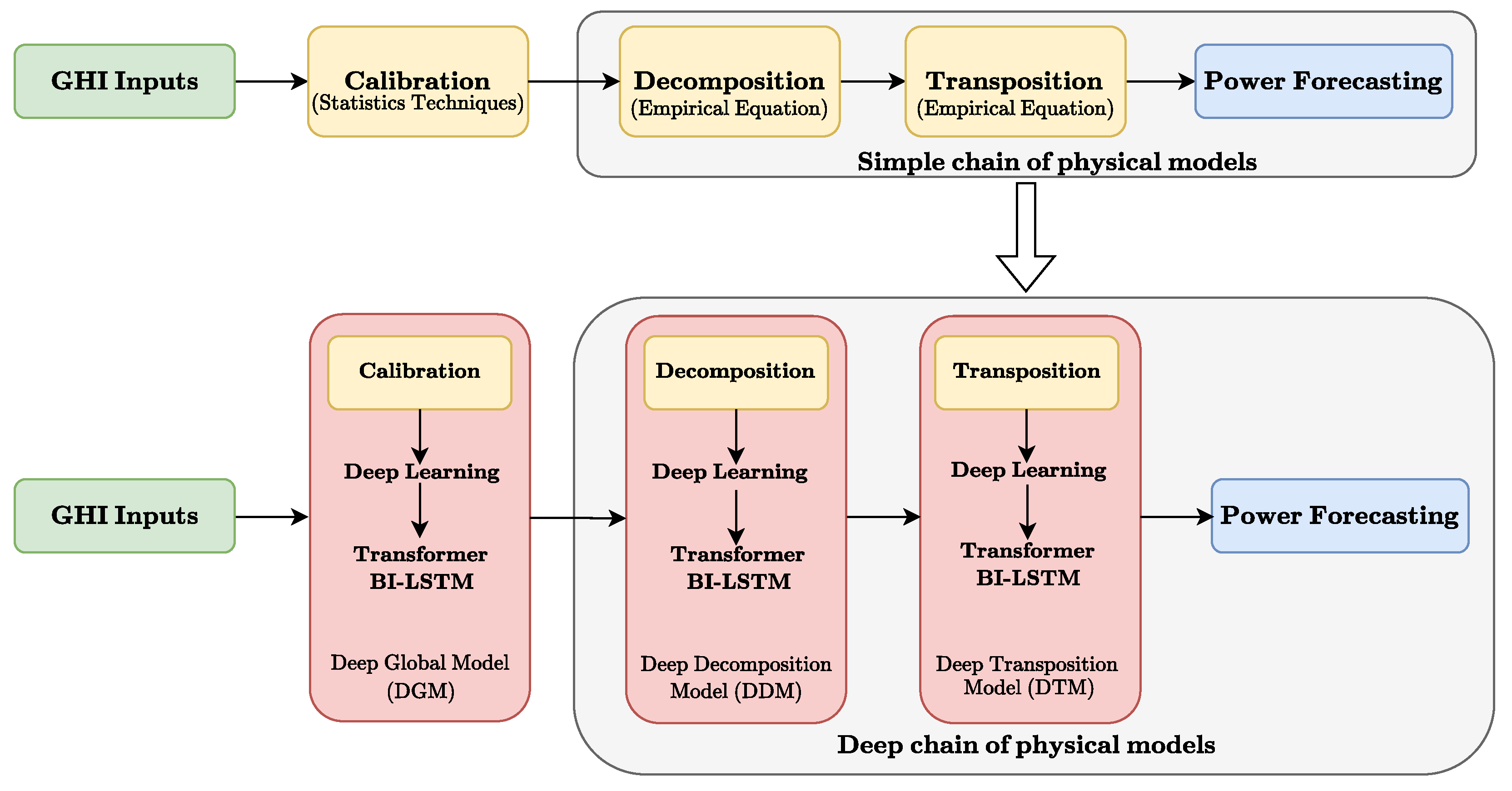
This study introduces a hybrid strategy to increase the accuracy of the intra-hour forecast of photovoltaic power generation. The proposal consists of the following elements: first, the data are post-processed to obtain more accurate GHI forecasts. Subsequently, a simple physical chain model is attached, which includes the processes of decomposition, transposition, and conversion from the plane of array irradiance Ipoa to power but with a deep learning approach as seen in Figure 2.
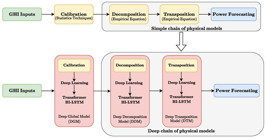
Figure 2.
Schematic explanation of our model: the standard methodology is represented above the arrow, and our proposal using the new Transformer Bi-LSTM model is represented below the same arrow.
The upper section represents the traditional physical chain model, where each stage (calibration, decomposition, and transposition) is performed using statistical techniques and empirical equations. The lower section presents the proposed deep learning-based approach, where each stage is replaced by a Transformer BI-LSTM model. The colours represent: green for the input Global Horizontal Irradiance (GHI), yellow for the steps in the traditional method, red for the deep learning models in the proposed method, and blue for the final power forecast.
It should be explicitly noted that in this article, no physical model of a photovoltaic module is implemented, as only an indirect approach is used, employing a deep learning model to model the transformation process from Ipoa to photovoltaic power. The latter is based on [23], where the author comments that the transformation steps between GHI and Ipoa are where the biggest errors occur. The proposed model inspired by existing research is used. This sequence of four steps is defined as a deep chain model. Each element of the chain is trained to replicate the function of each block of the traditional physical model chain. Later, we use the transfer learning technique, and all the models are concatenated to make the power forecast.
2.4. Features Engineering
Specific feature engineering is performed for each block in the chain to generate new features for model training.
2.4.1. Calibration of
Calibration of the data is crucial in obtaining more accurate predictions in solar power generation. The article [9] highlights that the technique should focus on fitting the magnitude and offset of the NWP data using Equation (1), where is the calibrated forecast, a and b are constants to find, and f is the original unadjusted forecast:
This process can be carried out using the MSE or MAE functions, thus improving the accuracy of global irradiance forecasts. It should be noted that for this process, optimizing by using RMSE or MSE is indistinct in that both functions already converge to the same minimum point, but the latter is used since it offers advantages in terms of the number of calculations to be carried out [24]. From this point forward, we will refer to the optimized calibration with MAE and MSE as and , respectively. And the most accurate GHI forecast between the values and its calibration (by MAE and MSE) will be called .
2.4.2. Physical Decomposition Models
In the physical chain model, the decomposition allows GHI to calculate its direct (DNI) and diffuse (DHI) components. Our study compares eight different models that estimate diffuse irradiance (see Table 5); with this component, we calculate it using the GHI closure equation (see Equation (2)). These models are selected for their relevance in [23]. We use data from weather stations to evaluate the accuracy of each model under different weather conditions to improve the DHI intra-hourly predictions in photovoltaic stations using . The model with the best fit will be referred to as :

Table 5.
Summary of tested physical decomposition models.
2.4.3. Physical Transposition Models
Irradiance transposition is key in solar power prediction [23] since it determines the solar irradiance that falls on the inclined surfaces of the panels or plane of array (POA). According to [35], the model from [36] is efficient for the transposition process, and although we do not have data to validate its accuracy, it is included due to its high performance in [21]. By applying the transposition model, we obtain the components defined in Equation (3) and for this investigation, this set of variables is called Ipoa. By convention, when these variables are derived from NWP, they are called . Same for LMD and ‘Best’. If we use the subscript GTI, we will be referring to :
where we have the following:
- : Total irradiance on the plane of array.
- : Direct normal irradiance component incident on the plane of the array.
- : Diffuse irradiance component from the sky incident on the plane of the array.
- : Diffuse irradiance component reflected from the ground incident on the plane of the array.
As there are no measurements in POA, the values will fulfill this function, and the sets and will be used as characteristics for training the chain model.
2.4.4. Model Architecture
Photovoltaic power prediction represents an intrinsic challenge that requires the conversion of various sequential variables into power forecasts. Due to the superior performance of the Transformer architecture [22], and LSTM [20], elements of this architecture have been incorporated as the basis for our proposal.
Based on the Transformer encoder from [37], our model simplifies the conventional structure by removing the positional coding and adding a linear layer with the same number of neurons as the number of input features. The model was chosen for its simplicity and the promising preliminary results obtained at the beginning of the research. This adaptation seeks to maintain computational efficiency without sacrificing performance in photovoltaic forecasts. In our design, the Transformer block acts as an encoder or feature generator, see Figure 3.

Figure 3.
Diagram of the proposed Transformer encoder.
The yellow block represents the Linear Layer that processes input features. The purple block corresponds to the Attention mechanism, which focuses on the most relevant parts of the input sequence. The red blocks denote Layer Normalization (Layer Norm), stabilising the learning process by normalizing inputs. Finally, the green section represents the Feed Forward Network (FFN) with a ReLU activation function, providing non-linear transformations to the data.
The output is fed into a bidirectional LSTM connected to an attention layer and a two-layer feed-forward network, followed by a linear layer of four neurons; the architecture is represented in Figure 4. The components of the model are colour-coded as follows: The blue block represents the Bi-LSTM layer, which processes the sequence in both temporal directions. The purple block represents the attention mechanism, highlighting the most relevant time steps. The green blocks indicate the feed-forward network with a ReLU activation, responsible for further transformation of the input data. Finally, the yellow blocks correspond to the output linear layer with ReLU activation, producing the forecasted power values.
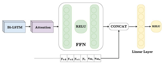
Figure 4.
Diagram of the proposed Bi-LSTM decoder, where each () represents the power measurement at (t), and the indices from -3 to 4 indicate measurements taken every 15 min, either before or after (t). For instance, () is the measurement taken 45 min before (t) and () is the measurement taken 60 min after (t).
This configuration is especially suitable for forecasting power production in the next hour and is fully illustrated in Figure 5.

Figure 5.
Simplified architecture of the proposed Transformer Bi-LSTM model.
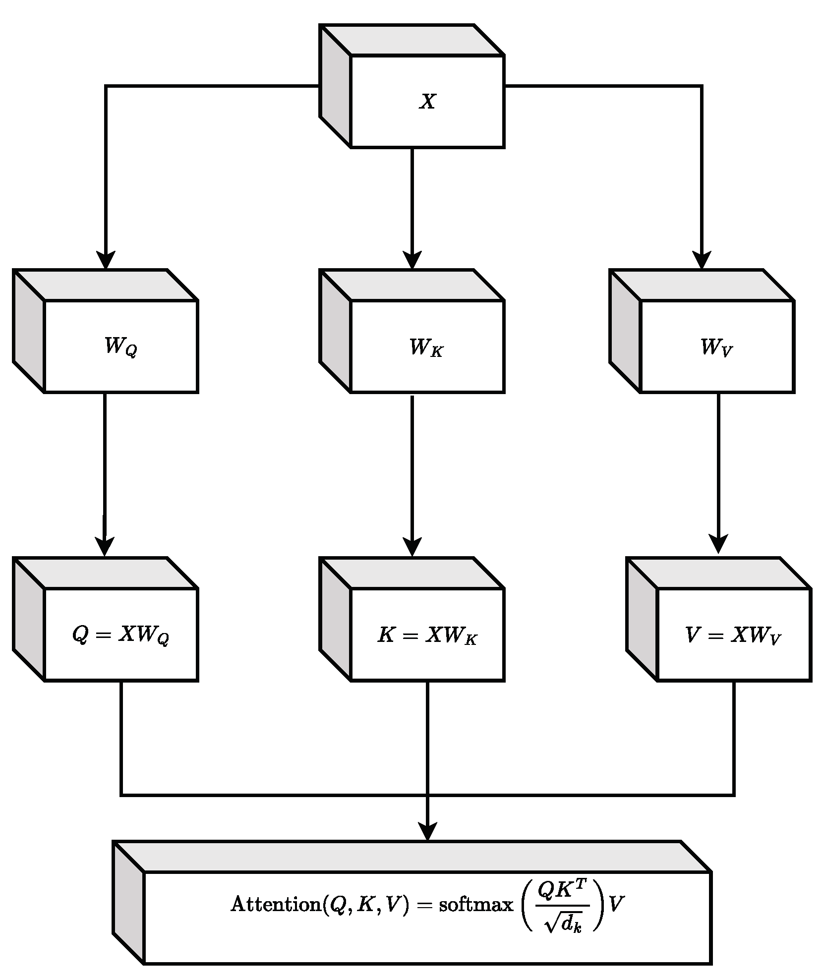
A crucial element in our proposal is the attention mechanism, which allows us to discern which parts of the input have the greatest relevance for the forecast. This mechanism is illustrated in Figure 6.
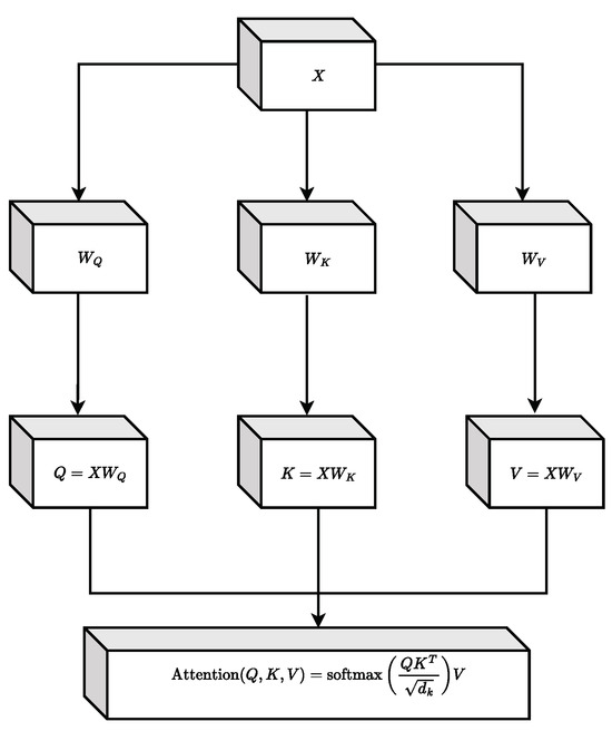
Figure 6.
Attention mechanism diagram.
2.4.5. Deep Chain Model
Our approach to deep chain models replaces each block in the physical chain with a Transformer Bi-LSTM model. Our proposed model works with the flow described by the following steps:
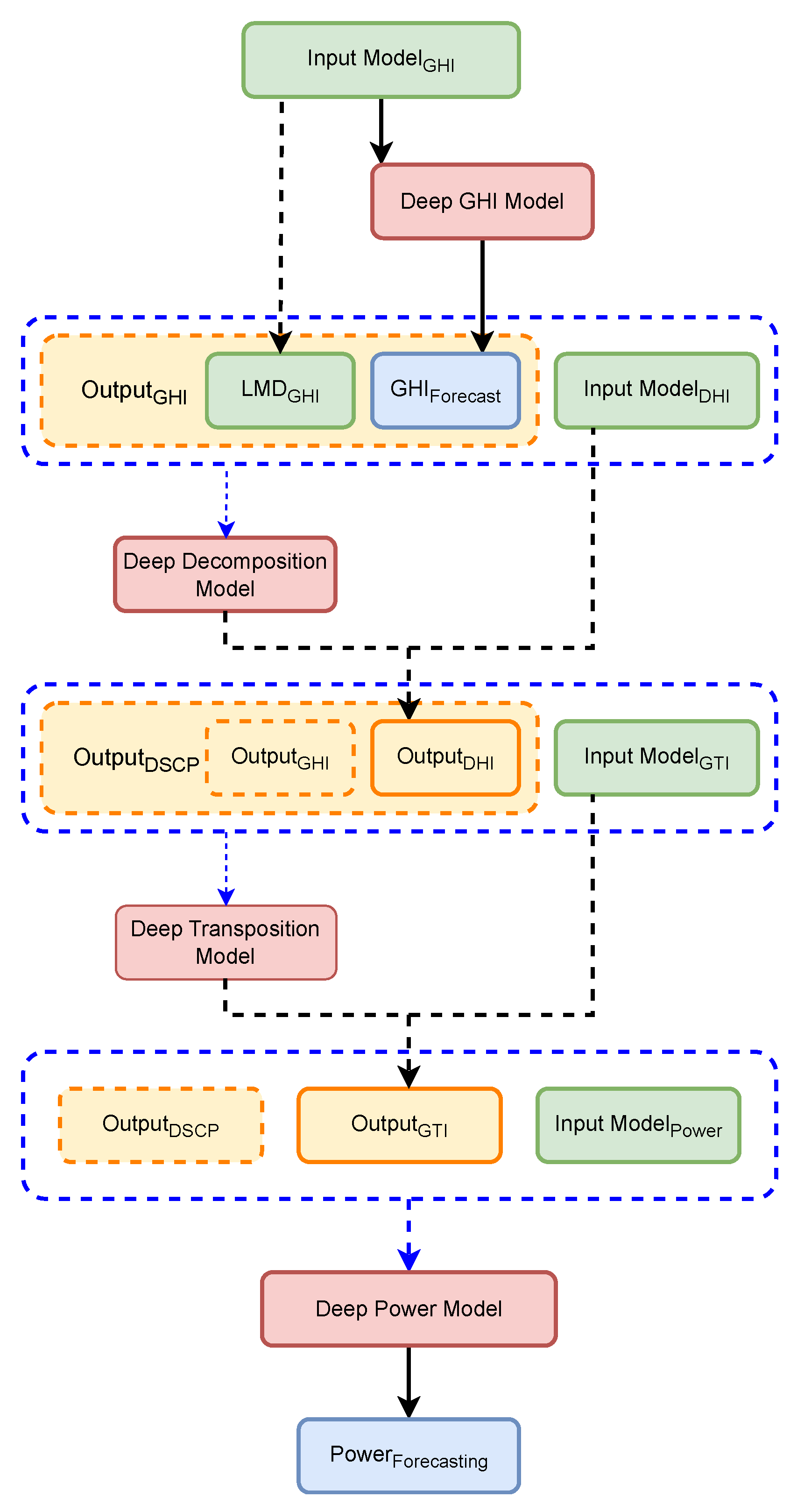
- First, from the inputs of GHI, besides the exogenous variables related primarily to solar positioning, once data go through a statistical calibration, they pass through the first instance of the Transformer Bi-LSTM architecture that we call the (DGM). The output from that first instance is a more accurate GHI forecast value, and it is called . At the same time, we use from the inputs of GHI the LMD version of this quantity, . Thus, a concatenation between the data and besides the exogenous variables is performed, creating a new vector that we call . These exogenous variables are described in greater detail in the following paragraphs.
- Then, , besides another variable like the exogenous variables -again-, passes through a decomposition model to obtain, from the GHI quantity, the best DHI values for forecasting. Now, we occupy a second instance of the Transformer Bi-LSTM model, which is used to learn the underlying physics of the decomposition process. This second instance is called the Deep Decomposition Model (DDC). At last, the result of the use of this second instance of the model is concatenated with the original data to form a new vector that we call . For future convenience, we define another new vector, called , as the concatenation between and .
- To take into account the tilt angle of the solar panels, both global irradiance and diffuse irradiance from have to go through a transposition method. Once the transposition over those irradiances is complete, the result of this process is the Global Tilted Irradiance (GTI) calculated by the third instance from the Transformer Bi-LSTM architecture, which we call the Deep Transposition Model (DTM). Then, those values are concatenated with the . This new concatenation creates a new vector called .
- Finally, using a concatenation between all the previous variables, and again beside the exogenous variables, and using a direct transformation method through a final instance from the Transformer Bi-LSTM architecture that we call the Deep Power Model (DPM), we perform the final power photovoltaic forecasting.
Figure 7 represents the proposed model. The green boxes denote the input models responsible for processing different irradiance and meteorological variables (GHI, DHI, GTI, Power). The orange boxes represent the concatenation of the previous hour’s measurements with the forecasted hour. The red boxes highlight the deep learning models that transform these inputs into more accurate predictions. The blue dashed lines represent the input-output framework, guiding the data through the stages and feeding the output from one model as input to the next.
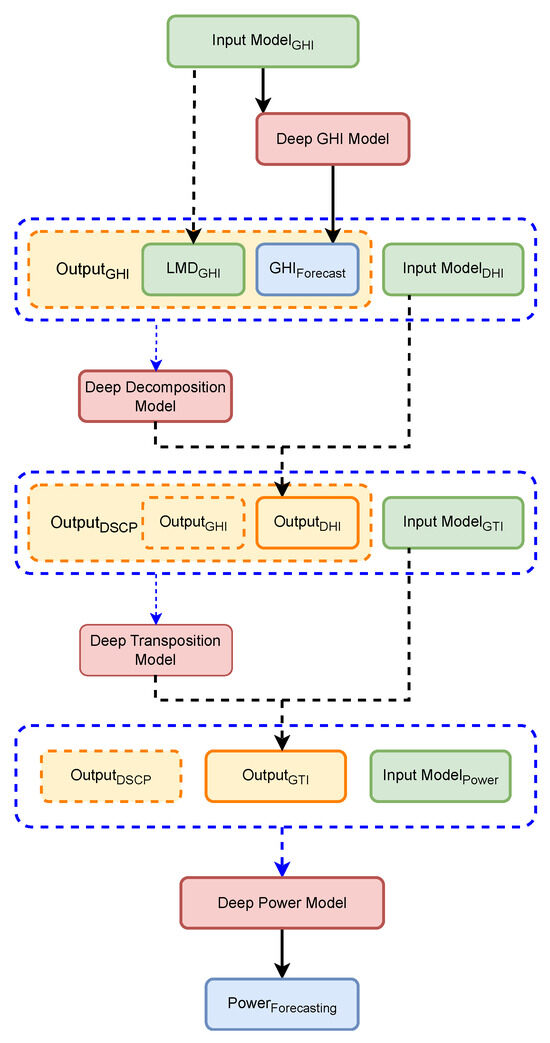
Figure 7.
Brief overview of our proposed chain model for power photovoltaic forecasting.
Although there are more complex approaches in the literature, our objective is to evaluate the effectiveness of the proposed architecture in a simplified context. Each model is trained independently, and specific data from the photovoltaic plant are integrated to improve forecast accuracy, exploring two methodologies: one direct and the other based on the proposed chain model.
The quality of the predictive model largely depends on the preparation and selection of data variables. The PVLIB library is used to extract active hours of solar irradiation, applying the Solar Position Algorithm (SPA) [38]. Anomalies are detected and corrected by cubic spline interpolation. We define abnormal data as zero power values when GHI is greater than 15 W/m2.
To structure the time series, key parameters are established: window size timestamp is initially set somewhat arbitrarily, serving as a starting point to facilitate data handling. Forecast horizon timestamp is chosen to align and compare with the methodologies used in the referenced papers [21,22]: number of input variables , amount of input metadata , and number of previous chain blocks . It should be remembered that each timestamp is equivalent to 15 min, so considering 4 timestamps would correspond to one hour. These parameters are consolidated into the input vector with length N given by Equation (4) and illustrated in Figure 8 and Figure 9:
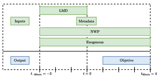
Figure 8.
Framework of the data preparation process.

Figure 9.
General order of the inputs for the Transformer Bi-LSTM model. The symbol * represents data that are not added to every block in the chain.
The green boxes represent the various inputs and exogenous variables used in the forecasting model, including Local Measurement Data (LMD), Metadata, Numerical Weather Prediction (NWP), and exogenous factors such as solar position. The blue boxes indicate the outputs of the model’s prediction results. The timeline marked from min to min shows the temporal framework, where data is used for both historical input and future prediction targets.
The selection of variables depends on their significance for forecasting the horizontal irradiance, the plane of the array, and the generation of photovoltaic power. We have chosen to incorporate the exogenous variables and across all proposed models, as they provide a comprehensive description of solar movement throughout the day. It is crucial to understand that the angle denotes the inclination between a point in the sky and the vertical over a specific location, while the angle is the measure between a point on the horizontal plane and a fixed reference, usually geographic North. These variables are obtained using the SPA algorithm. Additionally, metadata such as the inclination angle of the solar panel are included to improve the accuracy of the model.
Table 6 summarizes all these variables, which are tailored according to the specific segment of the prediction chain.

Table 6.
Summary of variables by model and methodology.
Stations 0, 1, 2, 3, 4, 5, and 8 are chosen for the formation and evaluation of the blocks of the model chain, as well as the calibration of the variable . This selection is based on previous studies to facilitate comparisons with [21,22].
The measurements of each station are sorted chronologically. Three days are assigned for training, one for validation and one for testing, for each block of five days. This distribution guarantees a climatic balance in the evaluations and is consistent with previous studies [22]. The final sizes of the datasets are 55,280, 18,216, and 18,206 for training, testing, and validation, respectively.
To evaluate the effectiveness of this methodological proposal, a set of metrics commonly adopted in research on photovoltaic power generation forecasts is used: these are specifically MAE, RMSE, and . Finally, the implementation is performed on a system with an Intel i7, 16 GB of RAM and an NVIDIA GTX1660-TI GPU. Python (v3.10) and PyTorch (v2.0) [39] are used as the framework with a batch size of 1000. The Adam optimizer is adopted with an initial learning rate of 0.01 and a learning rate scheduler that reduces it by a factor of 0.10 every 80 epochs. After 120 training epochs, satisfactory convergence is achieved without overfitting. The loss function L1Loss (MAE) is chosen, given its suitability for predictive tasks. The training takes approximately 10 min.
3. Results
To evaluate the performance of the models, the following metrics are used:
where () represents the observed values, () are the predicted values by the model, () is the mean of the observed values, and (n) is the total number of observations. The MAE measures the average absolute error between the predictions and the actual values. The MSE calculates the average of the squared differences between the predicted and observed values, placing more weight on larger errors. The RMSE is the square root of the MSE, providing a metric in the same units as the original data. The () measures the proportion of variance in the observed data that is predictable from the independent variables, providing an indication of the goodness of fit.
3.1. NWP Data Calibration
Initially, the is calibrated to mitigate systematic biases and analyze the effectiveness of different calibration strategies where MAE and MSE functions are used to achieve this objective. The calibration is carried out individually for each station, to take into account local climatic conditions. The training and validation data are used for calibration, and it is evaluated with the test set. The Minimize function of the Scipy library is used for optimization with MAE, following the approach of [24] for MSE.
The results, presented in Table 7, suggest that calibration using MAE slightly outperforms that achieved with MSE in terms of MAE but shows similar performance in RMSE. It is noticed that stations 4 and 5 exhibited lower performance, suggesting quality issues in their measurements or forecasts. In general, calibration is most effective when the raw forecasts are of high quality. As a recommendation, it is essential to identify stations with high and low quality raw forecasts before applying the general calibration. This allows the evaluation of whether calibration offers a significant improvement in forecast accuracy.

Table 7.
Calibration results of . RMSE and MAE are measured in [W/m2].
3.2. Irradiance Decomposition
The results presented in Table 8 indicate that the Skartveit model surpasses the in accuracy. In the MAE and RMSE metrics, models such as Engerer, DISC and Dirint are inferior to , so they are discarded from all analysis. The Skartveit model shows an average MAE of 98 [W/m2] and an of 0.41, notably outperforming the outcomes of , which only obtained a of 0.12.

Table 8.
Results of physical decomposition models with reference. RMSE and MAE are measured in [W/m2], and is unitless.
Although the Skartveit model does not consistently improve the forecast across all seasons, on average, it demonstrates significant improvements in the MAE, RMSE, and metrics. Therefore, Skartveit is selected as the for future testing in photovoltaic power forecasting models.
3.3. GHI Deep Model
The Transformer Bi-LSTM model applied on the GHI block gives encouraging performance results under various conditions. When compared to the base error of , which has a MAE of 120 [W/m2] and a RMSE of 175 [W/m2], two methods are implemented. In the first method, the variable is employed, and in the second one, is added. It should be remembered that the variables and are used as the basis for all models. The results are listed in Table 9.

Table 9.
Results of deep GHI model block. RMSE and MAE are measured in [W/m2], and is unitless.
Both methods achieve an average MAE of 54, an RMSE of 105, and an of 0.88. However, the second method produces better results in a greater number of plants, leading us to select it for the subsequent steps. These models substantially improve accuracy at all stations compared to , reducing on average the MAE and RMSE by , and increasing a , respectively.
In addition to the above, it can be seen that the inclusion of calibration has a marginal impact on the precision of the forecasts but in stations 4 and 5, the model demonstrates its effectiveness by significantly reducing the MAE and RMSE errors. Although the calibration provides minimal improvements in MAE and slightly worsens the RMSE, most of the improvement comes from using the Transformer Bi-LSTM model.
In summary, this model is effective in improving the accuracy of GHI forecasts, especially at stations with poor initial predictions.
3.4. Irradiance Decomposition Model
Like the GHI model, the Transformer Bi-LSTM model for the decomposition process shows a positive trend in its performance.The MAE errors of 118 [W/m2], an RMSE of 176 [W/m2], and an of 0.12, obtained with are taken as a reference. As a reminder, three methodologies of two types are tested: the direct one, which does not use the output of the GHI model, and the indirect one which uses a chain model. Within the latter, two sets are occupied, where their main difference is the use of the Skartveit decomposition model.
The results, presented in Table 10, demonstrate that both the direct forecasting method and the chain model significantly improve the precision in all cases, particularly at stations 0, 1, and 2. It is important to note that the error at station 3 is significantly reduced, with decrements of approximately .

Table 10.
Results of Deep Decomposition Model block. RMSE and MAE are measured in [W/m2], and is unitless.
The results demonstrate that the Transformer Bi-LSTM model is key to improving forecast accuracy. Incorporating the GHI block and the Skartveit model as additional variables shows a marginal but positive impact on the prediction accuracy. Accuracy is improved at all stations: MAE is reduced to 30 W/m2, RMSE to 58 W/m2, and is increased to .
3.5. Irradiance Transposition Model
The conversion of GHI a GTI stands out as a crucial element for the accuracy of the power forecast [21]. This evidence is also supported by the results of Table 11, where the estimation of power is presented with the variables and . This underlines the need to implement and optimize this specific phase of the physical chain. Particularly for this block, the inclination angle of the photovoltaic module is added in all the tests carried out due to its importance.

Table 11.
Training results of Transformer Bi-LSTM for photovoltaic power estimation with GHI derived from sensors and . RMSE and MAE are measured in , and is unitless.
The metrics in Table 12 demonstrate that the chain model trained with the sets and improves precision, but there is still room for optimization, especially considering that irradiance measurements are not available in the plane of the modules.

Table 12.
Results of deep transposition model block. RMSE and MAE are measured in [W/m2], and is unitless.
3.6. Direct Method
In our approach, the deep power forecasting model using the direct method allows us to exploit the differences with the indirect method proposed in power forecasting. The data in Table 11 allow us to estimate an ideal performance that could have the direct or indirect methodology of having GHI and GTI forecasts with zero error, which further underlines the importance of these variables.
Table 13 shows that the model trained with the variables and Skartveit obtain an MAE of 0.896 MW, RMSE of 1.677 MW and of , representing the “optimal case”. Furthermore, different combinations of variables barely affect the metrics, but all outperform conventional methods, validating the effectiveness of the direct method. Contrasting the errors by station shows considerable deviations in stations 4 and 5 as in the results of the GHI block, which suggests problems with the pyranometer or, failing that, with the NWP forecasts. Station 0, however, validates the great effectiveness of the Transformer Bi-LSTM model in improving forecasts.

Table 13.
Results of direct method to power forecast. RMSE and MAE are measured in , and is unitless.
3.7. Deep Chain Model
Table 14 shows that the model trained with and slightly outperforms the best direct method model in all metrics, although without a significant improvement compared to the direct method. However, this method allows for a modularization of errors, which is crucial for future improvements. The deep chain model presents a more integrated strategy for power prediction.

Table 14.
Results of deep chain model method to power forecast. RMSE and MAE are measured in , and is unitless.
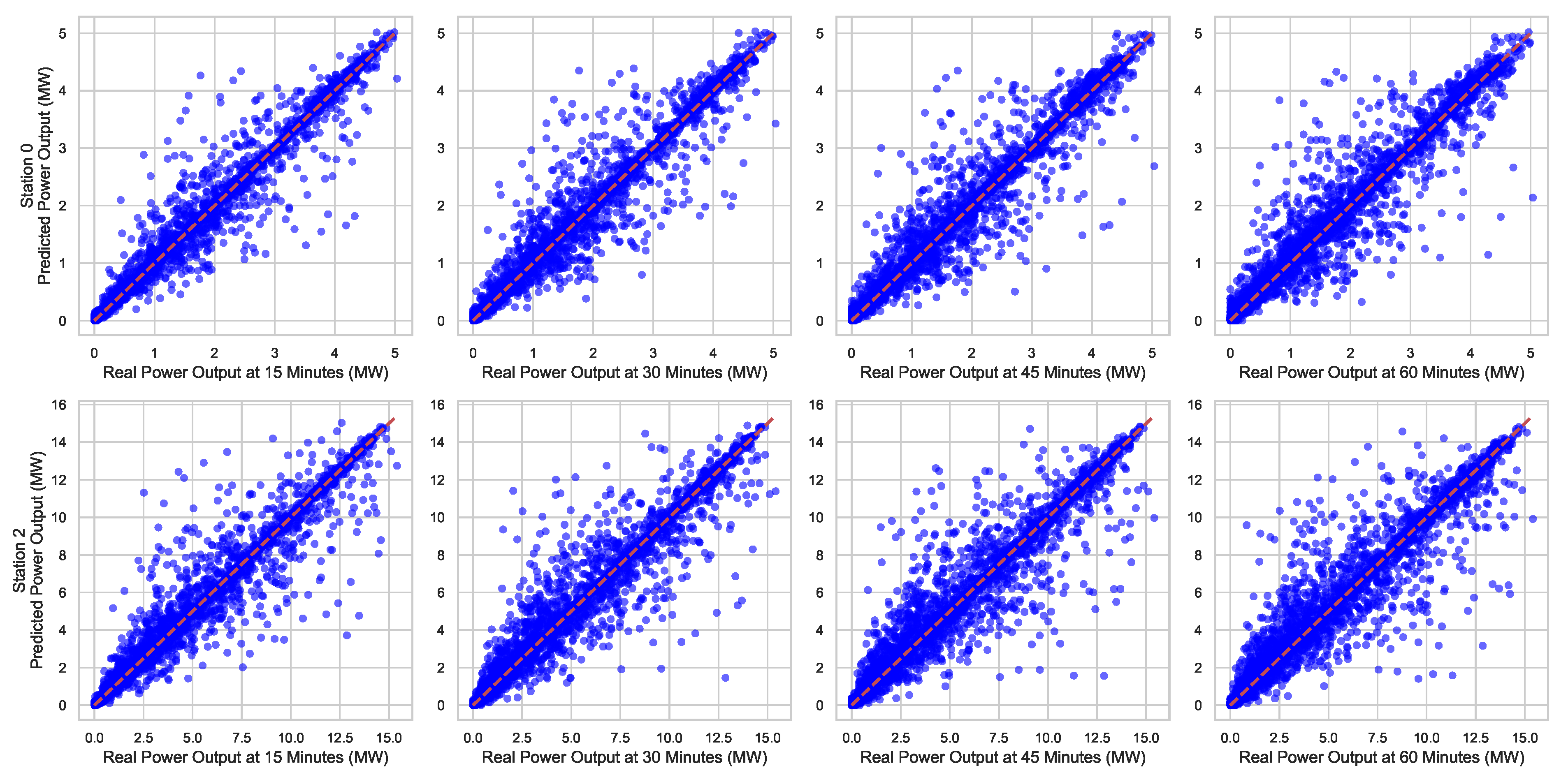
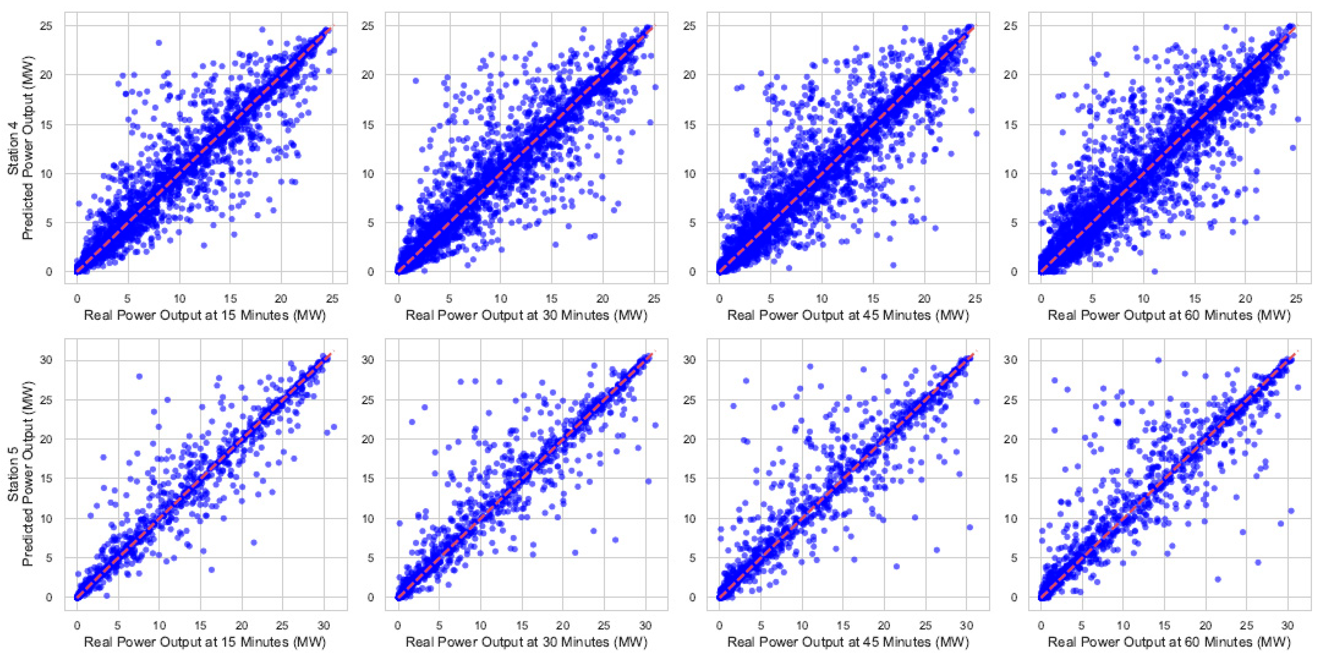
Figure 10 and Figure 11 show the graphical representation of the best and worst forecasting results, respectively, using the best model found. The scatter plots in each figure compare the actual versus predicted power values for different stations using the deep chain model method. Each plot corresponds to one station, with the x-axis representing the observed power and the y-axis representing the predicted power. The diagonal line indicates the ideal 1:1 relationship.
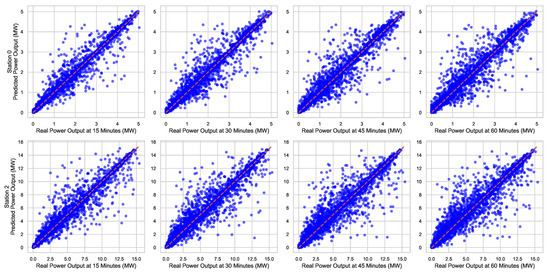
Figure 10.
Relationship between observed and predicted power output for different stations and prediction horizons for stations with better results.
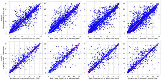
Figure 11.
Relationship between observed and predicted power output for different stations and prediction horizons for stations with worst results.
Each row in the figures represents a measurement in one station (or plant), while each column corresponds to a prediction horizon in 15 min increments, starting from 15 min up to 60 min. The main diagonal in each plot indicates the line of identity, where the predicted values perfectly match the observed values.
When compared with previous results, it is evident that the deep chain model benefits from each stage of the prediction process, although it shows an inherent error, coming from the first block and propagating through the others, which cannot be eliminated with this strategy.
It is seen that among the results, there is no significant difference between the different training datasets used, although there is still room for more tests with other variables, whether they are sensor measurements or calculated variables. Despite the above, this study represents a considerable advance in improving the accuracy of photovoltaic power predictions, and given the innovative use of the proposed Transformer Bi-LSTM architecture, it lays a solid foundation for future research in the field.
4. Discussion
The challenge of predicting solar power generation demands advanced approaches. In this context, the present study uses modern deep modeling techniques and, through data adjustments, exhibits promising results according to Table 15, where it can be seen that our model is superior to the state-of-the-art results in most cases of photovoltaic stations.

Table 15.
Comparison of obtained results with those present in the state of the art. RMSE and MAE are measured in .
The errors of stations 4 and 5 have a particular behavior, although in each block they are the stations that presented the greatest improvements in the forecasts, as well as being the stations with the lowest performance compared to the other stations. In Section 3.7, a possible reason for this particularity is already mentioned, but without more detail about the state and maintenance of the sensors, nothing conclusive can be stated.
In any case, despite these possible errors, we see that the proposed model gives less priority to these stations to adjust to the rest of the stations. The above could mean that the model is overfitting to these plants, so we apply the latter on stations not seen in the training phase, the results of which are shown in Table 16. It is seen that the errors are by the results of the other stations, demonstrating that the good results of the proposed module do not correspond to overfitting, but rather derive from a correct generalization.

Table 16.
Results of the deep chain model in stations not present during training. RMSE and MAE are measured in , and is unitless.
Our proposed deep chain model outperforms state-of-the-art performance metrics, especially at stations with less accurate forecasts, highlighting the effectiveness of the Transformer Bi-LSTM in mitigating prediction errors. However, the deep chain model also faces a major challenge, the main being susceptible to cumulative errors.
Although the feature engineering process helps by improving the forecasts of the chain blocks corresponding to GHI and decomposition, this does not have a great impact on the final intra-hour power forecasting, with the proposed model being mainly responsible for the good results.
It should be remembered that this methodology has been developed without irradiance measurements in the array plane, so there is still a large margin for optimization in the transposition block, although most of the error comes from the NWP forecasts, which agrees with what is seen in the literature.
In summary, both the deep chain model and the direct approach offer benefits and limitations, and the selection between them will depend on the particular requirements of the project and the available resources.
5. Conclusions
Through this study, we introduced an innovative hybrid methodology for photovoltaic power generation forecasting using a Transformer Bi-LSTM model; for the calibration block, it has been demonstrated to be superior in comparison with the traditional calibration, in terms of forecasting accuracy. Despite the fact that the preprocessing of the data does not significantly increase the accuracy of the model, the methodology of direct forecasting offers some equilibrium between precision and efficiency at the time of the development, although the chain model offers more details in the process of irradiance transformation into photovoltaic power. In particular, the deep chain model has proven to be superior compared to conventional prediction methods, achieving a reduction in MAE of 24% MAE and RMSE 4%, in comparison to the best results of the state of the art. This has allowed achieving MAE values as low as 0.894 [MW] and RMSE of 1.669 [MW], which represents a significant improvement over reference models in the literature.
Although the results are promising, it is essential to test the model in real-field scenarios to evaluate its accuracy under real conditions. This evaluation would pave the way for implementing a fault detection system that triggers alerts when model predictions deviate significantly from actual measured values. This would improve the operation and maintenance of photovoltaic plants, allowing a significant reduction in operating costs.
For future research, we propose exploring more advanced neural model architectures, optimizing specific components, and applying our methodology to larger datasets, such as the California-based dataset mentioned earlier. These improvements will not only enhance the accuracy of photovoltaic energy forecasts but also offer deeper insights into the overall field of renewable energy prediction. Moreover, given that our approach integrates physical models with deep learning, future work could focus on refining this hybrid method. Potential directions include tuning trainable physical equations within neural networks and embedding these equations into the loss function, replicating the Physics-Informed Neural Networks methodology, further advancing the interpretability and performance of predictive models in photovoltaic energy.
Author Contributions
Conceptualization, G.F. and J.R.; methodology, J.R.; software, J.R.; validation, G.G., E.F. and M.L.; formal analysis, J.R.; investigation, J.R. and M.L.; resources, G.F., E.F. and S.D.-C.; data curation, J.R. and M.L.; writing—original draft preparation, J.R. and G.G.; writing—review and editing, G.G. and E.F.; visualization, J.R.; supervision, G.F.; project administration, G.F.; funding acquisition, E.F., G.G and S.D.-C. All authors have read and agreed to the published version of the manuscript.
Funding
This research was supported, in part, by the Chilean Research and Development Agency (ANID) under Project FONDECYT 1191188. The Ministry of Science and Innovation of Spain under Project PID2022-137680OB-C32. The Agencia Estatal de Investigación (AEI) under Project PID2022-139187OB-I00.
Data Availability Statement
The original contributions presented in the study are included in the article, further inquiries can be directed to the corresponding author.
Conflicts of Interest
The authors declare no conflict of interest.
References
- Barhmi, K.; Heynen, C.; Golroodbari, S.; van Sark, W. A Review of Solar Forecasting Techniques and the Role of Artificial Intelligence. Solar 2024, 4, 99–135. [Google Scholar] [CrossRef]
- Sengupta, M.; Habte, A.; Wilbert, S.; Gueymard, C.; Remund, J. Best Practices Handbook for the Collection and Use of Solar Resource Data for Solar Energy Applications; Technical report; National Renewable Energy Lab (NREL): Golden, CO, USA, 2021.
- Liu, H.; Gao, Q.; Ma, P. Photovoltaic generation power prediction research based on high quality context ontology and gated recurrent neural network. Sustain. Energy Technol. Assessments 2021, 45, 101191. [Google Scholar] [CrossRef]
- Sperati, S.; Alessandrini, S.; Pinson, P.; Kariniotakis, G. The “weather intelligence for renewable energies” benchmarking exercise on short-term forecasting of wind and solar power generation. Energies 2015, 8, 9594–9619. [Google Scholar] [CrossRef]
- Keisang, K.; Bader, T.; Samikannu, R. Review of Operation and Maintenance Methodologies for Solar Photovoltaic Microgrids. Front. Energy Res. 2021, 9, 730230. [Google Scholar] [CrossRef]
- Qureshi, M.S.; Umar, S.; Nawaz, M.U. Machine Learning for Predictive Maintenance in Solar Farms. Int. J. Adv. Eng. Technol. Innov. 2024, 1, 27–49. [Google Scholar]
- Ulbricht, R.; Fischer, U.; Lehner, W.; Donker, H. First steps towards a systematical optimized strategy for solar energy supply forecasting. In Proceedings of the European Conference on Machine Learning and Principles and Practice of Knowledge Discovery in Databases (ECMLPKDD 2013), Prague, Czech Republic, 23–27 September 2013; Volume 2327, pp. 1–12. [Google Scholar]
- Yao, T.; Wang, J.; Wu, H.; Zhang, P.; Li, S.; Wang, Y.; Chi, X.; Shi, M. A photovoltaic power output dataset: Multi-source photovoltaic power output dataset with Python toolkit. Sol. Energy 2021, 230, 122–130. [Google Scholar] [CrossRef]
- Mayer, M.J.; Yang, D. Probabilistic photovoltaic power forecasting using a calibrated ensemble of model chains. Renew. Sustain. Energy Rev. 2022, 168, 112821. [Google Scholar] [CrossRef]
- Balaraman, K. Development of a day-ahead solar power forecasting model chain for a 250 MW PV park in India. Int. J. Ind. Chem. 2023, 14, 1–15. [Google Scholar]
- Yang, D.; Wang, W.; Xia, X. A concise overview on solar resource assessment and forecasting. Adv. Atmos. Sci. 2022, 39, 1239–1251. [Google Scholar] [CrossRef]
- Pan, S.J.; Yang, Q. A survey on transfer learning. IEEE Trans. Knowl. Data Eng. 2009, 22, 1345–1359. [Google Scholar] [CrossRef]
- Nespoli, A.; Ogliari, E.; Leva, S.; Massi Pavan, A.; Mellit, A.; Lughi, V.; Dolara, A. Day-Ahead Photovoltaic Forecasting: A Comparison of the Most Effective Techniques. Energies 2019, 12, 1621. [Google Scholar] [CrossRef]
- Yao, T.; Wang, J.; Wu, H.; Zhang, P.; Li, S.; Wang, Y.; Chi, X.; Shi, M. PVOD v1.0 : A Photovoltaic Power Output Dataset; Science Data Bank: Beijing, China, 2021. [Google Scholar] [CrossRef]
- Pombo, D.V. The SOLETE dataset, 2023. Retrieved from DTU-Data. Available online: https://figshare.com/articles/dataset/The_SOLETE_dataset/17040767 (accessed on 21 June 2024).
- Bob05757. Renewable Energy Generation Input Feature Variables Analysis. 2024. Available online: https://github.com/Bob05757/Renewable-energy-generation-input-feature-variables-analysis (accessed on 21 September 2024).
- Pedro, H.T.; Larson, D.P.; Coimbra, C.F. A Comprehensive Dataset for the Accelerated Development and Benchmarking of Solar Forecasting Methods. J. Renew. Sustain. Energy 2019, 11, 036102. [Google Scholar] [CrossRef]
- Pombo, D.V.; Gehrke, O.; Bindner, H.W. SOLETE, a 15-month long holistic dataset including: Meteorology, co-located wind and solar PV power from Denmark with various resolutions. Data Brief 2022, 42, 108046. [Google Scholar] [CrossRef] [PubMed]
- Chen, Y.; Xu, J. Solar and wind power data from the Chinese state grid renewable energy generation forecasting competition. Sci. Data 2022, 9, 577. [Google Scholar] [CrossRef]
- Chen, X.; Wu, Y.; He, X. Long Short-Term Memory Network PV Power Prediction Incorporating Extreme Extreme Gradient Boosting Algorithm. In Proceedings of the 2022 12th International Conference on Power and Energy Systems (ICPES), Guangzhou, China, 23–25 December 2022; pp. 821–825. [Google Scholar]
- Wang, K.; Dou, W.; Wei, H.; Zhang, K. Intra-hour PV Power Forecasting based on Multi-source Data and PSC-SVR Model. In Proceedings of the 2022 41st Chinese Control Conference (CCC), Hefei, China, 25–27 July 2022; pp. 3202–3207. [Google Scholar]
- Yao, T.; Wang, J.; Wang, Y.; Zhang, P.; Cao, H.; Chi, X.; Shi, M. Very short-term forecasting of distributed PV power using GSTANN. CSEE J. Power Energy Syst. 2022, 10, 1491–1501. [Google Scholar]
- Mayer, M.J.; Gróf, G. Extensive comparison of physical models for photovoltaic power forecasting. Appl. Energy 2021, 283, 116239. [Google Scholar] [CrossRef]
- Mayer, M.J.; Yang, D. Calibration of deterministic NWP forecasts and its impact on verification. Int. J. Forecast. 2023, 39, 981–991. [Google Scholar] [CrossRef]
- Erbs, D.; Klein, S.; Duffie, J. Estimation of the diffuse radiation fraction for hourly, daily and monthly-average global radiation. Sol. Energy 1982, 28, 293–302. [Google Scholar] [CrossRef]
- Skartveit, A.; Olseth, J.A. A model for the diffuse fraction of hourly global radiation. Sol. Energy 1987, 38, 271–274. [Google Scholar] [CrossRef]
- Bird, R.E.; Hulstrom, R.L. Simplified Clear Sky Model for Direct and Diffuse Insolation on horizontal Surfaces; Technical Report; Solar Energy Research Institute (SERI): Golden, CO, USA, 1981. [Google Scholar]
- Gueymard, C.A. Direct solar transmittance and irradiance predictions with broadband models. Part I: Detailed theoretical performance assessment. Sol. Energy 2003, 74, 355–379. [Google Scholar] [CrossRef]
- Ineichen, P.; Perez, R.; Seal, R.; Maxwell, E.; Zalenka, A. Dynamic global-to-direct irradiance conversion models. Ashrae Trans. 1992, 98, 354–369. [Google Scholar]
- Perez, R.; Ineichen, P.; Moore, K.; Kmiecik, M.; Chain, C.; George, R.; Vignola, F. A new operational model for satellite-derived irradiances: Description and validation. Sol. Energy 2002, 73, 307–317. [Google Scholar] [CrossRef]
- Ridley, B.; Boland, J.; Lauret, P. Modelling of diffuse solar fraction with multiple predictors. Renew. Energy 2010, 35, 478–483. [Google Scholar] [CrossRef]
- Engerer, N. Min resolution estimates of the diffuse fraction of global irradiance for southeastern Australia. Sol. Energy 2015, 116, 215–237. [Google Scholar] [CrossRef]
- Bright, J.M.; Engerer, N.A. Engerer2: Global re-parameterisation, update, and validation of an irradiance separation model at different temporal resolutions. J. Renew. Sustain. Energy 2019, 11, 033701. [Google Scholar] [CrossRef]
- Abreu, E.F.; Canhoto, P.; Costa, M.J. Prediction of diffuse horizontal irradiance using a new climate zone model. Renew. Sustain. Energy Rev. 2019, 110, 28–42. [Google Scholar] [CrossRef]
- Yang, D. Solar radiation on inclined surfaces: Corrections and benchmarks. Sol. Energy 2016, 136, 288–302. [Google Scholar] [CrossRef]
- Perez, R.; Ineichen, P.; Seals, R.; Michalsky, J.; Stewart, R. Modeling daylight availability and irradiance components from direct and global irradiance. Sol. Energy 1990, 44, 271–289. [Google Scholar] [CrossRef]
- Vaswani, A.; Shazeer, N.; Parmar, N.; Uszkoreit, J.; Jones, L.; Gomez, A.N.; Kaiser, Ł.; Polosukhin, I. Attention is all you need. In Proceedings of the 31st Conference on Neural Information Processing Systems (NIPS 2017), Long Beach, CA, USA, 4–9 December 2017; Volume 30. [Google Scholar]
- Reda, I.; Andreas, A. Solar position algorithm for solar radiation applications. Sol. Energy 2004, 76, 577–589. [Google Scholar] [CrossRef]
- Imambi, S.; Prakash, K.B.; Kanagachidambaresan, G. PyTorch. Programming with TensorFlow: Solution for Edge Computing Applications; Springer: Berlin/Heidelberg, Germany, 2021; pp. 87–104. [Google Scholar]
Disclaimer/Publisher’s Note: The statements, opinions and data contained in all publications are solely those of the individual author(s) and contributor(s) and not of MDPI and/or the editor(s). MDPI and/or the editor(s) disclaim responsibility for any injury to people or property resulting from any ideas, methods, instructions or products referred to in the content. |
© 2024 by the authors. Licensee MDPI, Basel, Switzerland. This article is an open access article distributed under the terms and conditions of the Creative Commons Attribution (CC BY) license (https://creativecommons.org/licenses/by/4.0/).


