The Porcupine Measure for Comparing the Performance of Multi-Objective Optimization Algorithms

Abstract

In spite of being introduced over twenty-five years ago, Fonseca and Fleming’s attainment surfaces have not been widely used. This article investigates some of the shortcomings that may have led to the lack of adoption of this performance measure. The quantitative measure based on attainment surfaces, introduced by Knowles and Corne, is analyzed. The analysis shows that the results obtained by the Knowles and Corne approach are influenced (biased) by the shape of the attainment surface. Improvements to the Knowles and Corne approach for bi-objective Pareto-optimal front (POF) comparisons are proposed. Furthermore, assuming M objective functions, an M-dimensional attainment-surface-based quantitative measure, named the porcupine measure, is proposed for comparing the performance of multi-objective optimization algorithms. A computationally optimized version of the porcupine measure is presented and empirically analyzed.

1. Introduction

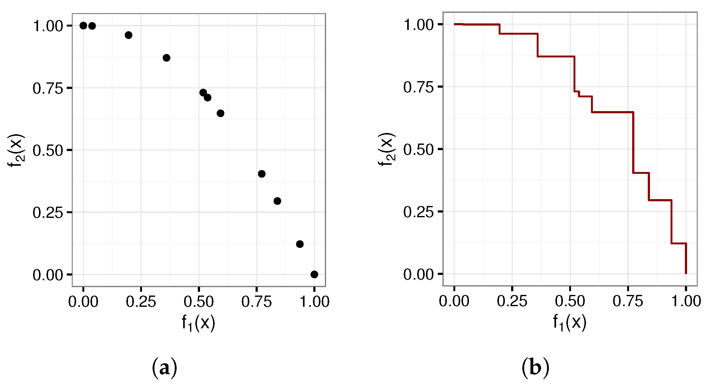
First introduced by Fonseca and Fleming [1], attainment surfaces provide researchers in multi-objective optimization with a means to accurately visualize the region dominated by a Pareto-optimal front (POF). In many studies, approximated Pareto optimal fronts (POFs) are shown by joining the non-dominated solutions using a curve. Fonseca and Fleming reasoned that it is not correct to use a curve to join these non-dominated solutions. The use of a curve creates a false impression that intermediate solutions exist between any two non-dominated solutions. In reality, there is no guarantee that any intermediate solutions exist. Fonseca and Fleming suggested that, instead of a curve, the non-dominated solutions can be used to create an envelope that separates the dominated and non-dominated spaces. The envelope formed by the non-dominated solutions is referred to as an attainment surface.

Despite being proposed in 1995, attainment surfaces have not seen wide use in the comparison of multi-objective algorithms (MOAs). Instead, the well-known hypervolume [2,3], inverted generational distance [4,5] and its improvements [6], and spread [7] measures are frequently used to quantify and to compare the quality of approximated POFs. This study provides an analysis of the shortcomings of attainment surfaces as a multi-objective performance measure. Specifically, the attainment-surface-based measure proposed by Knowles and Corne [8] is analyzed. Improvements to Knowles and Corne’s approach for bi-objective optimization problems are developed and analyzed in this paper. Additionally, an M-dimensional (where M is the number of objectives) attainment-surface-based quantitative measure, named the porcupine measure, is proposed and analyzed.

The porcupine measure provides a way to quantify the ratio of the Pareto front when one algorithm performs statistically significantly better than another algorithm. The objective of this paper is to introduce this new attainment-surface-based measure and to illustrate its applicability. For this purpose, the measure is applied to compare the performance of arbitrary selected MOAs on a set of multi-objective optimization benchmark problems. Note that the focus is not on an extensive comparison of multi-objective algorithms but rather on validating the use of the porcupine measure as a statistically sound mechanism to compare MOAs.

The remainder of this paper is organized as follows. Section 2 introduces multi-objective optimization along with the definitions used throughout this paper. Section 3 presents the background and related work. Next, 2-dimensional attainment surfaces are introduced in Section 4, followed by a weighted approach to produce attainment surfaces in Section 5. The generalization to M dimensions is provided in Section 6. Finally, the conclusions are given in Section 7.

2. Definitions

Without loss of generality, assuming minimization, a multi-objective optimization problem (MOP) with M objectives is of the form

$$\mathrm{m}\mathrm{i}\mathrm{n}\mathrm{i}\mathrm{m}\mathrm{i}\mathrm{z}\mathrm{e}\overrightarrow{f}(\overrightarrow{x})=(f_1(\overrightarrow{x}),f_2(\overrightarrow{x}),\dots ,f_M(\overrightarrow{x}))$$

(1)

with $\overrightarrow{x}\in \mathcal{F}$, $f_m:{\mathbb{R}}^n\to \mathbb{R}$ for all $m\in \{1,\dots ,M\}$, and where $\mathcal{F}\subset {\mathbb{R}}^n$ is the feasible space as determined by constraints; n is the dimension of the search space, and M is the number of objective functions.

The following definitions are used throughout this paper.

Definition 1.

(Domination): A decision vector ${\overrightarrow{x}}_1\in \mathcal{F}$ dominates a decision vector ${\overrightarrow{x}}_2\in \mathcal{F}$ (denoted by ${\overrightarrow{x}}_1\prec {\overrightarrow{x}}_2$) if and only if $f_m({\overrightarrow{x}}_1)\le f_m({\overrightarrow{x}}_2)\forall m\in \{1,\dots ,M\}$ and $\exists m\in \{1,\dots ,M\}$ such that $f_m({\overrightarrow{x}}_1)<f_m({\overrightarrow{x}}_2)$.

Definition 2.

(Pareto optimal): A decision vector ${\overrightarrow{x}}_1\in \mathcal{F}$ is said to be Pareto optimal if no decision vector ${\overrightarrow{x}}_2\in \mathcal{F}$ exists such that ${\overrightarrow{x}}_2\prec {\overrightarrow{x}}_1$.

Definition 3.

(Pareto-optimal set): A set $P=\{{\overrightarrow{x}}_1\in \mathcal{F}|\nexists {\overrightarrow{x}}_2\in \mathcal{F}:{\overrightarrow{x}}_2\prec {\overrightarrow{x}}_1\}$, where $P\subseteq {\mathbb{R}}^n$, is referred to as the Pareto-optimal solutions (POS).

Definition 4.

(Approximated Pareto-optimal front): A set $Q=\{\overrightarrow{f}=(f_1({\overrightarrow{x}}^{*}),f_2({\overrightarrow{x}}^{*}),\dots ,$$f_M({\overrightarrow{x}}^{*})),\forall {\overrightarrow{x}}^{*}\in P\}$, where $Q\subseteq {\mathbb{R}}^M$, is referred to as an approximation for the true POF.

Definition 5.

(Nadir objective vector): A vector that represents the upper bound of each objective in the entire POF is referred to as a nadir point.

3. Background and Related Work

Fonseca and Fleming [1] suggested that the non-dominated solutions that make up the approximated POF be used to construct an attainment surface. The attainment surface’s envelope is defined as the boundary in the objective space that separates those points that are dominated by, or equal to, at least one of the non-dominated solutions that make up the approximated POF from those points for which no non-dominated solution dominates or equals. Figure 1 depicts an attainment surface and the corresponding approximated POF.

Figure 1. Example Pareto-optimal front and attainment surface. (a) An approximated Pareto-optimal front. (b) Attainment surface.

The attainment surface envelope is identical to the envelope used during the calculation of the hypervolume metric [2,3]. In contrast to the hypervolume calculation, in the case of an attainment surface, the envelope is not used directly in the calculation of a performance metric. Instead, the attainment surface can be used to visually compare algorithms’ performance by plotting the attainment surfaces for both algorithms.

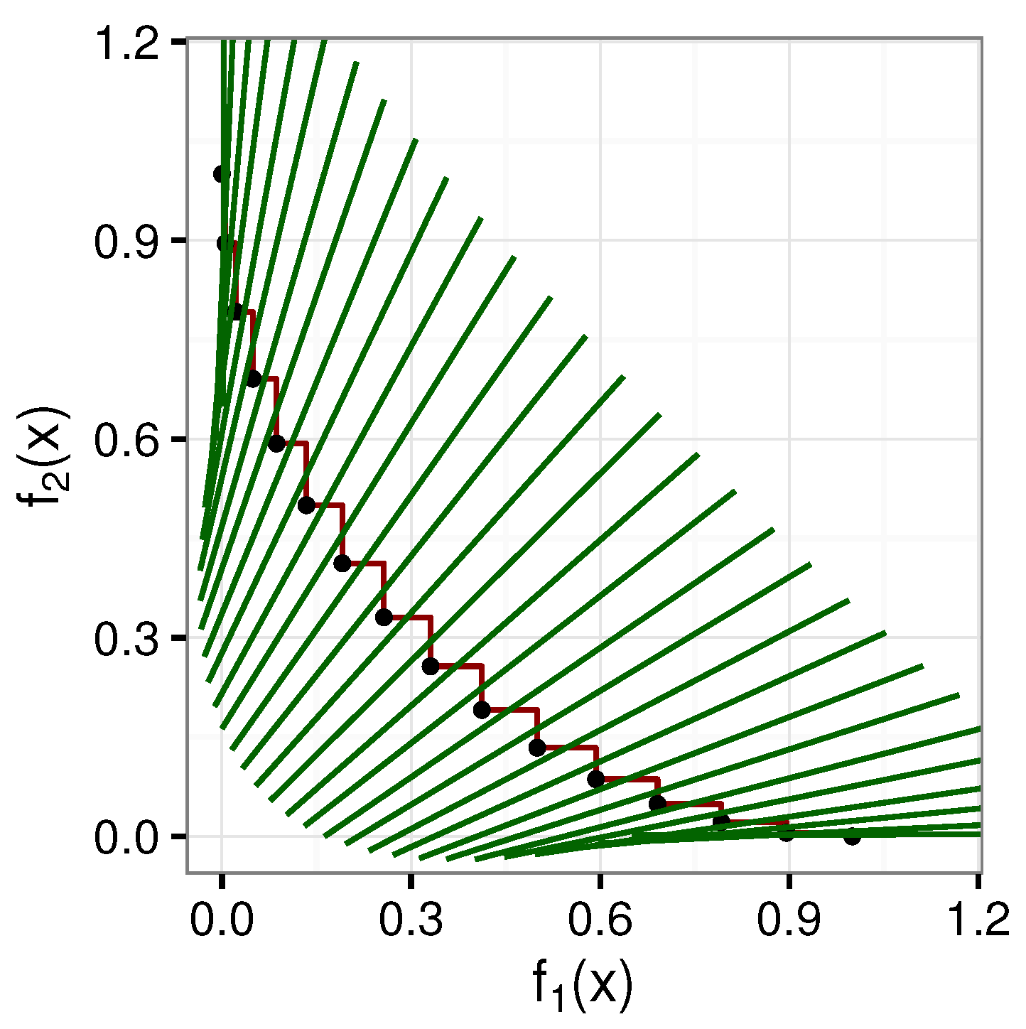
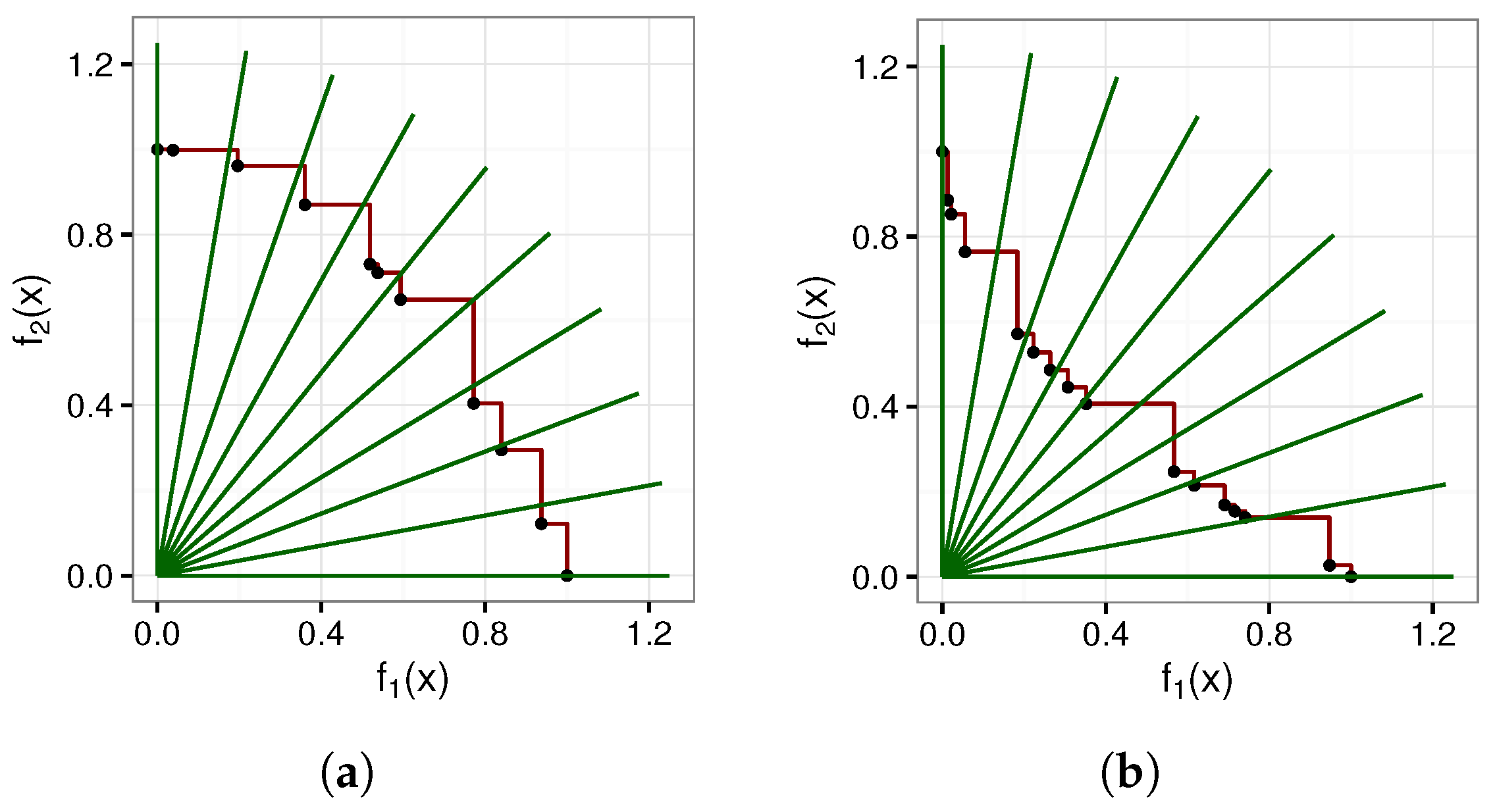
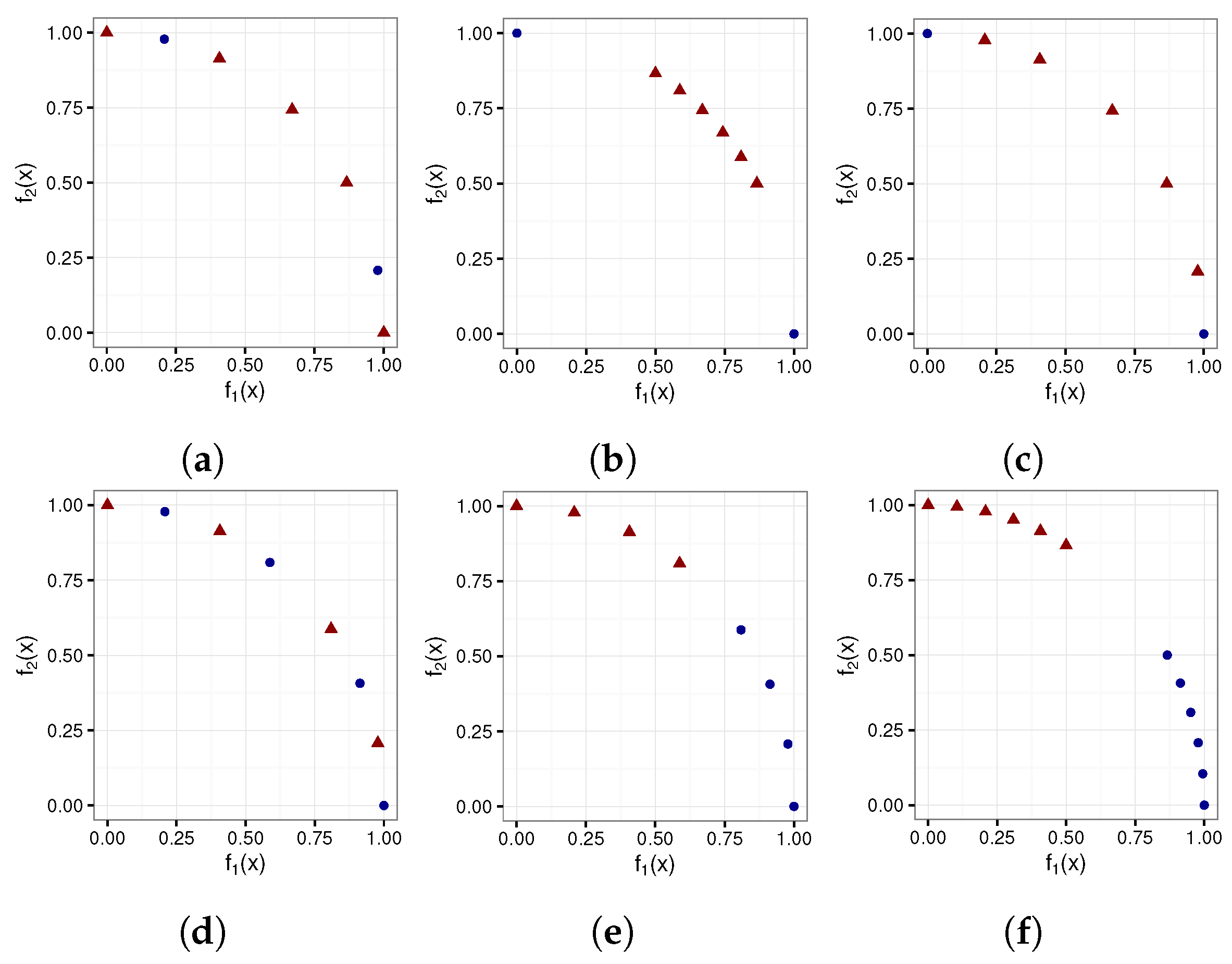
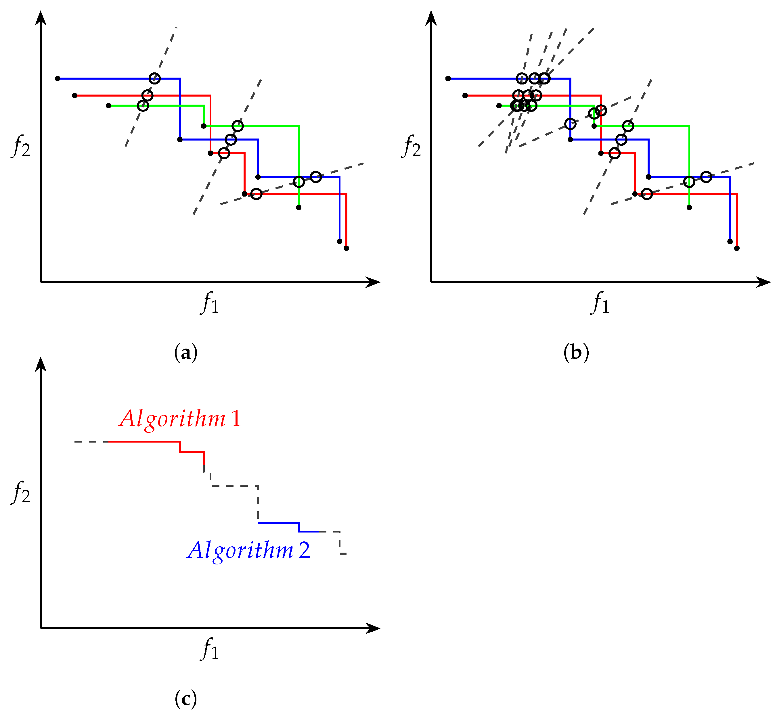
For stochastic algorithms, variations in the performance over multiple runs (also referred to as samples) are expected. Fonseca and Fleming [1] described a procedure to generate an attainment surface that represents a given algorithm’s performance over multiple independent runs. The attainment surface for multiple independent runs is computed by first determining the attainment surface for each run’s approximated POF. Next, a number of random imaginary lines is chosen, pointing in the direction of improvement for all the objectives. For each line, the points of intersection with each of the lines and the attainment surfaces are calculated. Figure 2a,b depict three attainment surfaces with intersection lines and intersection points.

Figure 2. Attainment surfaces. (a) Example attainment surfaces with intersection lines. (b) Example attainment surfaces with unequally spread intersection lines. (c) Grand attainment surface.

For each line, the intersection points can be seen as a sample distribution that is uni-dimensional and can thus be strictly ordered. By calculating the median for each of the sample distributions, the objective vectors that are likely to be attained in exactly $50\%$ of the runs can be identified. The envelope formed by the median points is known as the $50\%$ grand attainment surface. Similar to how the median is used to construct the $50\%$ grand attainment surface, the lower and upper quantiles (25th and 75th percentiles) are used to construct the $25\%$ and $75\%$ grand attainment surfaces.

The sample distribution approach can also be used to compare performance between algorithms. In order to compare two algorithms, two sample distributions—one for each of the algorithms—are calculated per intersection line. Standard non-parametric statistical test procedures can then be used to determine if there is a statistically significant difference between the two sample distributions. Using the statistical test results, a combined grand attainment surface, as depicted in Figure 2c, can be constructed, showing the regions where each of the algorithms outperforms the other. Fonseca and Fleming [1] suggested that suitable test procedures include the median test, its extensions to other quantiles, and tests of the Kolmogorov–Smirnov type [9].

Knowles and Corne [8] extended the work carried out by Fonseca and Fleming and used attainment surfaces to quantify the performance of their Pareto archives evolution strategy (PAES) algorithm. Knowles and Corne identified four variables in the approach proposed by Fonseca and Fleming, namely:

• How many comparison lines should be used;
• Where the comparison lines should go;
• Which statistical test should be used to compare the univariate distribution;
• In what form should the results be presented.

From their empirical analysis, Knowles and Corne found that at least 1000 lines should be used. In order to generate the intersection lines, the minimum and maximum values for each objective over the non-dominated solutions were found. The objective values were then normalized according to the minimum and maximum values into the range $[0,1]$. Intersection lines were then generated as equally spread lines from the origin rotated from $(0,1)$ to $(1,0)$, effectively rotating 90°, covering the complete approximated POF.

For M-dimensional problems, where the number of objectives is $M>2$, Knowles and Corne suggested using a grid-based approach where points are spread equally on the M, $(M-1)$-dimensional hyperplanes. Each hyperplane corresponds to an objective value fixed at the value $1.0$. The intersection lines are drawn from the origin to these equally distributed points. In the case of 3-dimensional problems, a $6\times 6$ grid would result in 108 ($3\times 6\times 6$) points and, thus, 108 intersection lines. Similarly, using a $16\times 16$ grid on a 3-dimensional problem would result in 768 intersection lines, and so forth.

For statistical significance testing, Knowles and Corne used the Mann–Whitney U test [9] with a significance level of $\alpha =0.05$.

Finally, Knowles and Corne found that a convenient way to report the comparison results was to use simple value pairs $[a,b]$, hereafter referred to as the Knowles-Corne measure (KC), where a gives the percentage of space for which algorithm A was found to be statistically superior to algorithm B, and b gives the percentage where algorithm B was found to be statistically superior to algorithm A. It can be noted that $100-(a+b)$ gives the percentage where neither algorithm was found to be statistically superior to the other.

Knowles and Corne [8] generalized the definition of the comparison to compare more than two algorithms. For K algorithms, the above comparison is carried out for all $\left(\genfrac{}{}{0pt}{}{K}{2}\right)$ algorithm pairs. For each algorithm, k, two percentages are reported: $a_k$, which is the region where algorithm k was not worse than any other algorithm, and $b_k$, which is the region where algorithm k performed better than all the other $(K-1)$ algorithms. Note that $a_k\ge b_k$ because the region described by $b_k$ is contained in the region described by $a_k$.

Knowles and Corne [10] found that visualization of attainment surfaces in three dimensions is difficult due to the intersection lines not being evenly spread. As an alternative, Knowles presented an algorithm inspired by the work conducted by Smith et al. [11] to visually draw summary attainment surfaces using axis-aligned lines. The algorithm was found to be particularly well suited for drawing 3-dimensional attainment surfaces.

Fonseca et al. [12] continued work on attainment surfaces by introducing the empirical attainment function (EAF). The EAF is a mean-like, first-order moment measure of the solutions found by a multi-objective optimiser. The EAF allows for intuitive visual comparisons between bi-objective optimization algorithms by plotting the solution probabilities as a heat map [13]. Fonseca et al. [14] studied the use of the second-order EAF, which allows for the pairwise relationship between random Pareto-set approximations to be studied.

It should be noted that calculation of the EAF for three or more dimensions is not trivial [15]. Efficient algorithms to calculate the EAF for two and three dimensions have been proposed in [15]. Tušar and Filipič [16] developed approaches to visualize the EAFs in two and three dimensions.

4. Regarding 2-Dimensional Attainment Surfaces

The attainment surface calculation approach developed by Fonseca and Fleming [1] did not describe in detail how the intersection lines should be generated. Instead, it was only stated that a random number of intersection lines, each pointing in the direction of improvement for all the objectives, should be used. This approach worked well to construct a visualization of the attainment surface.

When Knowles and Corne [8] extended the intersection line approach to develop a quantitative comparison measure, they needed the lines to be equally distributed. If the lines were not equally distributed, as depicted in Figure 2b, certain regions of the attainment surface would contribute more than others, leading to misleading results.

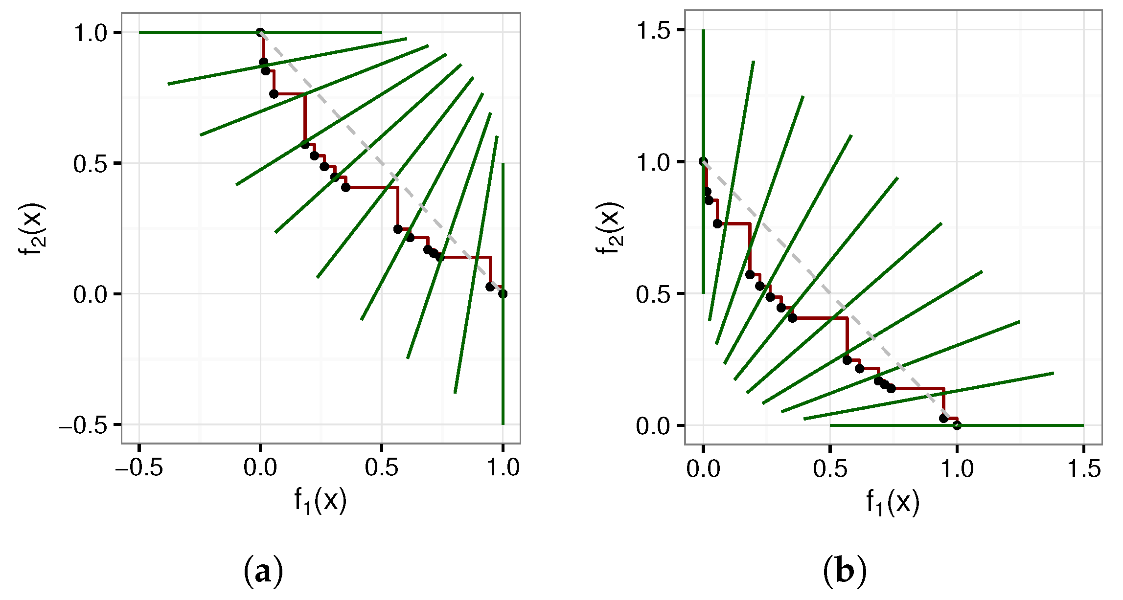
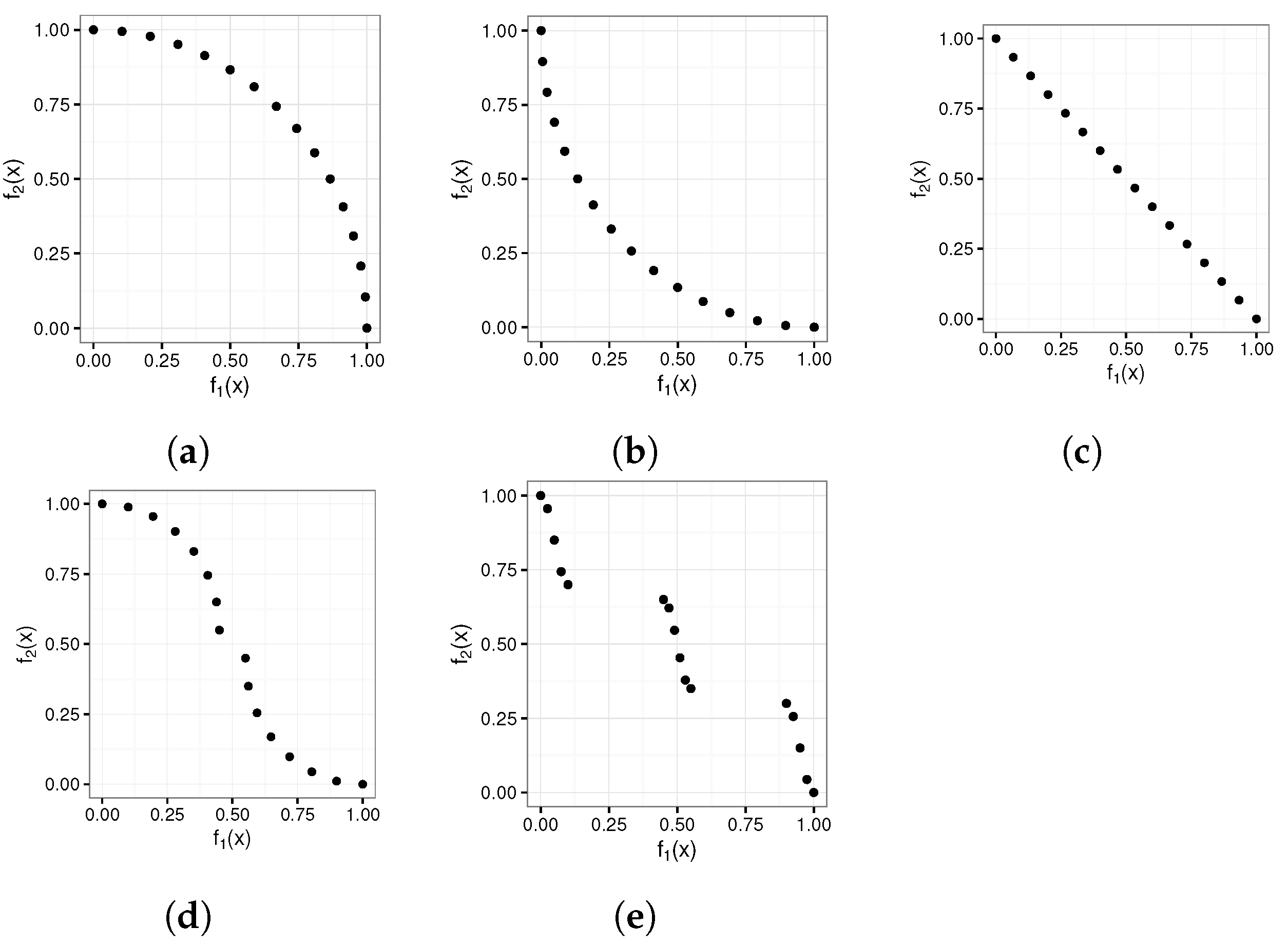
Figure 3 depicts two example attainment surfaces with rotation-based intersection lines. Figure 3a depicts a concave attainment surface. Visually, the rotation-based intersection lines look to be equally distributed. Figure 3b, however, depicts a convex attainment surface. Visually, the length of the attainment surface between the intersection lines is larger in the regions closer to the objective axis than in the middle regions. Clearly, the rotation-based intersection lines are not equally spaced for convex-shaped fronts when comparing the length of the attainment surface represented by each intersection line.

Figure 3. Attainment surfaces with rotation-based intersection lines. (a) Concave POF. (b) Convex POF.

In order to address the unequal spacing of the rotation-based intersection lines, a new approach to placing the intersection lines is proposed in this paper. To compensate for the shape of the front, the intersection lines can be generated either inwardly or outwardly positioned on a line, running from the extreme values of the attainment surface, based on the shape of the attainment surfaces being compared. 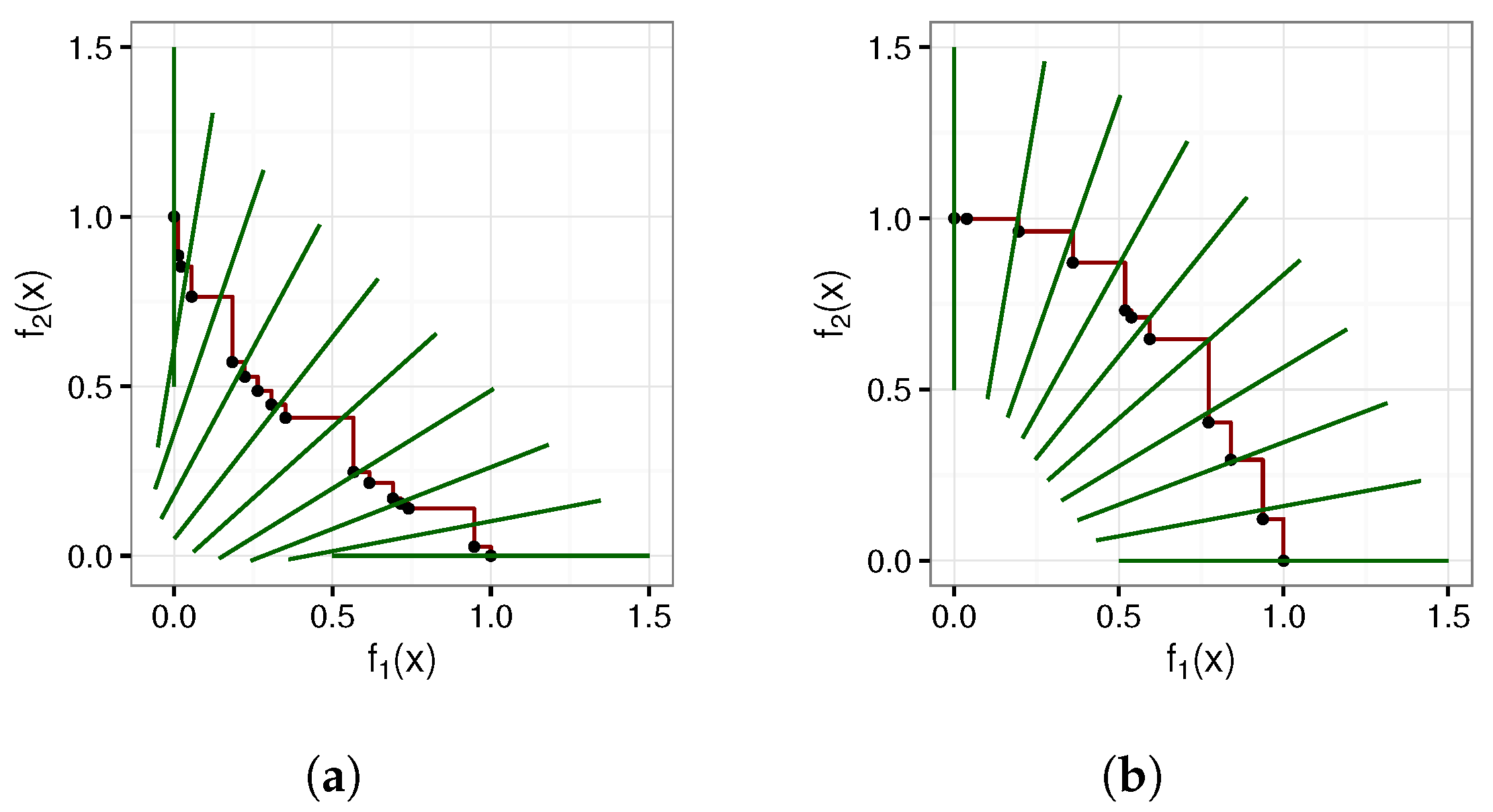Figure 4 depicts the inward and outward intersection line approaches for a convex shaped front. The regions are clearly more equally spread for the inward intersection line approach.

Figure 4. Attainment surfaces with outward/inward intersection lines. (a) Inward. (b) Outward.

However, the direction of the intersection lines is less desirable for comparison purposes. At the edges, the intersection lines are parallel with the opposite objective’s axis. Intuitively, it is more desirable that the intersection lines should be parallel to the closest objective’s axis. Another disadvantage of the inward and outward approaches is that the approach to be selected depends on the shape of the front, which is typically unknown. For attainment surfaces that are not fully convex or concave, neither approach is suitable.

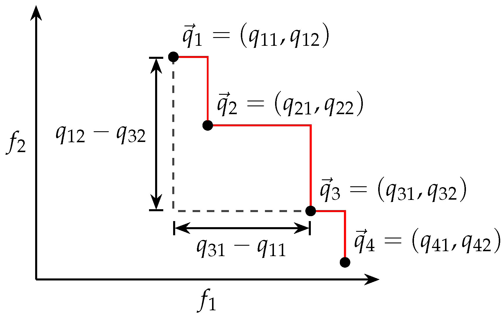
An alternative approach, referred to as attainment-surface-shaped intersection lines (ASSIL) in this paper, is to generate the intersection lines along the shape of the attainment surface. In order to equally spread the intersection lines, the Manhattan distance is used to calculate equal spacings for the intersection lines along the attainment surface. Figure 5 depicts the Manhattan distance calculation between two points on the approximated POF, which is ${\overrightarrow{q}}_3$ and ${\overrightarrow{q}}_1$ in this case. ASSIL can be generated using Algorithm 1.

Algorithm 1 Attainment-surface-shaped intersection line (ASSIL) generation.

1: Input: The optimal POF, $Q=\{\overrightarrow{q_i}:i\in \{1,\dots ,I\}\}$ with I solutions and $\overrightarrow{q_i}=(q_{i1},q_{i2})$   2: Output: An attainment surface   3: Sort Q in ascending order by $q_{i1}$   4: $i\leftarrow 1$   5: Let N be the desired number of intersection lines   6: for $i_n\leftarrow 1,\dots ,N$ do   7:    $d\leftarrow (i_n-1)\times \frac{(q_{I1}-q_{11})+(q_{12}-q_{I2})}{N-1}$   8:    while $d<(q_{i1}-q_{11})+(q_{12}-q_{i2})$ do   9:      $i\leftarrow i+1$ 10:    end while 11:    if $d=(q_{i1}-q_{11})+(q_{12}-q_{i2})$ then 12:      $\overrightarrow{\widehat{q}}\leftarrow {\overrightarrow{q}}_i$ 13:    else if $d\le (q_{(i+1)1}-q_{11})+(q_{12}-q_{i2})$ then 14:      $\overrightarrow{\widehat{q}}\leftarrow (q_{11}+(d-(q_{12}-q_{i2})),q_{i2})$ 15:    else 16:      $\overrightarrow{\widehat{q}}\leftarrow (q_{(i+1)1},q_{12}-(d-(q_{(i+1)1}-q_{11})))$ 17:    end if 18:    $\theta \leftarrow \frac{i_N-1}{N-1}\times \frac{\pi }{2}$ 19:    $From\leftarrow ({\widehat{q}}_1-sin\theta ,{\widehat{q}}_2-cos\theta )$ 20:    $To\leftarrow ({\widehat{q}}_1+sin\theta ,{\widehat{q}}_2+cos\theta )$ 20:    // Finally, draw the generated intersection line 21:    drawIntersectionLine($From$, $To$) 22: end for

Figure 5. Attainment surface with Manhattan distance calculations.

Intersection lines are spaced equally along the attainment surface. The intersection lines are rotated incrementally such that the intersection lines at the ends of the attainment surface are parallel to the objective axis.

Figure 6 depicts the attainment-surface-shaped intersection line approach. The generation of the intersection lines along the shape of the attainment surface allows for an equal spacing of the intersection lines independent of the shape of the front. For all shapes that the attainment surface can assume, whether convex, concave, or mixed, the intersection lines are equally spread out.

Figure 6. Attainment surfaces with unbiased ASSIL. (a) Convex POF. (b) Concave POF.

The KC measure is calculated as shown in Algorithm 2.

Algorithm 2 Algorithm for the calculation of the KC measure.

1: Input: Intersection lines for algorithms A and B to be compared   2: Output: The KC measure   3: Let $total=0$   4: Let $win{s}_A=0$   5: Let $win{s}_B=0$   6: for each intersection line l do   7:    Let O be the strict ordering of the intersection points for algorithms A and B on intersection line l   8:    Let $O_A\subset O$ be the ordering of the intersection points for algorithm A on intersection line l   9:    Let $O_B\subset O$ be the ordering of the intersection points for algorithm B on intersection line l 10:    if $O_A$ is statistically significantly less than $O_B$ then 11:      $win{s}_A=win{s}_A+1$ 12:    else if $O_B$ is statistically significantly less than $O_A$ then 13:      $win{s}_B=win{s}_B+1$ 14:    end if 15:    $total=total+1$ 16: end for 17: Return $[\frac{100win{s}_A}{total},\frac{100win{s}_B}{total}]$

An evaluation of the rotation-based and random intersection line approaches is presented using six artificially generated POF test cases based on those used by Knowles and Corne [8]. Figure 7 depicts the six artificially generated POF test cases. Each of these artificially generated POF test cases was tested using six pof shape geometries, namely concave, convex, linear, mixed, and disconnected geometries. Figure 8 depicts the five POF shape geometries.

Figure 7. Test case Pareto-optimal fronts. Dots represent algorithm A, and triangles represent algorithm B. (a) Case 1. (b) Case 2. (c) Case 3. (d) Case 4. (e) Case 5. (f) Case 6.

Figure 8. Test case Pareto-optimal front geometries. (a) Concave. (b) Convex. (c) Linear. (d) Mixed. (e) Disconnected.

Table 1 summarises the true KC, the KC with rotation-based and random intersection lines, and the KC with ASSIL results. Values in red indicate attainment surfaces obtained that outperformed the control method (i.e., the true KC measure) by more than 5%, while values in blue indicate attainment surfaces that were found that were 5% worse than the control method. For each of the approaches, 1000 intersection lines were used for the calculation.

Table 1. Comparison of the results of KC measure with ASSIL; blue indicates performance of 5% worse than the competing algorithm, and red indicates performance of 5% better than the competing algorithm.

Case	Geometry	True	Intersection Line Generation Approach
			Rotation-Based	Random	ASSIL
Case 1	Concave	(73.27, 26.73)	(71.00, 29.00)	(76.80, 23.20)	(73.20, 26.80)
	Convex	(70.37, 29.63)	(85.10, 14.90)	(85.60, 14.40)	(70.30, 29.70)
	Line	(70.00, 30.00)	(74.60, 25.40)	(79.30, 20.70)	(70.00, 30.00)
	Mixed	(69.67, 30.33)	(73.20, 26.80)	(82.10, 17.90)	(69.80, 30.20)
	Disconnected	(77.50, 22.50)	(82.70, 17.30)	(86.90, 13.10)	(77.50, 22.50)
Case 2	Concave	(50.00, 50.00)	(41.00, 59.00)	(67.60, 32.40)	(50.00, 50.00)
	Convex	(86.60, 13.40)	(83.00, 17.00)	(96.40, 3.60)	(86.60, 13.40)
	Line	(66.67, 33.33)	(59.00, 41.00)	(81.30, 18.70)	(66.60, 33.40)
	Mixed	(66.99, 33.01)	(59.60, 40.40)	(81.60, 18.40)	(66.90, 33.10)
	Disconnected	(60.00, 40.00)	(51.60, 48.40)	(75.80, 24.20)	(60.00, 40.00)
Case 3	Concave	(79.21, 20.79)	(73.80, 26.20)	(92.60, 7.40)	(79.20, 20.80)
	Convex	(97.81, 2.19)	(97.20, 2.80)	( 99.90, 0.10)	(97.80, 2.20)
	Line	(86.67, 13.33)	(83.00, 17.00)	(96.50, 3.50)	(86.60, 13.40)
	Mixed	(88.01, 11.99)	(84.80, 15.20)	(95.60, 4.40)	(87.90, 12.10)
	Disconnected	(90.00, 10.00)	(87.30, 12.70)	(97.60, 2.40)	(90.00, 10.00)
Case 4	Concave	(50.00, 50.00)	(50.00, 50.00)	(49.00, 51.00)	(50.00, 50.00)
	Convex	(50.00, 50.00)	(50.00, 50.00)	(50.60, 49.40)	(50.00, 50.00)
	Line	(50.00, 50.00)	(50.00, 50.00)	(54.00, 46.00)	(50.00, 49.90)
	Mixed	(55.71, 44.29)	(54.30, 45.70)	(50.70, 49.30)	(55.70, 44.30)
	Disconnected	(69.14, 30.86)	(73.00, 27.00)	(77.80, 22.20)	(69.10, 30.90)
Case 5	Concave	(50.00, 50.00)	(50.00, 50.00)	(49.50, 50.50)	(50.00, 50.00)
	Convex	(50.00, 50.00)	(50.00, 50.00)	(50.40, 49.60)	(50.00, 50.00)
	Line	(50.00, 50.00)	(50.00, 50.00)	(49.20, 50.80)	(50.00, 50.00)
	Mixed	(45.56, 54.44)	(45.30, 54.70)	(43.40, 56.60)	(45.60, 54.40)
	Disconnected	(45.43, 54.57)	(45.00, 55.00)	(45.40, 54.60)	(45.40, 54.60)
Case 6	Concave	(50.00, 50.00)	(50.00, 50.00)	(48.00, 52.00)	(50.00, 50.00)
	Convex	(50.00, 50.00)	(50.00, 50.00)	(49.50, 50.50)	(50.00, 50.00)
	Line	(50.00, 50.00)	(50.00, 50.00)	(49.30, 50.70)	(50.00, 50.00)
	Mixed	(42.47, 57.53)	(42.90, 57.10)	(37.70, 62.30)	(42.50, 57.50)
	Disconnected	(45.00, 55.00)	(44.70, 55.30)	(44.10, 55.90)	(45.00, 55.00)

As expected, the ASSIL generation approach produced results much closer to the true KC measure: the closer the POFs being compared are to the true POF, the more accurate the comparison using the ASSIL generation approach becomes.

Table 2 and Table 3 present a comparison of the varying results obtained from using the various intersection line generation approaches. Results comparing the vector evaluated particle swarm optimization (VEPSO) [17], optimized multi-objective particle swarm optimization (OMOPSO) [18], and speed-constrained multi-objective particle swarm optimization (SMPSO) [19] algorithms using the Zitzler-Deb-Thiele (ZDT) [20] and Walking Fish Group (WFG) [21] test sets are presented. The choice of algorithms was arbitrary and only for illustrative purposes. Results were obtained over 30 independent runs. For more details on the algorithms and parameters used, the interested reader is referred to [22]. The characteristics of the problems are summarized in Table 4.

Table 2. Intersection line comparison between VEPSO ($\mathcal{V}$), SMPSO ($\mathcal{S}$), and OMOPSO ($\mathcal{O}$); blue indicates performance of 5% worse than the competing algorithm, and red indicates performance of 5% better than the competing algorithm.

Problem	Intersections	$\mathcal{V}$ vs. $\mathcal{O}$	$\mathcal{V}$ vs. $\mathcal{S}$	$\mathcal{S}$ vs. $\mathcal{O}$
ZDT1	Rotational	(14.9,66.4)	(6.1,80.6)	(79.4,1.1)
	Inward	$(25.6,55.5)$	(13.8, 65.4)	$(70.2,3.9)$
	Outward	$(19.8,62.7)$	$(8.7,75.6)$	$(77.3,1.6)$
	ASSIL	$(22.5,60.1)$	$(11.4,72.2)$	$(72.5,4.3)$
ZDT2	Rotational	$(8.4,64.3)$	$(2.9,73.6)$	$(58.9,3.9)$
	Inward	$(8.0,63.4)$	$(2.0,74.3)$	$(56.3,0.9)$
	Outward	$(10.4,62.7)$	$(4.2,70.5)$	$(60.1,5.7)$
	ASSIL	$(9.0,63.9)$	$(3.4,72.6)$	$(60.0,3.8)$
ZDT3	Rotational	(13.4, 77.9)	$(3.9,90.8)$	(81.4, 7.3)
	Inward	(7.1, 61.6)	(2.1, 83.2)	$(72.4,10.5)$
	Outward	$(16.4,73.2)$	$(4.9,87.7)$	$(78.4,8.7)$
	ASSIL	$(12.5,72.9)$	$(3.2,89.3)$	$(74.8,9.5)$
ZDT4	Rotational	$(0.0,99.9)$	$(0.0,99.9)$	(99.9, 0.0)
	Inward	(0.0, 87.9)	(0.0, 88.1)	(80.9, 0.0)
	Outward	$(0.0,100.0)$	$(0.0,100.0)$	(100.0, 0.0)
	ASSIL	$(0.0,100.0)$	$(0.0,97.7)$	$(93.7,0.0)$
ZDT6	Rotational	(40.1, 13.3)	(15.2, 25.9)	(58.9, 11.1)
	Inward	(64.6, 2.8)	(15.6, 35.3)	(73.3, 0.7)
	Outward	(50.6, 7.8)	(6.1, 52.9)	(64.5, 5.0)
	ASSIL	$(59.4,4.3)$	$(10.9,41.8)$	$(52.3,14.1)$

Table 3. Intersection line comparison between VEPSO ($\mathcal{V}$), SMPSO ($\mathcal{S}$), and OMOPSO ($\mathcal{O}$); blue indicatses performance of 5% worse than the competing algorithm, and red indicates performance of 5% better than the competing algorithm.

Problem	Intersections	$\mathcal{V}$ vs. $\mathcal{O}$	$\mathcal{V}$ vs. $\mathcal{S}$	$\mathcal{S}$ vs. $\mathcal{O}$
WFG1	Rotational	$(0.0,99.9)$	$(0.2,96.9)$	$(28.6,65.8)$
	Inward	$(0.0,100.0)$	$(0.2,97.6)$	(38.4,55.6)
	Outward	$(0.0,99.9)$	$(0.2,97.5)$	$(26.6,68.0)$
	ASSIL	$(0.0,99.9)$	$(0.2,97.5)$	$(27.2,67.2)$
WFG2	Rotational	$(0.0,99.9)$	$(0.0,99.9)$	(0.0,65.5)
	Inward	$(0.0,100.0)$	$(0.0,100.0)$	(0.0,86.6)
	Outward	$(0.0,99.9)$	$(0.0,99.9)$	(0.0,63.9)
	ASSIL	$(0.0,99.9)$	$(0.0,99.9)$	$(0.0,73.1)$
WFG3	Rotational	$(0.0,99.9)$	$(0.0,99.9)$	$(0.0,88.8)$
	Inward	$(0.0,100.0)$	$(0.0,100.0)$	$(0.0,87.3)$
	Outward	$(0.0,99.9)$	$(0.0,99.9)$	$(0.0,89.2)$
	ASSIL	$(0.0,99.9)$	$(0.0,99.9)$	$(0.0,88.8)$
WFG4	Rotational	$(0.0,99.9)$	$(0.0,99.9)$	$(99.9,0.0)$
	Inward	$(0.0,100.0)$	$(0.0,100.0)$	$(100.0,0.0)$
	Outward	$(0.0,99.9)$	$(0.0,99.9)$	$(99.9,0.0)$
	ASSIL	$(0.0,99.9)$	$(0.0,99.9)$	$(99.9,0.0)$
WFG5	Rotational	$(16.9,20.0)$	$(0.1,62.7)$	$(52.4,2.0)$
	Inward	(10.1,21.0)	$(0.2,59.8)$	(39.9,0.5)
	Outward	$(18.6,23.4)$	$(0.2,64.4)$	$(55.0,2.9)$
	ASSIL	$(16.2,19.1)$	$(0.2,61.1)$	$(50.3,1.7)$
WFG6	Rotational	$(25.6,13.5)$	$(0.0,99.9)$	$(99.9,0.0)$
	Inward	(9.9,13.5)	$(0.0,100.0)$	$(100.0,0.0)$
	Outward	(29.6,13.7)	$(0.0,99.9)$	$(99.9,0.0)$
	ASSIL	$(23.3,13.7)$	$(0.0,99.9)$	$(99.9,0.0)$
WFG7	Rotational	$(0.0,99.9)$	$(0.0,99.9)$	$(0.0,92.7)$
	Inward	$(0.0,100.0)$	$(0.0,100.0)$	$(0.0,95.4)$
	Outward	$(0.0,99.9)$	$(0.0,99.9)$	$(0.0,92.6)$
	ASSIL	$(0.0,99.9)$	$(0.0,99.9)$	$(0.0,93.2)$
WFG8	Rotational	$(0.0,99.9)$	$(0.0,99.9)$	$(0.0,94.6)$
	Inward	$(0.0,100.0)$	$(0.0,100.0)$	$(0.0,95.8)$
	Outward	$(0.0,99.9)$	$(0.0,99.9)$	$(0.0,94.4)$
	ASSIL	$(0.0,99.9)$	$(0.0,99.9)$	$(0.0,95.1)$
WFG9	Rotational	$(8.0,30.3)$	$(0.0,99.9)$	$(99.9,0.0)$
	Inward	(2.6,41.1)	$(0.0,100.0)$	$(100.0,0.0)$
	Outward	$(8.8,27.9)$	$(0.0,99.9)$	$(99.9,0.0)$
	ASSIL	$(7.1,31.5)$	$(0.0,99.9)$	$(99.9,0.0)$

Table 4. Properties of the ZDT and WFG problems.

Name	Separability	Modality	Geometry
ZDT1	Separable	Unimodal	Convex
ZDT2	Separable	Unimodal	Concave
ZDT3	Separable	Unimodal/multimodal	Disconnected
ZDT4	Separable	Unimodal/multimodal	Convex
ZDT6	Separable	Multimodal	Concave
WFG1	Separable	Unimodal	Convex, mixed
WFG2	Non-separable	Unimodal/multimodal	Convex, disconnected
WFG3	Non-separable	Unimodal	Linear, degenerate
WFG4	Separable	Multimodal	Concave
WFG5	Separable	Multimodal	Concave
WFG6	Non-separable	Unimodal	Concave
WFG7	Separable	Unimodal	Concave
WFG8	Non-separable	Unimodal	Concave
WFG9	Non-separable	Multimodal, deceptive	Concave

Variations in the results between the different intersection line generation approaches can be seen. ZDT1, ZDT3, ZDT4, and ZDT6 all show variations in the results greater than $5\%$ for each of the comparisons. WFG1, WFG2, WFG5, WFG6, and WFG9 all show variations in the results greater than $5\%$ for at least one of the comparisons. The variations are indicative of the bias towards certain attainment surface shapes shown by the various intersection line generation approaches.

5. Weighted 2-Dimensional Attainment-Surface-Shaped Intersection Lines

As an alternative to the equally spread intersection lines used by ASSIL, intersection lines can be generated along the shape of the POF, with at least one intersection line per attainment surface line segment. Because the attainment surface segments are not all of equal lengths, a weight is associated with each intersection line to balance the KC measure result. The weighted attainment-surface-shaped intersection lines (WASSIL) generation algorithm is given in Algorithm 3.

Figure 9 depicts a convex POF with WASSIL-generated intersection lines. The figure clearly shows that the intersection lines are positioned along the attainment surface, and due to the positioning, the lines are angled slightly differently from the intersection lines in Figure 3b. The WASSIL algorithm should, for the test cases, result in a weighted KC measure result that matches the true KC measure result.

Figure 9. Convex POF and attainment surface with WASSILs.

Note that the weighted KC measure is calculated as shown in Algorithm 4.

Table 5 summarises the true KC measure, the KC measure with rotation-based and random intersection lines, the KC measure with ASSIL, and the KC measure with WASSIL results. For each of the approaches, 1000 intersection lines were used for the calculation.

Algorithm 3 Weighted attainment-surface-shaped intersection line (WASSIL) generation.

1: Input: The optimal POF, $Q=\{\overrightarrow{q_i}:i\in \{1,\dots ,I\}\}$ with I solutions and $\overrightarrow{q_i}=(q_{i1},q_{i2})$   2: Output: An attainment surface   3: for each attainment line segment $s_l$ do   4:    Let $w_l=length(s_l)$   5:    Let $\mathbf{c}$ be the center of $s_l$   6:    Let $\theta =\frac{\pi (c_1+(max(q_{i2}-c_2))}{2d}$, for $i=1,\dots ,I$   7:    Let $\mathbf{p}=(sin\theta ,cos\theta )$   8:    //Draw the generated intersection line   9:    drawIntersectionLineWithWeight(from=$\mathbf{c}-\mathbf{p}$,to=$\mathbf{c}+\mathbf{p}$,weight=$w_l$) 10: end for

Table 5. Comparison of the results of the KC measure with WASSIL; blue indicates performance of 5% worse than the competing algorithm, and red indicates performance of 5% better than the competing algorithm.

Case	Geometry	True	Intersection Line Generation Approach
			Rotation-Based	Random	ASSIL	WASSIL
Case 1	Concave	(73.27, 26.73)	(71.00, 29.00)	(79.90, 20.10)	(73.20, 26.80)	(73.27, 26.73)
	Convex	(70.37, 29.63)	(85.10, 14.90)	(87.40, 12.60)	(70.30, 29.70)	(70.37, 29.63)
	Line	(70.00, 30.00)	(74.60, 25.40)	(78.80, 21.20)	(70.00, 30.00)	(70.00, 30.00)
	Mixed	(69.67, 30.33)	(73.20, 26.80)	(78.30, 21.70)	(69.80, 30.20)	(69.67, 30.33)
	Disconnected	(77.50, 22.50)	(82.70, 17.30)	(87.60, 12.40)	(77.50, 22.50)	(77.50, 22.50)
Case 2	Concave	(50.00, 50.00)	(41.00, 59.00)	(67.00, 33.00)	(50.00, 50.00)	(50.00, 50.00)
	Convex	(86.60, 13.40)	(83.00, 17.00)	(97.20, 2.80)	(86.60, 13.40)	(86.60, 13.40)
	Line	(66.67, 33.33)	(59.00, 41.00)	(85.60, 14.40)	(66.60, 33.40)	(66.67, 33.33)
	Mixed	(66.99, 33.01)	(59.60, 40.40)	(82.10, 17.90)	(66.90, 33.10)	(66.99, 33.01)
	Disconnected	(60.00, 40.00)	(51.60, 48.40)	(77.40, 22.60)	(60.00, 40.00)	(60.00, 40.00)
Case 3	Concave	(79.21, 20.79)	(73.80, 26.20)	(93.20, 6.80)	(79.20, 20.80)	(79.21, 20.79)
	Convex	(97.81, 2.19)	(97.20, 2.80)	(100.00, 0.00)	(97.80, 2.20)	(97.81, 2.19)
	Line	(86.67, 13.33)	(83.00, 17.00)	(96.60, 3.40)	(86.60, 13.40)	(86.67, 13.33)
	Mixed	(88.01, 11.99)	(84.80, 15.20)	(95.70, 4.30)	(87.90, 12.10)	(88.01, 11.99)
	Disconnected	(90.00, 10.00)	(87.30, 12.70)	(97.50, 2.50)	(90.00, 10.00)	(90.00, 10.00)
Case 4	Concave	(50.00, 50.00)	(50.00, 50.00)	(49.40, 50.60)	(50.00, 50.00)	(50.00, 50.00)
	Convex	(50.00, 50.00)	(50.00, 50.00)	(48.70, 51.30)	(50.00, 50.00)	(50.00, 50.00)
	Line	(50.00, 50.00)	(50.00, 50.00)	(52.30, 47.70)	(50.00, 49.90)	(50.00, 50.00)
	Mixed	(55.71, 44.29)	(54.30, 45.70)	(51.00, 49.00)	(55.70, 44.30)	(55.71, 44.29)
	Disconnected	(69.14, 30.86)	(73.00, 27.00)	(76.70, 23.30)	(69.10, 30.90)	(69.14, 30.86)
Case 5	Concave	(50.00, 50.00)	(50.00, 50.00)	(48.90, 51.10)	(50.00, 50.00)	(50.00, 50.00)
	Convex	(50.00, 50.00)	(50.00, 50.00)	(47.80, 52.20)	(50.00, 50.00)	(50.00, 50.00)
	Line	(50.00, 50.00)	(50.00, 50.00)	(51.00, 49.00)	(50.00, 50.00)	(50.00, 50.00)
	Mixed	(45.56, 54.44)	(45.30, 54.70)	(43.40, 56.60)	(45.60, 54.40)	(45.56, 54.44)
	Disconnected	(45.43, 54.57)	(45.00, 55.00)	(40.60, 59.40)	(45.40, 54.60)	(45.43, 54.57)
Case 6	Concave	(50.00, 50.00)	(50.00, 50.00)	(51.70, 48.30)	(50.00, 50.00)	(50.00, 50.00)
	Convex	(50.00, 50.00)	(50.00, 50.00)	(48.60, 51.40)	(50.00, 50.00)	(50.00, 50.00)
	Line	(50.00, 50.00)	(50.00, 50.00)	(51.70, 48.30)	(50.00, 50.00)	(50.00, 50.00)
	Mixed	(42.47, 57.53)	(42.90, 57.10)	(38.50, 61.50)	(42.50, 57.50)	(42.47, 57.53)
	Disconnected	(45.00, 55.00)	(44.70, 55.30)	(42.60, 57.40)	(45.00, 55.00)	(45.00, 55.00)

For POF test cases 1 through 3, only 2 of the 15 measurements using the random intersection line generation approach had a deviation from the true KC of less than $5\%$. Overall, $50\%$ of the measurements using the random intersection line generation approach had a deviation greater than $5\%$. This confirms that the random intersection line generation approach is not well suited for the KC calculation.

The rotation-based intersection line generation approach presented by Knowles and Corne fared better than the random intersection line generation approach. Only 7 of the 30 measurements using the rotation-based intersection line generation approach had a deviation greater than $5\%$. Case 1 with a convex POF fared worse with a deviation of almost $15\%$ for both algorithms. Four of the five case 2 measurements using the rotation-based intersection line generation approach had a deviation greater than $5\%$. For the remaining case 2 measurement, a deviation of at least $3\%$ is noted. The results indicate the rotation-based intersection line generation approach outperformed the random intersection line generation approach with respect to accuracy. However, the results also indicate that the rotation-based intersection line generation approach is not well suited for the KC calculation and that the results vary based on the POF shape and the spread of the solutions.

As expected, the WASSIL generation approach produced results much closer to the true KC: the closer the approximated POFs being compared are to the true POF, the more accurate the comparison using the WASSIL generation approach becomes.

Algorithm 4 Weighted KC measure algorithm

1: Input: Intersection lines for algorithms A and B to be compared   2: Output: The weighted KC measure   3: Let $w_{total}=0$   4: Let $win{s}_A=0$   5: Let $win{s}_B=0$   6: for each intersection line l do   7:    Let $w_l$ be the weight associated with l   8:    Let O be the strict ordering of the intersection points for algorithms A and B on intersection line l   9:    Let $O_A\subset O$ be the ordering of the intersection points for algorithm A on intersection line l 10:    Let $O_B\subset O$ be the ordering of the intersection points for algorithm B on intersection line l 11:    if $O_A$ is statistically significantly less than $O_B$ then 12:      $win{s}_A=win{s}_A+w_l$ 13:    else if $O_B$ is statistically significantly less than $O_A$ then 14:      $win{s}_B=win{s}_B+w_l$ 15:    end if 16:    $w_{total}=w_{total}+w_l$ 17: end for 18: Return $[\frac{100win{s}_A}{w_{total}},\frac{100win{s}_B}{w_{total}}]$

6. $\mathit{M}$-Dimensional Attainment Surfaces

For M-dimensional problems, Knowles and Corne [8] recommended that a grid-based intersection line generation approach, as explained in Section 3, be used. Similar to the rotational approach for 2-dimensional problems, the grid-based approach would lead to unbalanced intersection lines when measuring irregularly shaped POFs. Figure 10 shows an example of an irregularly shaped 3-dimensional attainment surface.

Figure 10. 3-dimensional attainment surface.

Section 6.1 discusses the challenges that need to be addressed in order to generate intersection lines for M-dimensional attainment surfaces. Section 6.2 and Section 6.3 introduce two algorithms to generate M-dimensional attainment surface intersection lines. The first uses a naive (and computationally expensive) approach that produces all possible intersection lines. The second is computationally more efficient, considering a minimal set of intersection lines. Section 6.4 presents a stability analysis of the two proposed algorithms to show that the computationally efficient approach performs similarly to the naive approach with respect to comparison accuracy.

6.1. Generalizing Attainment Surface Intersection Line Generation to M Dimensions

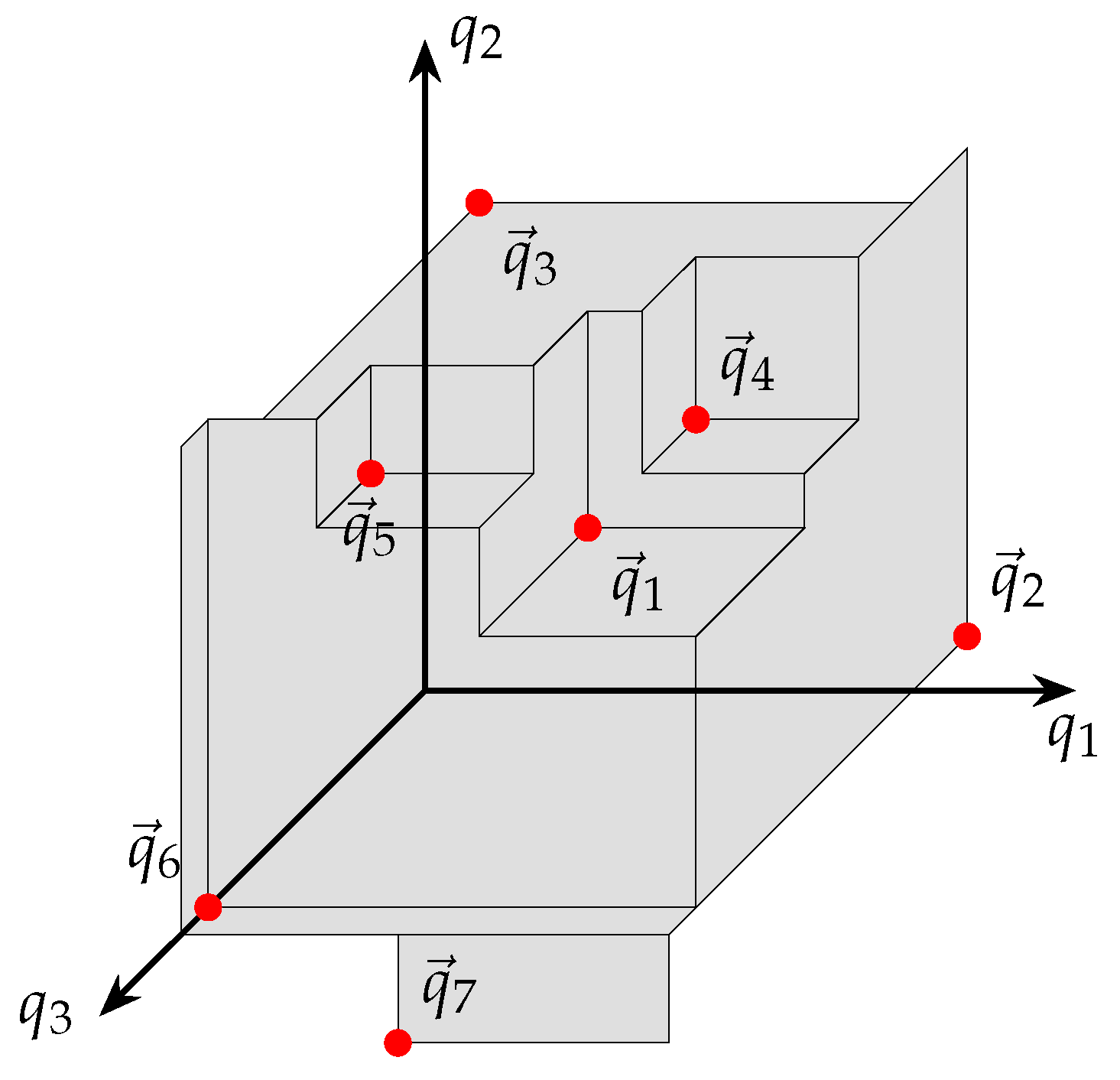
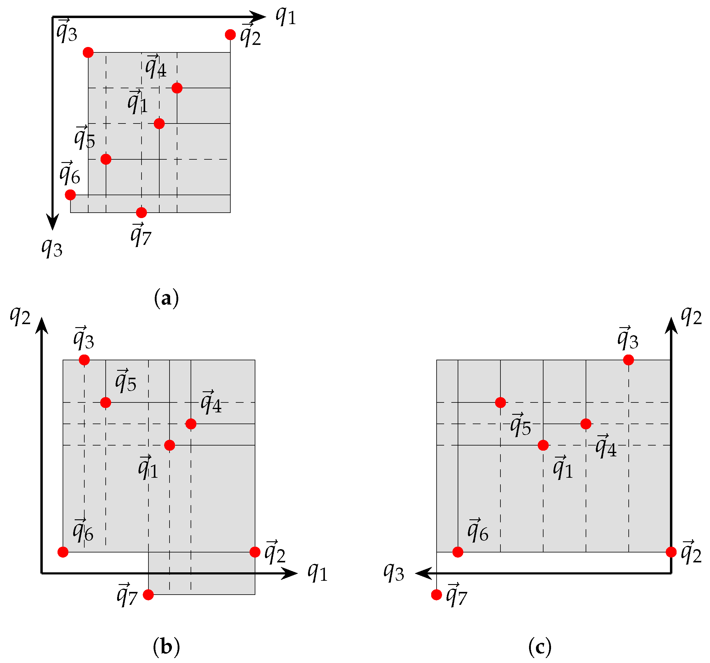
For 2-dimensional problems, the ASSIL approach generates equally spread intersection lines. Intuitively, generalization of the assil approach for M dimensions requires the calculation of equally spread points over the M-dimensional attainment surface.

The calculation of equally spread points requires that the surface is divided into equally sized $M-1$-dimensional hypercubes. For the 3-dimensional case, this would require dividing the attainment surface into equally sized squares. The intersection vectors would be positioned from the middle of each square. The length of the edges would need to be set to the greatest common divider of the lengths of the edges that make up the attainment surface. Even for simple cases, this would lead to an excessive number of squares. The more squares, the higher the computational cost of the measure.

In order to lower the computational cost of the measure, the number of squares needs to be reduced. Because the square edge lengths are based on the greatest common divider, there is no way to reduce the number of squares as long as the squares must be equal in size. If the square sizes differ, the measure will be biased to areas with smaller squares. Areas with smaller squares will carry more weight in the calculation because there will be more of them.

In contrast to the ASSIL approach, the WASSIL approach does not require the intersection lines to be equally spread; instead, only a weight factor must be known for each intersection line. For the 3-dimensional case, the weight factor for each intersection line is calculated as the area of the squares that make up the attainment surface. The weight factor for each intersection line is calculated as the area of the square by multiplying the edge lengths. The weight factor also allows use of rectangles in the 3-dimensional case (hyper-rectangles in the M-dimensional case) instead of equally sized squares.

6.2. Porcupine Measure (Naive Implementation)

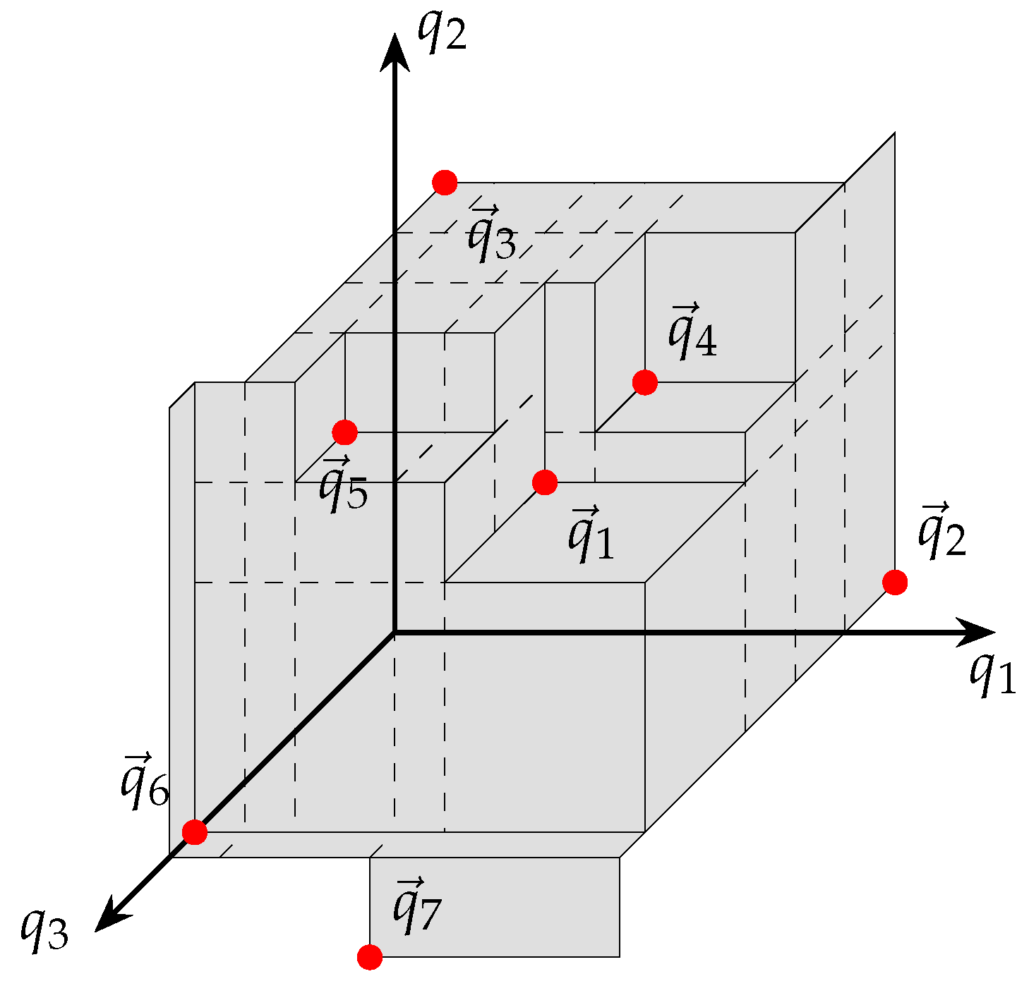
This section presents the naive implementation for the n-dimensional attainment-surface-based quantitative measurement named the porcupine measure. The naive implementation uses each of the n-dimensional values from each Pareto-optimal point to subdivide the attainment surface in each of the dimensions. Figure 11 depicts an example of the subdivision approach for each of the three dimensions, considering all intersection lines. 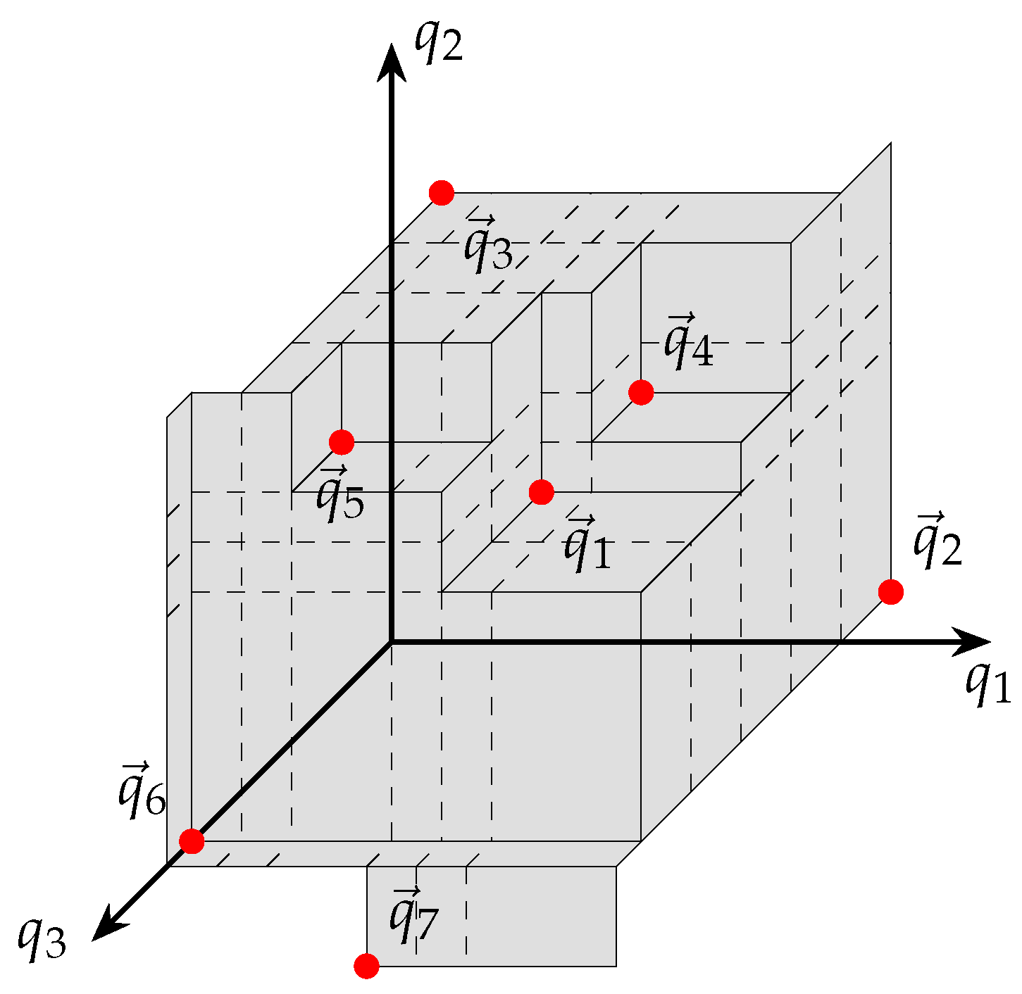Figure 12 depicts the attainment surface, in 3-dimensional space, with the subdivisions visible.

Figure 11. Top, front, and side view of attainment surface with naive subdivisions. (a) Top. (b) Front. (c) Side.

Figure 12. A 3-dimensional attainment surface with naive subdivisions.

In addition to the calculation of the hyper-rectangles, the center point and intersection vector need to be calculated. The naive implementation of the porcupine measure is summarized in Algorithm 5. For a more detailed algorithm listing, please refer to Appendix A.

Using the intersection lines generated by the above algorithm, two algorithms can now be compared using a nonparametric statistical test, such as the Mann–Whitney U test [9]. The porcupine measure is defined, similar to the weighted KC measure, as the weighted sum of the intersection lines where a statistically significant difference exists over the sum of all the weights (i.e., the percentage of the surface area of the attainment surface, as determined by the weights, where one algorithm statistically performs superior to another).

Algorithm 5 Porcupine measure (naive implementation).

1: Input: The found POF   2: Output: The porcupine attainment surface   3: for each of the objective space basis vectors, $m_c$, do   4:    Project the attainment surface parallel to the basis vector, $m_c$, onto the orthogonal $(M-1)$-dimensional subspace   5:    Subdivide the projected attainment surface, in each dimension at every Pareto-optimal point’s dimensional value, into hyper-rectangles   6:    for each hyper-rectangle do   7:      Let $\overrightarrow{c}$ be the center point of the hyper-rectangle   8:      Let w be the weight of the hyper-rectangle, equal to the product of the hyper-rectangle’s edge lengths   9:      for each dimension in objective space $m\in \{1,\dots ,M\}$ do 10:          Let ${min}_m$ be the smallest of the mth-dimensional values of all the Pareto-optimal points where at least one other dimensional value is less than or equal to that of the corresponding center vector’s dimensional value 11:         Let ${max}_m$ be the largest of the mth-dimensional values of all the Pareto-optimal points 12:      end for 13:      Let $\overrightarrow{p}$ be the intersection vector, calculated as $p_m=\frac{c_m-{min}_m}{{max}_m-{min}_m}$, where $p_m$ is the mth component of the vector $\overrightarrow{p}$, corresponding to the mth objective function 14:      drawIntersectionLineWithWeight (from = $\mathbf{c}-\mathbf{p}$, to = $\mathbf{c}+\mathbf{p}$, weight = w) 15:    end for 16: end for

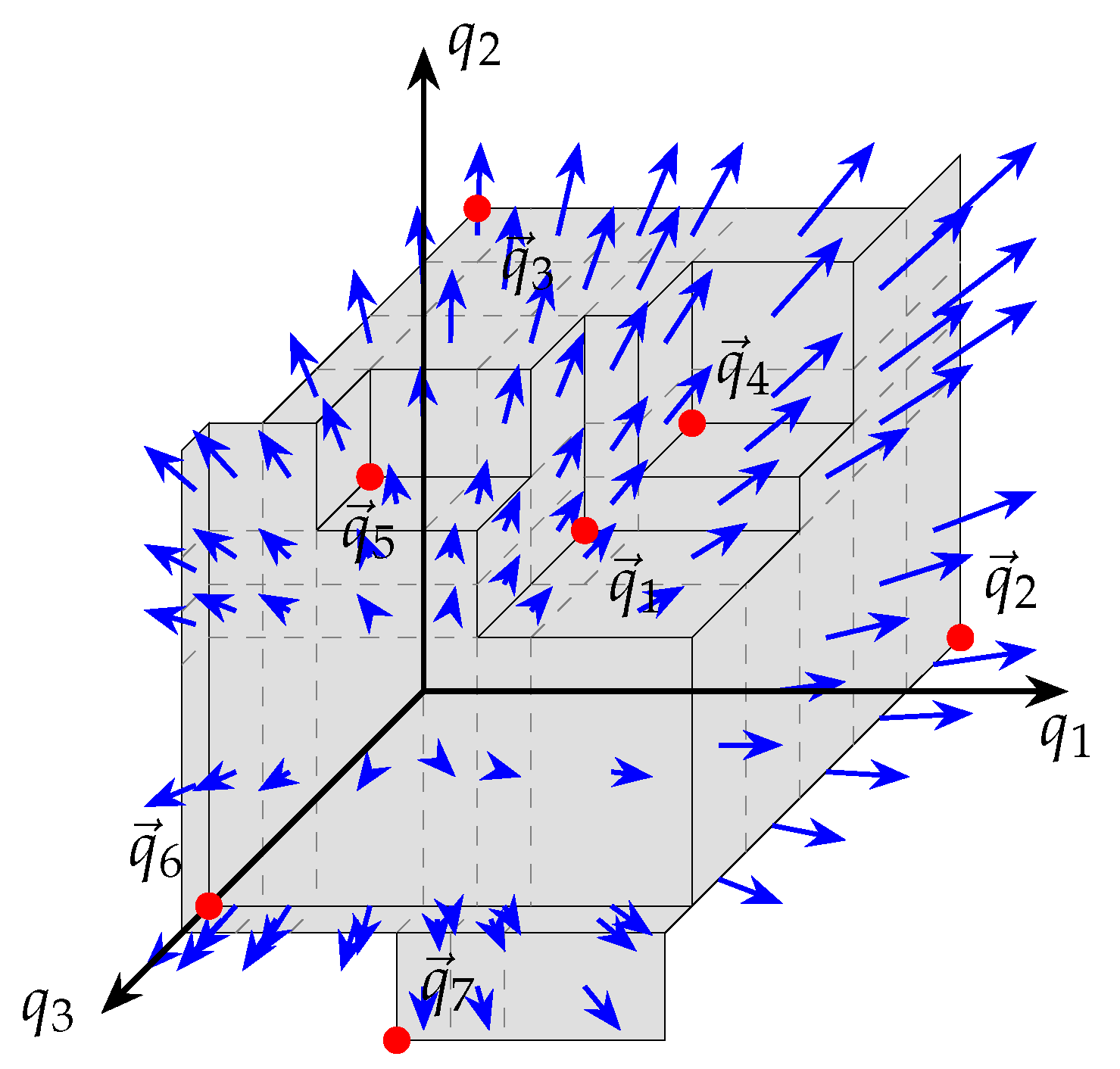
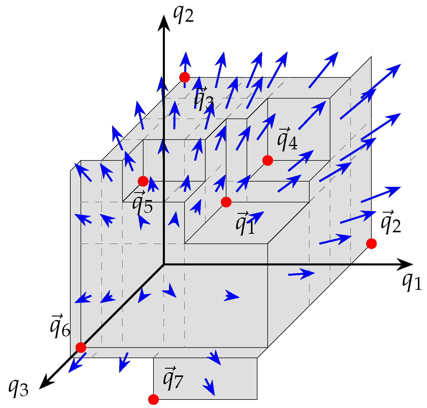
Figure 13 depicts an attainment surface with subdivisions and intersection vectors generated using the naive approach. The porcupine measure’s name is derived from the fact that the intersection vectors resembles the spikes of a porcupine.

Figure 13. A 3-dimensional attainment surface with naive subdivisions and intersection vectors.

6.3. Porcupine Measure (Optimized Implementation)

The large number of subdivisions that result from using the naive implementation of the porcupine measure creates a computationally complex problem when performing the statistical calculations required by the porcupine measure. To reduce the computational cost of the porcupine measure, the naive implementation can be optimized by subdividing the attainment surface only as necessary to accommodate the shape of the attainment surface. Figure 14 depicts an attainment surface with the subdivision lines (dashed) as generated by the optimized implementation.

Figure 14. A 3-dimensional attainment surface with optimized subdivisions.

Note that the algorithm yields the minimum number of subdivisions such that the results are independent of the dimension ordering of the Pareto-optimal points. This is by design to allow for the reproducibility and increased stability of the results.

The optimized implementation of the porcupine measure is summarized in Algorithm 6. For a more detailed algorithm listing, please refer to Appendix B.

Similar to the naive implementation, the porcupine measure is defined as the weighted sum of the intersection lines where a statistically significant difference exists over the sum of all the weights (the percentage of the surface area of the attainment surface, as determined by the weights, where one algorithm statistically performs superior to another).

Figure 15 depicts an attainment surface with subdivisions and intersection vectors generated using the optimized implementation. As can be seen in the figure, the optimized implementation resulted in notably fewer subdivisions and intersection vectors. The lower number of intersection vectors considerably reduces the computational complexity of the measure.

Figure 15. A 3-dimensional attainment surface with optimized subdivisions and intersection vectors.

6.4. Stability Analysis

In order to show that the optimized implementation provides results similar to the naive implementation, 30 independent runs of each measure were executed. Each measurement run calculated the porcupine measure using the approximated POFs as calculated by 30 independent runs of each of the algorithms being compared. A total of $30\times 30=900$ runs were executed for each algorithm being compared.

Table 6 lists the results for the algorithm pairs that were compared. The algorithm pairs are listed without a separator line between them. The results should thus be interpreted by looking at both lines of the comparison. For each algorithm, the mean, standard deviation ($\sigma$), minimum, and maximum for the naive and optimized implementations of the porcupine measure with a maximum side length of $0.1$ are listed.

Table 6. Naive vs. optimized porcupine measure (3-objective WFG problem set).

Problem	Algorithm	Naive				Optimized
		Mean	$\mathit{\sigma }$	Min	Max	Mean	$\mathit{\sigma }$	Min	Max
WFG1	OMOPSO	3.054	2.178	0.2596	9.4	3.092	2.245	0.5106	9.728
	SMPSO	32.34	6.054	17.29	43.92	32.38	6.132	16.57	42.92
	OMOPSO	1.308	1.11	0.2418	4.886	1.32	1.153	0.2445	5.071
	VEPSO	43.55	4.06	30.43	52.71	43.16	4.031	32.27	52.73
	VEPSO	19.62	6.619	8.857	47.63	18.73	4.149	8.679	28.34
	SMPSO	6.631	2.949	0.8017	17.61	6.701	2.782	3.491	17.05
WFG2	OMOPSO	49.88	6.116	32.83	60.57	49.29	6.517	30.85	60.54
	SMPSO	0.01869	0.06869	0.0	0.3711	0.01736	0.06466	0.0	0.3442
	OMOPSO	59.43	4.403	47.63	67.35	59.64	4.397	47.61	66.87
	VEPSO	0.0	0.0	0.0	0.0	0.0	0.0	0.0	0.0
	VEPSO	0.0	0.0	0.0	0.0	0.0	0.0	0.0	0.0
	SMPSO	59.76	4.612	46.3	66.91	59.83	4.716	46.26	67.61
WFG3	OMOPSO	26.98	4.088	18.44	37.32	28.99	4.524	20.43	43.72
	SMPSO	3.099	2.262	0.1569	8.927	3.078	2.097	0.2126	7.497
	OMOPSO	62.55	3.341	55.16	68.42	66.07	3.722	58.36	73.14
	VEPSO	0.5199	0.1456	0.2931	0.8233	0.5875	0.1695	0.2527	0.8897
	VEPSO	1.177	0.48	0.2131	2.315	1.243	0.5278	0.2095	2.5
	SMPSO	59.17	3.402	52.04	64.47	62.57	3.668	55.66	69.12
WFG4	OMOPSO	26.78	2.433	22.7	30.65	26.37	2.919	20.3	31.05
	SMPSO	9.348	1.915	5.002	13.57	9.306	1.989	5.122	13.62
	OMOPSO	63.0	4.539	55.21	75.74	63.82	4.798	55.75	77.11
	VEPSO	0.02337	0.03589	0.0	0.1569	0.02468	0.04244	0.0	0.1929
	VEPSO	0.02615	0.09773	0.0	0.533	0.02406	0.08814	0.0	0.4763
	SMPSO	71.11	3.919	62.78	80.38	71.92	4.072	63.2	82.07
WFG5	OMOPSO	25.67	4.393	17.47	34.0	25.79	4.472	17.55	34.4
	SMPSO	17.61	3.64	11.16	27.63	17.65	3.824	10.68	27.83
	OMOPSO	26.21	2.314	22.2	30.72	26.31	2.432	21.48	31.12
	VEPSO	17.94	2.65	10.6	22.42	17.54	2.691	10.56	21.72
	VEPSO	25.13	4.301	14.71	33.27	25.12	4.463	13.9	33.76
	SMPSO	5.143	1.277	2.736	8.069	5.187	1.338	2.539	8.049
WFG6	OMOPSO	10.21	2.398	6.651	15.76	10.55	2.356	7.035	15.89
	SMPSO	45.3	3.61	37.82	53.57	45.62	3.754	38.12	54.17
	OMOPSO	11.93	4.704	6.098	22.65	12.29	4.854	5.991	23.65
	VEPSO	16.05	5.158	5.421	25.88	16.53	5.414	5.566	26.5
	VEPSO	1.02	0.8952	0.01929	3.795	1.046	0.9204	0.007599	3.983
	SMPSO	20.61	6.907	8.904	37.24	20.94	7.022	8.945	37.69
WFG7	OMOPSO	38.86	3.64	31.77	44.27	39.28	3.516	32.12	44.38
	SMPSO	3.892	0.9721	1.684	5.522	3.888	1.018	1.641	5.507
	OMOPSO	74.41	2.681	67.75	78.68	74.72	2.743	67.8	79.15
	VEPSO	0.0	0.0	0.0	0.0	0.0	0.0	0.0	0.0
	VEPSO	0.001361	0.007456	0.0	0.04084	$9.506\times {10}^{-5}$	0.0005206	0.0	0.002852
	SMPSO	73.39	2.598	68.5	77.94	73.69	2.682	68.92	79.15
WFG8	OMOPSO	41.21	4.789	31.08	49.28	41.55	4.954	30.95	49.24
	SMPSO	3.049	0.948	1.443	5.066	3.106	0.9568	1.54	5.088
	OMOPSO	70.18	3.918	63.04	77.36	70.49	3.847	63.4	77.46
	VEPSO	$6.884\times {10}^{-5}$	0.0002857	0.0	0.001467	0.0	0.0	0.0	0.0
	VEPSO	0.1489	0.2362	0.0	1.023	0.1458	0.223	0.0	0.869
	SMPSO	62.88	3.841	56.14	72.58	63.15	3.861	56.65	73.03
WFG9	OMOPSO	15.89	2.462	11.12	21.29	15.87	2.47	11.48	21.66
	SMPSO	37.58	3.03	32.14	43.94	37.68	3.048	31.95	44.27
	OMOPSO	20.7	2.526	16.86	25.28	20.61	2.515	16.9	26.05
	VEPSO	23.59	1.801	19.21	26.88	24.0	1.795	19.61	27.51
	VEPSO	1.206	0.7576	0.2238	3.162	1.219	0.8411	0.2526	3.605
	SMPSO	21.91	5.093	12.24	31.96	21.8	5.307	11.12	32.25

The experimental results in [22] show that a maximum side length of $0.1$ for the optimized implementation yielded a good trade-off between accuracy of the results and performance when compared with the naive implementation.

Statistical testing was performed to determine if there were any statistically significant differences between the naive and optimized implementations’ results. The Mann–Whitney U test was used at a significance level of $\alpha =0.05$. The purpose of the statistical testing was to determine if there was any information loss due to using the optimized implementation compared to the naive implementation. The results indicated that for 52 out of the 54 measurements, or $96\%$, there were no statistically significant differences. Only for two cases, namely the OMOPSO in the WFG3 OMOPSO vs. VEPSO comparison and the SMPSO in the WFG3 VEPSO vs. SMPSO comparison, was a statistically significant difference noted. In spite of the statistical difference, the ranking of the algorithms did not change. Based on the results, it can, therefore, be concluded that the optimized implementation yielded the same results as the naive implementation and no information was lost. Because no information was lost when using the optimized implementation, it can be concluded that the optimized implementation, with less computational complexity when compared to the naive implementation, can be used when conducting comparisons of multi-objective algorithms.

Algorithm 6 Porcupine measure (optimized implementation).

1: Input: The found POF   2: Output: The porcupine attainment surface   3: Let ${\overrightarrow{q}}_{max}$ be the nadir vector defined as $(max\{q_{s1}\},max\{q_{s2}\},\dots ,max\{q_{sM}\})$ for each of the known Pareto-optimal points, ${\overrightarrow{q}}_s$, of dimension M   4: for each of the objective space basis vectors, $m_c$, do   5:    Project the attainment surface parallel to the basis vector, $m_c$, onto the orthogonal $(M-1)$-dimensional subspace   6:    for each of the Pareto-optimal points, ${\overrightarrow{q}}_s$ do,   7:      Let $\overrightarrow{\widehat{q}}$ be the vector with dimensional values set to the minimum dimensional values that are dominated or the corresponding $q_{max}$ value if no minimum exists   8:      Let $\widehat{Q}$ be the set of all points that dominate $\overrightarrow{\widehat{q}}$ but not ${\overrightarrow{q}}_s$, filtered for non-dominance   9:      for each dimension m do, 10:         Let $Q_m$ be the set of all the m’th dimensional values of the points in $\widehat{Q}$ that fall inside the range $[q_{sm},{\widehat{q}}_m]$ 11:      end for 12:      Let $Q_{min}$ be the set of all the minimum points that will affect the calculation of $\overrightarrow{p}$ 13:      Let $Q_{max}$ be the set of all the maximum points that will affect the calculation of $\overrightarrow{p}$ 14:      Add all dimensional values of the points in $Q_{min}$ and $Q_{max}$ that fall inside the range $[q_{sm},{\widehat{q}}_m]$ to the corresponding $Q_m$ set 15:      Add additional values to the $Q_m$ sets to limit the side lengths to ${\mathsf{\Delta }}_{max}$ 16:      Subdivide the projected attainment surface in each of the m dimensions at every value in the $Q_m$ set into hyper-rectangles 17:      for each hyper-rectangle do, 18:         Let $\overrightarrow{c}$ be the center point of the hyper-rectangle 19:         Let w be the weight of the hyper-rectangle, equal to the product of the hyper-rectangle’s edge lengths 20:         for each dimension m do 21:             Let ${min}_m$ be the smallest of the mth-dimensional values of all the Pareto-optimal points where at least one other dimensional value is less than or equal to that of the corresponding center vector’s dimensional value 22:           Let ${max}_m$ is the largest of the mth-dimensional values of all the Pareto-optimal points 23:         end for 24:         Let $\overrightarrow{p}$ be the intersection vector, calculated as $p_m=\frac{c_m-{min}_m}{{max}_m-{min}_m}$, where $p_m$ is the mth component of the vector $\overrightarrow{p}$ 25:         drawIntersectionLineWithWeight (from = $\mathbf{c}-\mathbf{p}$, to = $\mathbf{c}+\mathbf{p}$, weight = w) 26:      end for 27:    end for 28: end for

The mean standard deviation was $2.743$, and the maximum standard deviation was $7.022$. The conclusion that can be drawn from the data is that the optimized implementation of the porcupine measure is very robust because measurement values for each of the samples were close to the average.

For the experimentation that was carried out for this study, the runtime of the optimized implementation was notably faster than that of the naive implementation. A difference on the orders of a few magnitudes was noticeable.

The computational complexity of the naive implementation is directly proportional to the size of the $Q_m$ sets. It should be noted that, for the tested algorithms with an approximated POF size of 50 points tested over 30 independent samples, the optimal POF had a typical size of 1250 points. The size of the $Q_m$ sets were thus approximately 1250 points. For three dimensions, this resulted in a minimum computational complexity of at least ${1250}^3$, or rather 1,953,125,000 (almost two billion). The optimized implementation resulted in much-reduced computational complexity because only the necessary subdivisions were made. The size of the $Q_m$ sets were much smaller. For the three-dimensional case, the maximum edge length leads to a minimum complexity of at least ${(\frac{1}{0.1})}^3$, or rather 1000 times lower than that of the naive version.

7. Conclusions

This article investigated shortcomings that may have led to the lack of adoption of attainment-surface-based quantitative performance measurements for multi-objective optimization algorithms. It was shown that the quantitative measure proposed by Knowles and Corne was biased against convex Pareto-optimal fronts (POFs) when using rotational intersection lines. The attainment-surface-shaped intersection lines (ASSIL) generation approach was proposed. The ASSIL generation approach was shown not to be biased against any attainment surface shape.

An algorithm for an M-dimensional attainment-surface-based quantitative measure, named the porcupine measure, was presented. Additionally, a computationally optimized implementation of the porcupine measure was introduced and analyzed. The results indicated that the optimized implementation performed as well as the naive implementation.

The porcupine measure allows for a quantitative comparison between M-dimensional approximated POFs through the use of attainment surfaces. The porcupine measure provides additional information on an algorithm’s performance when compared to another algorithm, which was previously not quantifiable. A thorough comparison comparing the state-of-the-art multi-objective optimization algorithms using the porcupine measure is left as future work.