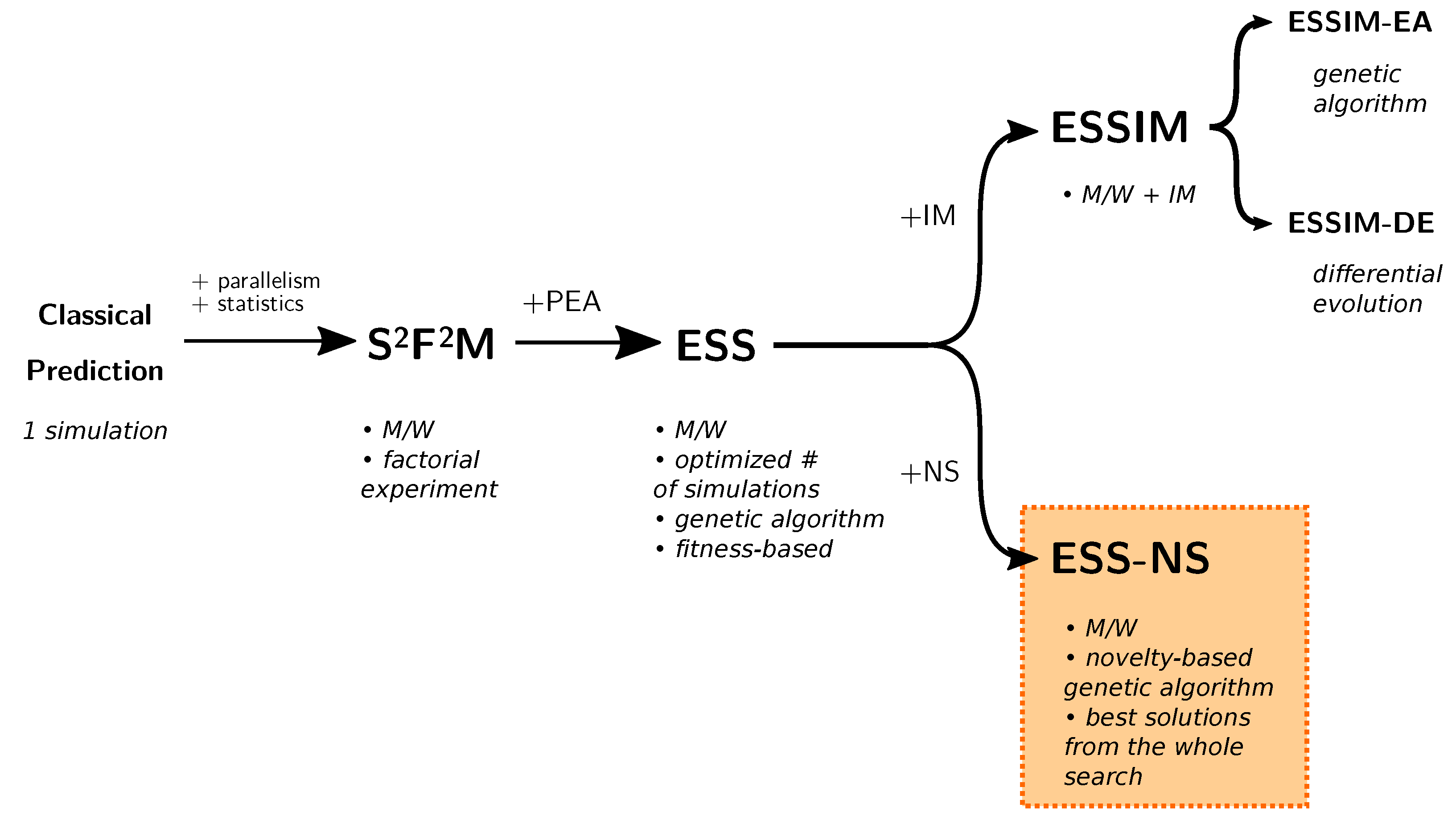
Article

Evolutionary Statistical System Based on Novelty Search: A Parallel Metaheuristic for Uncertainty Reduction Applied to Wildfire Spread Prediction

by
Jan Strappa
1,2,*,
Paola Caymes-Scutari
1,2 and
Germán Bianchini
2
1
Consejo Nacional de Investigaciones Científicas y Técnicas—Centro Científico Tecnológico Mendoza (CONICET, CCT-Mendoza), Mendoza 5500, Argentina
2
Laboratorio de Investigación en Cómputo Paralelo/Distribuido (LICPaD), Facultad Regional Mendoza, Universidad Tecnológica Nacional, Mendoza 5500, Argentina
*
Author to whom correspondence should be addressed.
Algorithms 2022, 15(12), 478; https://doi.org/10.3390/a15120478
Submission received: 14 October 2022 / Revised: 30 November 2022 / Accepted: 9 December 2022 / Published: 15 December 2022
(This article belongs to the Special Issue Parallel/Distributed Combinatorics and Optimization)

Abstract

:
The problem of wildfire spread prediction presents a high degree of complexity due in large part to the limitations for providing accurate input parameters in real time (e.g., wind speed, temperature, moisture of the soil, etc.). This uncertainty in the environmental values has led to the development of computational methods that search the space of possible combinations of parameters (also called scenarios) in order to obtain better predictions. State-of-the-art methods are based on parallel optimization strategies that use a fitness function to guide this search. Moreover, the resulting predictions are based on a combination of multiple solutions from the space of scenarios. These methods have improved the quality of classical predictions; however, they have some limitations, such as premature convergence. In this work, we evaluate a new proposal for the optimization of scenarios that follows the Novelty Search paradigm. Novelty-based algorithms replace the objective function by a measure of the novelty of the solutions, which allows the search to generate solutions that are novel (in their behavior space) with respect to previously evaluated solutions. This approach avoids local optima and maximizes exploration. Our method, Evolutionary Statistical System based on Novelty Search (ESS-NS), outperforms the quality obtained by its competitors in our experiments. Execution times are faster than other methods for almost all cases. Lastly, several lines of future work are provided in order to significantly improve these results.

1. Introduction

The prediction of propagation of natural phenomena is a highly challenging task with important applications, such as prevention and monitoring of the behavior of forest fires, which affect millions of hectares worldwide every year, with devastating consequences on flora and fauna, as well as human health, activities, and economy [1]. In most cases, forest fires are human-caused, although there are also natural causes, such as lightning, droughts, or heat waves. Additionally, climate change has effects, such as high temperatures or extreme droughts, that exacerbate the risk of fires. The prevalence of these phenomena makes it crucial to have methods that can aid with firefighting efforts, e.g., prevention of fires and monitoring and analysis of fire spread on the ground. A basic tool for these analyses are fire simulators, which use computational propagation models in order to predict how the fire line progresses during a period of time. Examples of simulators are BEHAVE [2], FARSITE [3], fireLib [4], BehavePlus [5], and FireStation [6]. Fire spread prediction tasks can be performed either in real time or as a precautionary measure, for example, in order to assess areas of higher risk, or for the development of contingency plans that allocate resources according to predicted patterns of behavior.
Unfortunately, the propagation models for fire spread prediction involve a high degree of uncertainty. On the one hand, modelling natural phenomena involves the possibility of errors due to characteristics inherent to the computational methods used. On the other hand, the simulators require the definition of a number of environmental parameters, also called a scenario, and although these values can greatly influence the results of a prediction, they are often not known beforehand, cannot be provided in real time, or may be susceptible to measuring errors. These difficulties result in predictions that may be far from the actual spread, especially when using what we call a “classical prediction”, i.e., a single prediction obtained by simulating the fire with only one set of parameters.
Nowadays, there are several frameworks that follow strategies for reducing this uncertainty based on the combination of results from multiple simulations. There are solutions categorized as Data-Driven Methods (DDMs), which perform a number of simulations taking different scenarios as input. From these results, the system chooses the set of parameters that obtained a better prediction in the past and uses it as input for the prediction of the future behavior of the fire. Examples of this strategy are found in [7,8]. While there is an improvement over the single-simulation strategy, these methods still use a single scenario for the prediction. This can be a great limitation due to the uncertainty in the dynamic conditions of the fire, and the possibility of errors; that is, a good scenario for a previous step might not be as good for the next. For example, a scenario might have yielded good results only by chance, or it may be an anomalous case that does not generalize well to the fire progress.
Other approaches have set out to overcome this problem by combining results from multiple simulations and using these combined results for producing a prediction. Such methods are called Data-Driven Methods with Multiple Overlapping Solutions, or DDM-MOS. We provide a summary of the taxonomy of several methods in Figure 1. Except for the Classical Prediction, all methods shown in the figure belong in the DDM-MOS category. One of these solutions is the Statistical System for Forest Fire Management, or S 2 F 2 M [9]. This system uses a factorial experiment of the values of variables for choosing scenarios to evaluate, which consists of an exhaustive combination of values based on a discretization of the environmental variables. This strategy presents the challenge of having to deal with a large space of possible scenarios, which makes simulation prohibitive. In order to produce acceptable results in a feasible time, other methods introduced the idea of performing a search over this space in order to reduce the sample space considered for the simulations. One of the frameworks that follow this strategy is the Evolutionary Statistical System (ESS) [10], which embeds an evolutionary algorithm for the optimization of scenarios in order to find the best candidates for predicting future propagation. Recently, other proposals based on ESS have been developed: ESSIM-EA [11,12] and ESSIM-DE [13]. These systems use Parallel Evolutionary Algorithms (PEAs) with an Island Model hierarchy: a Genetic Algorithm [14,15], and Differential Evolution [16], respectively. The optimization performed by these methods was able to outperform previous approaches, but it presented several limitations. The three frameworks mentioned use evolutionary algorithms that are based on a process that iteratively modifies a “population” of scenarios by evaluating them according to a fitness function. In this case, the fitness function compares the simulation with the real fire progress. For problems with high degrees of uncertainty, the fitness function may present features that hinder the search process and might prevent the optimization from reaching the best solutions [17]. Another limitation that becomes relevant in this work is that the state-of-the-art methods ESS, ESSIM-EA, and ESSIM-DE use techniques that were designed with the objective of converging to a single solution, which might negate the benefits of using multiple solutions if the results to be overlapped are too similar to each other.
In this work, we propose and evaluate a new method for the optimization of scenarios. Our method avoids the issues of previous works by using a different criterion for guiding the search: the Novelty Search (NS) paradigm [18,19,20]. NS is an alternative approach that ignores the objective as a guide for exploration and instead rewards candidate solutions that exhibit novel (different from previously discovered) behaviors in order to maximize exploration and avoid local optima and other issues related to objective-based algorithms. In an early work [21], we presented the preliminary design of a new framework based on ESS that incorporated the Novelty Search paradigm as the search strategy for the optimization of scenarios. This article is an extended work whose main contributions are the experimental results and their corresponding discussion. These results comprise two sets of experiments: one for the calibration of our method and another for the comparison of our method against other state-of-the-art methods. In addition, we have made some corrections in the pseudocode, reflecting the final implementation that was evaluated in the experiments. Our experimental results support the idea that the application of a novelty-based metaheuristic to the fire propagation prediction problem can obtain comparable or better results in quality with respect to existing methods. Furthermore, the execution times of our method are better than its competitors in most cases. To the best of our knowledge, this is the first application of NS as a parallel genetic algorithm and also the first application of NS in the area of propagation phenomena.
In the next section, we guide the reader throughout previous works related to our present contribution; firstly, in the area of DDM-MOS, with a detailed explanation of existing systems (Section 2.1 and Section 2.2), and secondly, in the field of NS (Section 2.3), where we explain the paradigm and its contributions in general terms. Then, in Section 3, we present a detailed description of the current contribution and provide a pseudocode of the optimization algorithm. Section 4 presents the experimental methods, results, and discussion. Finally, in Section 5, we detail our main conclusions and describe possible lines of future work. In addition, Appendix A presents a static calibration experiment performed on our method.

2. Related Works

In this section, first we summarize the operation and previous results of the competitor systems against which our new method was compared. These competitors are a subset of the taxonomy presented in Section 1 (Figure 1). We begin in Section 2.1 with a general outline of the system on which our novel method is based, i.e., ESS, and then, in Section 2.2, we delve into the most recent proposals, i.e., ESSIM-EA and ESSIM-DE, which are also based on ESS. Finally, in Section 2.3, we present the main concepts and related works in the area of Novelty Search.

2.1. ESS Framework

The systems referred to in this paper fit into the DDM-MOS category, given that they perform multiple simulations, each based on a different scenario, and rely on a number of simulations in order to yield a fire spread prediction. Previous approaches showed limitations, either caused by the use of a single simulation for the predictions or by the complexity of considering a large space of possibilities, which includes redundant or unfeasible scenarios. To overcome these limitations, the Evolutionary Statistical System (ESS) was developed. Its core idea is to produce a reduced selection of results with the aid of an evolutionary algorithm that searches over the space of all possible scenarios. The objective is to reduce the complexity of the computations while considering a sample of scenarios that may produce better prediction results. In order to understand the scheme of the method proposed in this paper and of its other, more recent competitors, it is necessary to have a general comprehension of how ESS works, since they all share a similar framework.
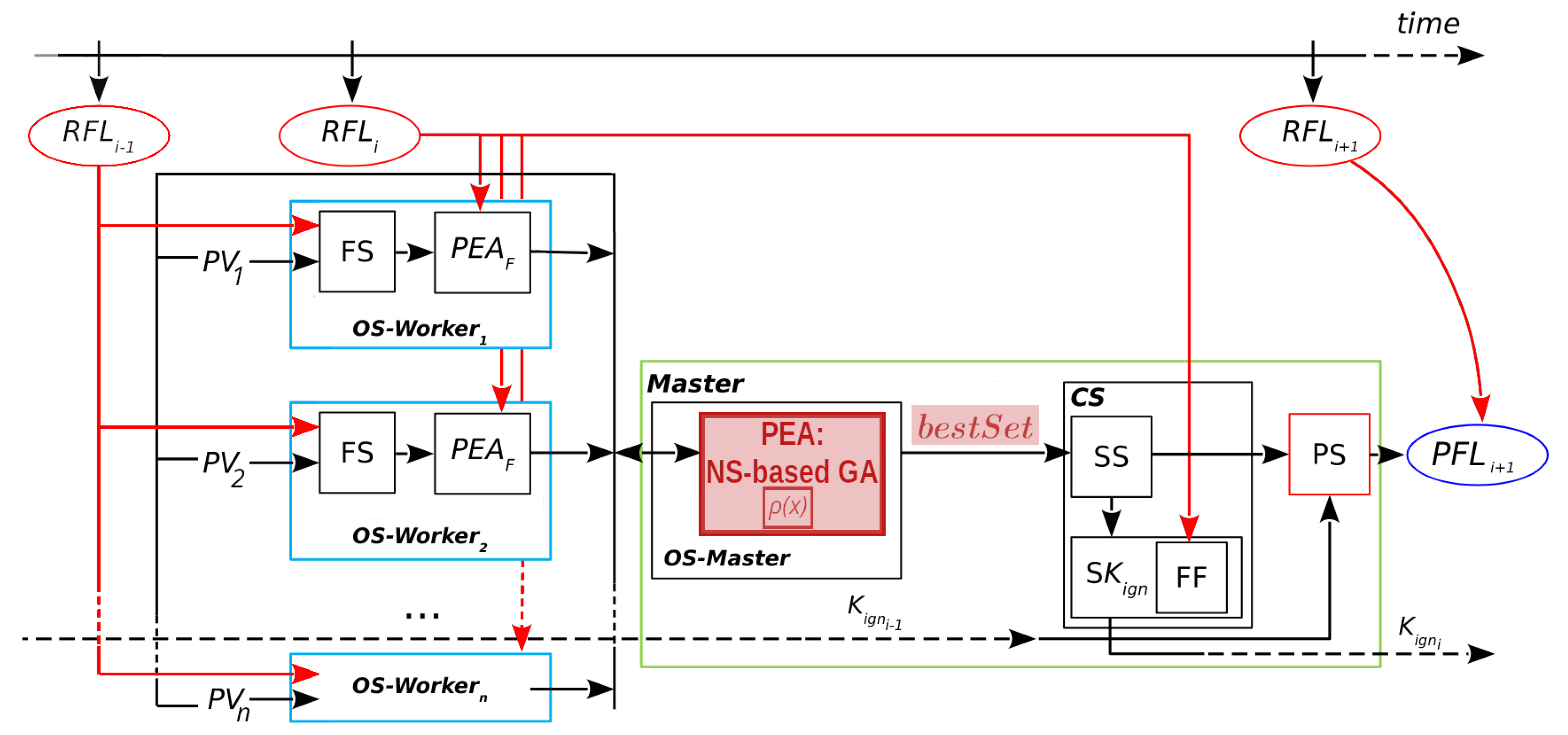
A general scheme of the operation of ESS can be seen in Figure 2 (reproduced and modified with permission from [
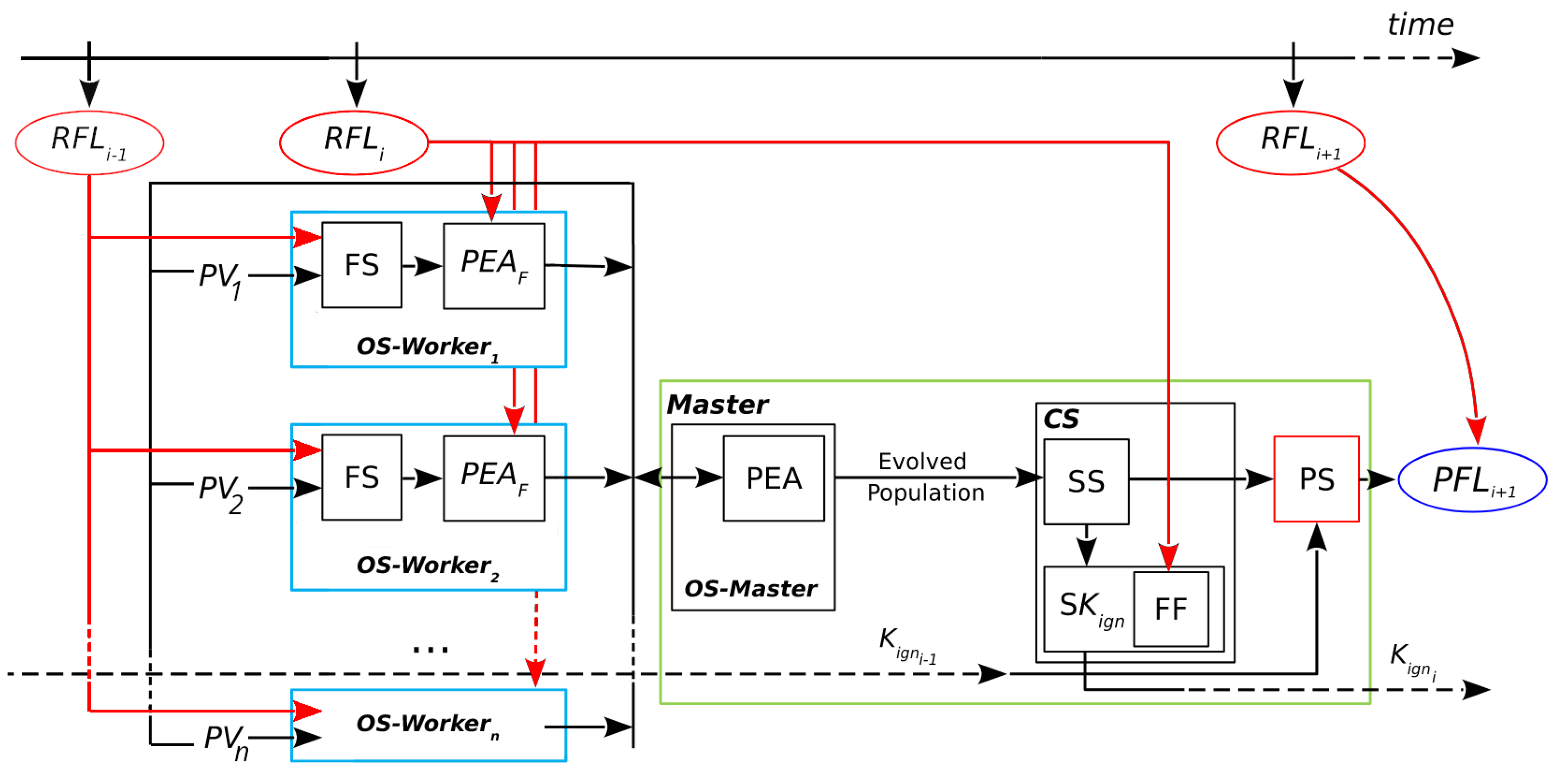
11]). ESS takes advantage of parallelization with the objective of reducing computation times. This is achieved by implementing a Master/Worker parallel hierarchy for carrying out the optimization of scenarios. During the fire, the whole prediction process is repeated for different discrete time instants. These instants are called prediction steps, and in each of them, four main stages take place: Optimization Stage (divided into Master and Workers, respectively: OS-Master and OS-Worker), Statistical Stage (SS), Calibration Stage (CS), and Prediction Stage (PS).
At each prediction step, the process aims to estimate the growth of the fire line from t i to t i + 1 . For every step, a new optimization starts with the OS. This involves a search through the space of scenarios guided by a fitness function. The process is a classic evolutionary algorithm that starts with the initialization of the population, performs the evolution of the population (selection, reproduction, and replacement), and then finishes when a termination condition is reached. This parallel evolutionary process is divided into the Master and Workers, shown in Figure 2 as OS-Master and OS-Worker, respectively. The OS-Master block involves the initialization and modification of the population of scenarios, represented by a set of parameter vectors PV { 1 n } . The Master distributes these scenarios to the Workers processes (shown as P V 1 to P V n ).
The Workers evaluate each scenario that they receive by sending it as input to a fire behavior simulator FS. In the FS block, the information from the Real Fire Line at the previous instant, R F L i 1 , is used together with the scenario to produce a simulated map for that scenario. Then, this simulated map and the information from R F L i are passed into the block P E A F . As represented in the figure, two inputs from the fire line are needed at the OS-Worker (i.e., R F L i 1 and R F L i ): the first one to produce the simulations, and the second one to evaluate the fitness of those simulations. Such evaluations are needed for guiding the search and producing an adequate result for the next stage (the SS). Therefore, the fitness is obtained by comparing the simulated map with the real state of the fire at the last known instant of time. The Master process receives these evaluations (the simulated maps with their fitness) and uses them to continue with the evolution, i.e., to perform selection, reproduction, and replacement of the population.
Although not shown in the figure for clarity, it is important to note that the OS is iterative in two ways. Firstly, the Master must divide all scenarios in the population into a number of vectors according to the number of Worker processes; e.g., if there are 200 scenarios and 50 Workers, the Master must send a different PV (each containing 50 scenarios P V { 1 50 } ) for evaluation four times in order to complete the 200 evaluations. Secondly, the Master will repeat this process for each generation of the P E A until a stopping condition is reached.
Once the OS-Master has finished, the following stages are CS and PS. These stages involve the computation of the overlapped result. For the CS, the general idea is to use a collection of simulated maps resulting from the evolutionary algorithm and produce as output an aggregated map and a threshold value; then, for the PS, a final map is produced as a matrix of burned and unburned cells, and this constitutes the prediction for t n + 1 .
In the case of ESS, the collection of simulated maps is equivalent to the evolved population, and the complete CS is performed by the Master. This is represented by the CS block in Figure 2, which involves several steps. The first step is the Statistical Stage or SS. The purpose of this step is to take into consideration a number of solutions for the prediction. For this, the Master aggregates the resulting maps obtained from the evolved population, producing a matrix in which each cell is the sum of cells that are ignited according to each simulated map from the input. These frequencies are interpreted as probabilities of ignition. Although in this case the selection of maps is straightforward, other criteria can be used to consider different simulations with different results regarding the reduction of uncertainty.
After obtaining this probability matrix, it will be used for two purposes: on the one hand, it is provided as input for the PS; on the other hand, it is used in the next step of the CS: the search for the Key Ignition Value, or K i g n . This is a simple search represented by the block S K i g n . These two parts are interrelated: the PS at t n + 1 depends on the output of the CS at t n , which is K i g n n . Up to this point, we have a probability map, but the predicted fire line P F L 
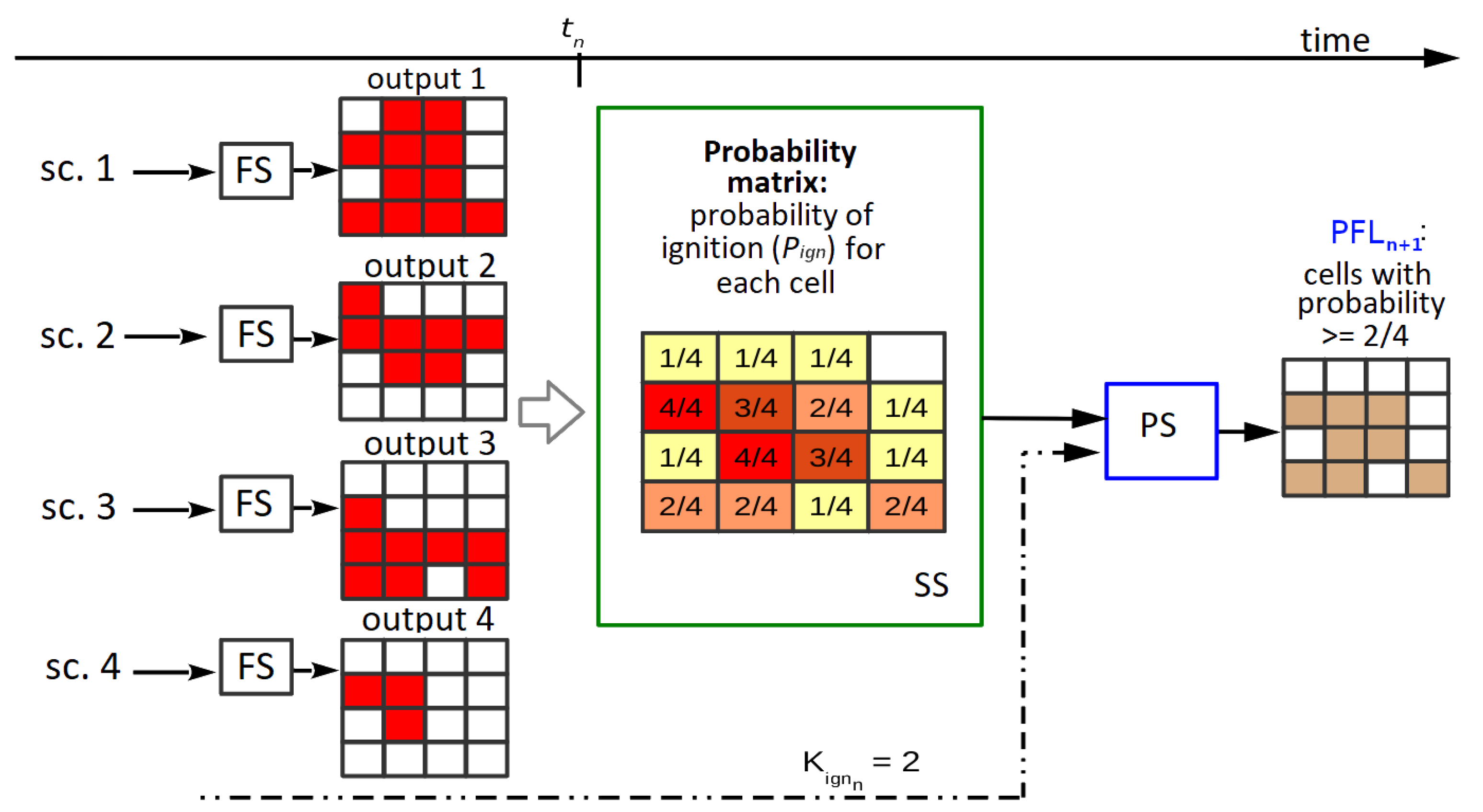
consists of cells that are marked as either burned or unburned. Then, we need a threshold for establishing which cells of the probability map are going to be considered as ignited. In other words, the threshold establishes how many simulated maps must have each cell as ignited in order for that cell to appear as ignited in the final map. A more detailed diagram of the first use of the matrix is illustrated in Figure 3 (reproduced, modified, and translated with permission from [22]). In the example from this figure, if there are four simulated maps and K i g n = 2 , then for a cell to be predicted as burned in the aggregated map, it must be present as such in at least two of the simulated maps. Note that instead of being the result of one simulation, this final map, P F L n + 1 (shown at the right in Figure 3, after the PS), aggregates information from the collection of simulated maps obtained as the output of the OS (simplified in the l.h.s. of the figure). In order to choose an appropriate value of K i g n , it is assumed that a value that was found to be a good predictor for the current known fire line will still be a reasonable choice for the next step due to the fact that propagation phenomena have certain regularities. Therefore, the search for this value involves evaluating the fitness of different maps generated with different threshold values. Going back to Figure 2, the fitness is computed between each of these maps and the R F L i in the F F block. For the PS to take place at a given prediction step, the best K i g n must have been found at the previous iteration. This is represented by the arrows going from the previous iteration into the PS ( K i g n i 1 ) and from S K i g n towards the next iteration ( K i g n i ). For instance, at step t 2 , the value K i g n 2 is chosen to be used within the PS of t 3 . The CS begins in the second fire instant since it depends on the knowledge of the real fire line at the first instant. Once the first result from the calibration has been obtained, that is, starting from the third fire instant, then a prediction from the aggregated map can be obtained.
After each prediction step, and when the R F L is known for that step, the P F L can be compared if needed. For this, one can once again use the fitness function, this time in order to evaluate the final predictions (represented by the connection between R F L i + 1 and P F L i + 1 ). In our experiments, this evaluation is performed statically after each complete run, given that the cases under consideration are controlled fires for which the R F L is known for all steps. A real-time evaluation could also be achieved by computing this fitness iteratively after obtaining the R F L for the previous instant and after each prediction map has been obtained.

2.2. ESSIM-EA and ESSIM-DE Frameworks

This section summarizes the operation of the more recently developed systems, ESSIM-EA and ESSIM-DE, which are both based on ESS and are also included in our comparison against our new method in Section 4.
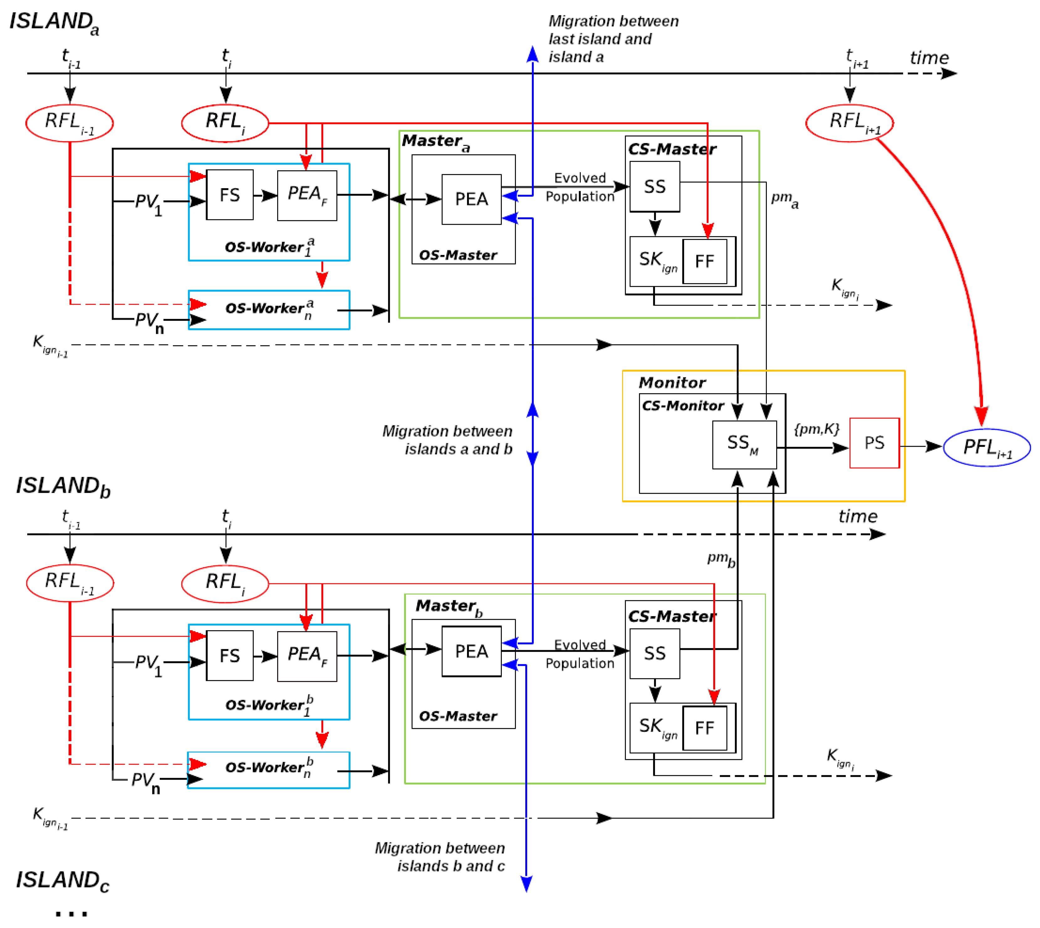
ESSIM-EA stands for Evolutionary Statistical System with Island Model based on evolutionary algorithms, while ESSIM-DE is ESSIM based on Differential Evolution. Both systems fit into the category of DDM-MOS, since they employ a method for selecting multiple solutions from the space of possible scenarios and producing an overlapped result in order to perform the prediction of fire propagation.
ESSIM-EA and ESSIM-DE are summarized in Figure 4, reproduced and modified from [11] (Published under a Creative Commons Attribution-NonCommercial-No Derivatives License (CC BY NC ND). See https://creativecommons.org/licenses/by-nc-nd/4.0/, accessed on 13 October 2022). The four main stages in these systems are the same as in ESS: Optimization Stage (OS), Statistical Stage (SS), Calibration Stage (CS), and Prediction Stage (PS). Because both ESSIM systems use a hierarchical scheme of processes, these stages are subdivided to carry out the different processes in the hierarchy. The Master/Worker hierarchy of ESS is augmented with a more complex hierarchy that consists of one Monitor, which handles multiple Masters, and, in turn, each Master manages a number of Workers. Essentially, the system uses a number of islands where each island implements a Master/Worker scheme; the Monitor then acts as the Master process for the Masters of the islands. On each island, the Master/Worker process operates as described in Section 2.1 for ESS: the Master distributes scenarios among the Workers for performing the simulations in the OS.
The process begins with the Monitor, which sends the initial information to each island to carry out the different stages. The Master process of each island performs the OS: it controls the evolution of its population and the migration process. On each island during each iteration of the evolutionary algorithm, the Master sends individuals to the Worker processes, which are in charge of their evaluation. For more details on the operation of the island model, see [11].
After the evolutionary process, the SS takes place in which the Master performs the computation of the probability matrix that is required for the CS and PS. In this new scheme, the SS is carried out by the Master, the CS is performed by both the Master and the Monitor, and the PS is handled only by the Monitor. The CS starts with the CS-Master block, where each Master generates a probability matrix and provides its K i g n value. The block CS-Monitor represents the final part of the calibration in which the Monitor receives all matrices sent by the Masters and then selects the best candidate based on their fitness (these fitness values have already been computed by the Masters). The matrix selected by the Monitor is used for producing the current step prediction.
Experimentally, when ESSIM-EA was introduced, it was shown to be able to reach predictions of similar or higher quality than ESS but with a higher cost in execution times. Later, ESSIM-DE was developed, and it significantly reduced response times, but the quality did not improve in general. Subsequent works have improved the performance of the ESSIM-DE method by embedding tuning strategies into the process [23]. Tuning strategies are methods for improving the performance of an application by calibrating critical aspects. Application tuning can be automatic (when the techniques are transparently incorporated in the application) and/or dynamic (adjustments occur during execution) [24]. For ESSIM-DE, there are two automatic and dynamic tuning metrics which have been shown to mitigate the issues of premature convergence and population stagnation present in the case of application of the algorithm. One metric is a population restart operator [13], and the other involves the analysis of the IQR factor of the population throughout generations [25]. The results showed that ESSIM-DE enhanced with these metrics achieved better quality and response times with respect to the same method without tuning.
Even though the two approaches described provide improvements over ESS, they are still limited in several fundamental aspects. The first aspect has to do with the design of the metaheuristics that were adapted for use in the OS of the ESSIM systems. These are population-based algorithms that are traditionally used with the objective of selecting a single solution: the best individual from the final population, obtained from the last iteration of the evolution process. Instead, the adaptations implemented use the final population to select a set of solutions for the CS and PS. Since evolutionary metaheuristics tend to converge to a population of similar genotypes, that is, of individuals which are similar in their representation, the population evolved for each prediction step may consist of a set of scenarios that are similar to each other and therefore produce similar simulations. This may be a limiting factor for the uncertainty reduction objective. To understand this, it must be noted that complex problems do not usually have a smooth fitness landscape, which may imply that individuals that are genotypically far apart in the search space may still have acceptable fitness values and could be valuable solutions. Thus, the metaheuristics implemented in the ESSIM systems may leave out these promising candidates. The second aspect is that in the case of ESSIM-DE, the baseline version performs worse than ESS and ESSIM-EA with respect to quality, which led to the design of the previously mentioned tuning mechanisms. These variants produced better results in quality than the original version of ESSIM-DE but did not significantly outperform ESSIM-EA. Such findings seem to support the idea that this particular application problem could benefit from a greater exploration power, combined with a strategy that could take better advantage of the solutions found during the search. From this reasoning, we arrived at the idea of applying a paradigm that maximizes exploration, while keeping solutions in a way that is compatible by design with a DDM-MOS, that is, a system that is based on multiple overlapped solutions.

2.3. Novelty Search: Paradigm and Applications

The limitations observed in existing systems led us to consider the selection of other search approaches that may yield improvements in the quality of predictions. Given the particular problems observed in the experimental results of previous works, we determined that a promising approach for this problem could be the Novelty Search (NS) paradigm. In this section, we explain the main ideas and describe related works behind this approach.
Metaheuristic search algorithms reward the degree of progress toward a solution, measured by an objective function, usually referred to as a score or fitness function depending on the type of algorithm. This function, together with the neighborhood operators of a particular method, produces what is known as the fitness landscape [26]. By changing the algorithm, the fitness function, or both, a given problem may become easier or more difficult to solve, depending on the shape and features of the landscape that they generate. In highly complex problems, the fitness landscape often has features that make the objective function inefficient in guiding the search or may even lead the search away from good solutions [17]. This has led to the creation of alternative strategies that address the limitations inherent to objective-based methods [27]. One of these strategies is NS, introduced in [19]. In this paradigm, the search is driven by a characterization of the behavior of individuals that rewards the dissimilarity of new solutions with respect to other solutions found before. As a consequence, the search process never converges but rather explores many different regions of the space of solutions, which allows the algorithms to discover high fitness solutions that may not be reachable by traditional methods. This exploration power differs from metaheuristic approaches in that it is not driven by randomness, but rather by explicitly searching for novel behaviors. NS has been applied with good results to multiple problems from diverse fields [18,19,28,29,30,31].
Initially, the main area of interest for applications of NS consisted of open-ended problems. In this area, the objective is to generate increasingly complex, novel, or creative behaviors; there is no fixed, predetermined solution to be reached. Interestingly, NS has also been proven useful for optimization problems in general, finding global optima in many cases and outperforming traditional metaheuristics when the problems have the quality of being deceptive, that is, when the combination of solutions of high fitness leads to solutions of lower fitness and vice versa [31].
In order to guide the search by novelty, all algorithms following this paradigm need to implement a function to evaluate the novelty score of the solutions. Therefore, a novelty measure of the solutions must be defined in the space of behaviors of the solutions. This measure, usually called d i s t in the literature, is problem-dependent; an example can be the difference between values of the fitness function of two individuals.
A frequently used novelty score function is the one presented by [19], which, for an individual x, computes the average distance to its k closest neighbors:
ρ ( x ) = 1 k i = 0 k 1 d i s t ( x , μ i ) ,
where μ i is the i-th nearest neighbor of the individual x according to the distance function d i s t . In the literature, the parameter k is usually selected experimentally, but the entire population can also be used [18,32].
To perform this evaluation, it is not sufficient to select close individuals by considering only the current population; it is also necessary to consider the set of individuals that have been novel in past iterations. To this end, the search incorporates an archive of novel solutions that allows it to keep track of the most novel solutions discovered so far and uses it to compute the novelty score. The novelty values obtained are used to guide the search, replacing the traditional fitness-based score. This design allows the search to be unaffected by the fitness function landscape, directly preventing problems such as those found in the systems described in the previous section.
When using conventional metaheuristics, due to the randomness involved in the algorithms, it is possible that some high fitness solutions may be lost in intermediate iterations with no record of them remaining in the final population. In contrast, NS can avoid this issue because when applied to optimization problems it makes use of a memory of the best performing solution(s), as measured, for example, by the fitness function. In this way, even though NS never converges to populations of high fitness, it is possible to keep track of the best solutions (with respect to the fitness function or any characterization of the behavior of the solutions) found throughout the search.
Different metaheuristics have already been implemented using the NS paradigm, such as a Genetic Algorithm [33] and Particle Swarm Optimization [34]. Additionally, multiple hybrid approaches that combine fitness and novelty exist in the literature and have been shown to be effective in solving practical problems. Among some of the approaches used, there are weighted sums between fitness and novelty-based goals [35], different goals in a multi-objective search [36], and independent searches with some type of mutual interaction [29], among others [19,28,30,37,38,39].
Metaheuristics can generally be parallelized in different ways and at different levels. For example, one can run an instance of an algorithm that parallelizes the computation of the fitness function, or one can have a process that manages many instances of the whole algorithm in parallel. The advantages of parallelization are better execution times, more efficient use of resources, and/or improvements in the performance of the algorithm. Just as NS can be implemented by adapting existing metaheuristics to the NS paradigm, existing parallel metaheuristics can also be used as a template for new parallel novelty-based approaches. However, it must be considered that novelty-based criteria, together with the archive mechanism, may warrant additional efforts in order to design an adequate solution. In the particular case of NS, parallelization can be a way to enhance the search, giving it a greater exploration capacity without excessively affecting the execution time. Examples of parallel algorithms containing an NS component can be found in [40,41].

3. Novelty-Based Approach for the Optimization Stage in a Wildfire Prediction System

In this section, we present the new approach in two parts. First, we explain the operation of the general scheme for the new prediction system and how it differs from its predecessors. Second, we describe in detail the novel evolutionary algorithm that is embedded as part of the Optimization Stage in this system.

3.1. New Framework: ESS-NS

The framework that has been implemented for the new method is called Evolutionary Statistical System based on Novelty Search, or ESS-NS. Its general scheme is illustrated by Figure 5. There are several aspects that are analogous with respect to ESS (compare to Figure 2), such as the Master/Worker hierarchy, where Workers carry out the simulations and fitness evaluations while the Master handles the steps of the evolutionary algorithm; stages other than the Optimization Stage remain unchanged. However, the optimization component has important modifications, particularly in the Master process, and these are highlighted in the figure. As its predecessors, this framework consists of a prediction process with the same stages from Figure 2 (Section 2.1): Optimization Stage (OS), Statistical Stage (SS), Calibration Stage (CS), and Prediction Stage (PS).
We have used the same propagation simulator, called fireSim [4], which is implemented in an open-source and portable library, fireLib. This simulator takes the following parameters as input: a terrain ignition map and the set of parameters concerning the environmental conditions and terrain topography. These parameters are described in Table 1. The first row contains the name of the Rothermel Fuel Model, which is a taxonomy describing 13 models of fire propagation commonly used by a number of simulators, including fireSim. The remaining rows represent environmental aspects, such as wind conditions, humidity, slope, etc. For more information on the parameters modeled by this library, see [42]. The output of this simulator is a map that indicates in each cell the estimated time instant of ignition of each cell. If, according to the simulation, the cell is never reached by the fire, it is set to zero. The order and functioning of the Statistical, Calibration, and Prediction stages, in addition to their assignment to Master and Workers, are the same as those presented in Section 2.1.
As for the Optimization Stage, there are two crucial differences from ESS. First, the metaheuristic contained in this stage is also an evolutionary algorithm, but its behavior in this case follows the NS paradigm: the strategy implemented is novelty-based with a genetic algorithm, as shown in the shaded block inside the Master (PEA: NS-based GA) in Figure 5. We defer the details of this algorithm to the following section; however, it is important to note here that this novelty-based method requires an additional computation of a score, that is, the novelty score, represented by the function ρ ( x ) from Equation (1). The second difference is that the output of the optimization algorithm is not the final evolved population, as in previous methods; rather, it is a collection of high fitness individuals which were accumulated during the search, which we call b e s t S e t . Although the need for this structure originates from an apparent limitation of NS, that is, its lack of convergence, this mechanism is in fact an advantage of this method, and it is more suitable to this application problem than the previous methods, which are based on single-solution metaheuristics. The difference lies in that our NS design has the ability to record individuals from completely different areas of the search space and include them in the final aggregated matrix. As discussed in Section 2.2, fitness-based evolutionary algorithms converge to a population of similar individuals, which are redundant, and the evolved population will almost inevitably include some random or not-so-fit individuals (that were generated and selected during the last iteration) that do not contribute to the solution. Since this collection is used for the purposes of reducing uncertainty in the SS, we considered that the advantages of this new design could be an appropriate match for said stage.
It is important to note that ESS-NS differs from the most recent approaches in that it uses the simpler model of Master/Worker (with no islands and only one population). Although the novelty-based strategy performs more steps than the original ESS, the Master process only delegates the simulation and evaluation of individuals to the Workers since this is the most demanding part of the prediction process. Even so, this has not been a problem in our experimentation since the additional steps, such as novelty score computation and updating of sets, do not add significant delays to the execution. The simplification of the parallel hierarchy is motivated by the need to have a baseline algorithm for future comparisons and to be able to analyze the impact of NS alone on the quality of results. Considering that NS uses a strategy that was designed not only to keep diversity and emphasize exploration but to actively seek them, it serves as an alternative route to solve the problem that originally made it necessary to resort to mechanisms such as the island model. Additionally, such a design would require additional mechanisms, for example, for handling the migrations, and these can directly affect both the quality and the efficiency of the method, making it harder to assess the performance of the method. At the moment, these considerations and possible variants are left as future work.

3.2. Novelty-Based Genetic Algorithm with Multiple Solutions

Our proposal consists of applying a novelty-based evolutionary metaheuristic as part of the Optimization Stage of a wildfire prediction system. We have selected a classical genetic algorithm (GA) as the metaheuristic, which has been adapted to the NS paradigm. This choice was made for two reasons: on the one hand, for simplicity of implementation and, on the other hand, for comparative purposes, since existing systems are also based on variants of evolutionary algorithms, and two of them (ESS and ESSIM-DE) use a GA as their optimization method.
The novelty measure selected is computed as in Equation (1). In this context, x is a scenario, and we define d i s t as the difference between the fitness values of each pair of scenarios:
d i s t ( x , μ i ) = | f i t n e s s ( x ) f i t n e s s ( μ i ) | .
For computing this difference, we used the same fitness function as the one used in the ESS system and its successors: the Jaccard Index [43]. It considers the map of the field as a matrix of square cells (which is the representation used by the simulator):
f i t n e s s ( A , B ) = | A B | | A B | ,
where A represents the set of cells in the real map without the subset of burned cells before starting the simulations, and B represents the set of cells in the simulation map without the subset of burned cells before starting the simulation. (Previously burned cells, which correspond to the initial state of the wildfire in each prediction step, are not considered in order to avoid skewed results.) This formula measures the similarity between prediction and reality and is equal to one when there is a perfect prediction, while a value of zero indicates the worst prediction possible.
An example of the computation of this index for ignition maps is represented in Figure 6. Note that the definition of d i s t in Equation (2) is trivially a metric in the space of fitness, but it does not provide the same formal guarantees when considering the relationship between these fitness differences and the corresponding scenarios that produced the fitness values. For example, it is possible that two scenarios with the same fitness value (and a distance of 0) are not equal to each other. This is because the similarity between scenarios cannot be measured precisely and because it depends to a great extent on the chosen fire simulator.
We present the pseudocode of ESS-NS in Algorithm 1. In previous work [21], we presented the idea of ESS-NS, including the pseudocode for its novelty-based metaheuristic. The present contribution preserves the same general idea with only minor changes to the pseudocode and extends previous work with experiments based on an implementation of such an algorithm. Although the high-level procedure is partially inspired by the algorithm in [33], our version has an important difference, which is the introduction of a collection of solutions, b e s t S e t . This collection is updated at each iteration of the GA so that at the conclusion of the main loop of the algorithm the resulting set contains the solutions of highest fitness found during the entire search. It should be noted that this set is used as the result set instead of the evolved population set which is used by the previous evolutionary-based systems for both the CS and PS. In addition, this algorithm uses two stopping conditions (line 6): by number of generations and by a threshold of fitness (both present in ESSIM-EA and ESSIM-DE), and also specifies conventional GA parameters, such as a mutation probability and tournament probability. Mutation works as in classic GAs, while the tournament probability is used for selection, where the algorithm performs a tournament strategy. These parameters are specified as input to the algorithm (the values we used for our experiments are specified in Section 4.1). Another difference is that the archive of novel solutions ( a r c h i v e ) is managed with replacement based on novelty only as opposed to the pseudocode in [33], which uses a randomized approach. These features correspond to a “classical” implementation of the NS paradigm: an optimization guided exclusively by the novelty criterion, and a set of results based on the best values obtained using the fitness function. These criteria allow us to establish a baseline against which it will be possible to perform comparisons among future variants of the algorithm. In this first version, parallelism has been implemented in the evaluation of the scenarios, i.e., in the simulation process and subsequent computation of the fitness function. The novelty score computation and other steps are not parallelized in this version.
Algorithm 1 Novelty-based Genetic Algorithm with Multiple Solutions.
Input: population size N, number of offspring m, tournament probability t o u r _ p r o b , mutation rate m u t _ p r o b , crossover rate c r , maximum number of generations m a x G e n , fitness threshold f T h r e s h o l d , number of neighbors for novelty score k
Output: the set b e s t S e t of individuals of highest fitness found during the search
  1:
p o p u l a t i o n initializePopulation ( N )
  2:
a r c h i v e Ø
  3:
b e s t S e t Ø
  4:
g e n e r a t i o n s 0
  5:
m a x F i t n e s s 0
  6:
while g e n e r a t i o n s < m a x G e n and m a x F i t n e s s < f T h r e s h o l d do
  7:
    o f f s p r i n g generateOffspring ( p o p u l a t i o n , m , t o u r _ p r o b , m u t _ p r o b , c r )
  8:
   for each individual i n d ( p o p u l a t i o n o f f s p r i n g ) do
  9:
      i n d . f i t n e s s evaluateFitness ( i n d )
10:
   end for
11:
    n o v e l t y S e t ( p o p u l a t i o n o f f s p r i n g a r c h i v e )
12:
   for each individual i n d ( p o p u l a t i o n o f f s p r i n g )  do
13:
      i n d . n o v e l t y evaluateNovelty ( i n d , n o v e l t y S e t , k )
14:
   end for
15:
    a r c h i v e updateArchive ( a r c h i v e , o f f s p r i n g )
16:
    p o p u l a t i o n replaceByNovelty ( p o p u l a t i o n , o f f s p r i n g , N )
17:
    b e s t S e t updateBest ( b e s t S e t , o f f s p r i n g )
18:
    m a x F i t n e s s getMaxFitness ( b e s t S e t )
19:
    g e n e r a t i o n s g e n e r a t i o n s + 1
20:
end while
21:
return b e s t S e t
We now provide a detailed description of Algorithm 1, specifying parameters in italics and functions in typewriter face. The input parameters of the algorithm include: the typical GA parameters ( N , m , t o u r _ p r o b , m u t _ p r o b , c r ), the two stopping conditions ( m a x G e n and f T h r e s h o l d ), and one NS parameter: k, which is the number of neighbors to be considered for the computation of the novelty score in Equation (1). The algorithm begins by initializing some variables; notably, the evolution process starts with the function initializePopulation (line 1), which generates N scenarios with random values for the unknown variables in a given range; such range has been determined beforehand for each variable. Afterwards, each iteration of the main loop (lines 6 to 20) corresponds to a generation of the GA. At the beginning of each generation, the algorithm performs the selection and reproduction steps, abstracted in generateOffspring; that is, it generates m offspring based on the current N individuals of the population. Our chosen GA population selection strategy is by tournament. For the tournament phase, a set of individuals is chosen to enter the mating pool, where a percentage of these are the ones with the highest novelty, while the rest are randomly chosen. This proportion is set by the tournament probability, t o u r _ p r o b . The crossover rate is determined by c r ; this is the probability that two individuals from the current population are combined. In the current version, we have set this value to one, but it can be anywhere in the range [ 0 , 1 ] . Then, a proportion of the offspring is mutated according to m u t _ p r o b .
The next step is the fitness computation represented by lines 8 to 10. Each individual computation is performed in evaluateFitness by the Worker processes, and the distribution of individuals to each Worker is managed by the Master. The fitness is calculated for all individuals in two steps: first, a simulation is carried out by the fire simulator; then, the fitness is computed with Equation (3). The fitness values are needed both for recording the best solutions in b e s t S e t and for the computation of each individual’s novelty score from Equation (1). Since the fitness scores of multiple neighboring scenarios are required for the computation of the novelty score, a second loop is needed (lines 12 to 14). Internally, evaluateNovelty compares the individual i n d with each of the individuals in the reference set n o v e l t y S e t using the measure d i s t and then takes the k nearest neighbors, i.e., those individuals i n d n o v e l t y S e t for which the smallest values of d i s t ( i n d , i n d ) are obtained, and uses them to evaluate the novelty function according to Equation (1), where d i s t is computed by Equation (2).
After the novelty computation loop, the next two lines are the ones that define the search to be driven by the novelty score. In line 15, updateArchive modifies the archive of novel solutions so that it is updated with the descendants that have higher novelty values. In other words, the replacement strategy is elitist based on the whole population: it considers the union of the sets offspring and a r c h i v e , and the N individuals with the highest novelty in this union are assigned to the a r c h i v e . Population replacement is performed in replaceByNovelty (line 16), also using the elitist novelty criterion. Then, the function updateBest in line 17 modifies b e s t S e t in order to incorporate the solutions in offspring that have obtained better fitness values. In this case, the strategy is also elitist but based on fitness. In the first iteration, we start with an empty a r c h i v e and b e s t S e t , and therefore, in lines 15 and 17, we begin by assigning the complete offspring set to both sets. For the first version, we have implemented a fixed size archive and solution set, but these sizes can potentially be parameterized or even designed to dynamically change size during the search.
Lastly, the algorithm ends the current generation by updating the values for verifying the stopping conditions. In line 18, getMaxFitness returns the maximum value of fitness from the set passed as argument; this value corresponds to the maximum fitness that has been found during the search until the current moment. Line 19 updates the evolutionary generation number. These two values will be verified in line 6 during the next iteration. Once one of these conditions is met, the algorithm will return b e s t S e t , a collection of the best solutions obtained throughout the search.

4. Experimentation and Results

In this section, we present the experimental methodology and results for five application cases, performed in order to assess the quality and execution times of ESS-NS in comparison with ESS, ESSIM-EA, and ESSIM-DE. Section 4.1 describes the application cases and methodology for the experimentation, while Section 4.2 presents the results. Finally, in Section 4.3, we provide interpretations and implications of these findings.

4.1. Experimental Setup

The application cases consist of controlled fires in different lands in Serra da Lousã, Gestosa, Portugal, as part of the SPREAD project [44]. The terrain and environmental characteristics of each controlled fire are shown in Table 2 [22,45]. For each case, the fire progress has been divided into s discrete time intervals t i (for more details, see ([9] Section 5)). The terrain is encoded by a matrix, where the advance of the fire from start to finish is represented by a number in each cell, indicating the discrete time step at which that cell was reached by the fire. From this matrix of the whole fire, we obtained the map that is considered the real fire line at each time step t i ( R F L i ) by taking into account only the cells that have been burned at times t j , j i . In these experiments, the methods have to perform s 1 simulation steps, where each simulation step occurs after one step of the fire, taking into account the real fire line at the previous instant. It should be noted that for each application case there are s 1 simulation steps and s 2 prediction steps because all methods use the first simulation for the calibration of input parameters for the next iteration.
After the execution of the complete simulation process, we evaluated the quality of prediction by comparing the produced prediction map for each time step with the real fire line at that instant. That is, for 1 i s , the resulting map is produced by using R F L i 1 and R F L i as input in order to obtain the prediction P F L i + 1 ; later, this result is compared against R F L i + 1 . The metric used for the assessment of predictions is the fitness function from Equation (3). As we mentioned before, the input for the initial time step is needed to perform the first evaluation; the prediction steps start at the second time step. For this reason, the initial times in Table 2 are not zero. In addition to the quality evaluation, we measured and compared the execution times for the complete process. For all methods, each run was repeated 30 times with different seeds for random number generation; e.g., ESS-NS uses the seed for the generation of the initial population and for generating probabilities during the mutation and selection steps. For a particular method, using the same seed always produces the same numbers and, therefore, the same results for that method. Using a set of different seeds provides more robust results by taking into account the variability caused by the non-deterministic behavior of the methods when changing seeds.
The parameters of the method ESS-NS and its competitors are shown in Table 3. In previous works, several of the parameters for the competitors have been calibrated in order to improve performance by choosing configuration parameters that are well suited for the application problem [22,46]. For a better comparison, we performed a static calibration experiment for the two main parameters of ESS-NS: tournament probability and probability of mutation. The calibration experiment and results are described in Appendix A. Considering that all competitors share some characteristics, other parameters, such as population size or fitness threshold, have been established equal to the ones in the other methods in order to simplify the calibration of ESS-NS.
Data from previous results were provided by M. Laura Tardivo, and the corresponding plots with these results can be found in [22,45]. These results correspond to an experiment performed using the parameters provided in Table 3. The parameters for ESSIM-DE and some parameters of ESS and ESSIM-EA are reproduced from [45]. Other parameters for ESS and ESSIM-EA (mutation and crossover rate) are the same as published in [46] (Chapters 4 and 5).
In addition, the experiment that produced these results was performed on the same cluster as the execution of the new ESS-NS method, which makes the runtimes comparable. All experiments were executed on a cluster with Intel 64 bits Q9550 Quad Core CPUs of 2.83GHz, and with 4GB RAM (DDR3, 1333MHz). The nodes are connected via Gigabit Ethernet and a Linksys SLM2048 switch of 1 Gb. The operating system is Debian Lenny (64-bit), and we used the library MPICH [47] for message passing among the nodes.
We have published the experimental results in an online report at https://jstrappa.quarto.pub/ess-ns-experimentation/, accessed on 13 October 2022. In addition, the source code for the visualization of results is available at https://github.com/jstrappa/ess-ns-supplementary.git, accessed on 13 October 2022. The results from previous experiments are also published with permission from their author.

4.2. Results

The results of the quality assessment are presented in Figure 7, Figure 8, Figure 9, Figure 10 and Figure 11. For each of the five maps, a set of three related figures is presented. In each set of figures, a graphical representation of the fires at different time instants appears for reference (Figure 7a, Figure 8a, Figure 9a, Figure 10a and Figure 11a). The x- and y-axes represent the terrain in meters, while the colors show which areas are reached by the fire at different time steps. Below each map (in Figure 7b, Figure 8b, Figure 9b, Figure 10b and Figure 11b), the average fitness prediction values (over 30 repetitions) are shown for each prediction step for the respective fire. The x-axis shows the prediction steps (where the first prediction step corresponds to the third time step of the fire), and the y-axis shows the average fitness values. Each method is shown in a different color and shape. At any given step, a higher average fitness represents a better prediction for that step. Lastly, the box plots in Figure 7c, Figure 8c, Figure 9c, Figure 10c and Figure 11c show the distribution of fitness values over the 30 repetitions for each method. In each of these box plot figures, the subplots titled with numbers correspond to individual prediction steps for the fire identified by the main title. Each box shows the fitness distribution over 30 repetitions for one method at that step. For example, the leftmost boxes (in black) show the distribution for ESS-NS.
In order to assess the time efficiency of the new method, we computed the average execution times of the 30 seeds for each case, which are shown in Table 4.

4.3. Discussion

In general, the fitness averages (Figure 7b, Figure 8b, Figure 9b, Figure 10b and Figure 11b) show that ESS-NS is the best method for most steps in all cases; in particular, it outperforms all other methods in Cases 520, 751, and 519 (Figure 7, Figure 9 and Figure 10). For Case 534 (Figure 11), ESS-NS gives a slightly lower average compared only to one method, ESSIM-EA. However, this situation happens only at one particular step, which is why this difference might be considered as not significant. Case 533 (Figure 8) has some peculiarities that have been pointed out in previous works [9,48]. For this fire, ESSIM-DE was shown to provide better predictions than all other methods in the first two steps, but the tendencies are inverted in the next two steps, with methods ESSIM-EA and ESS yielding lower predictions first and improving later. In addition, the fitness averages for these two methods have similar values throughout all steps, while the values for ESSIM-DE are more variable. Regarding ESS-NS, it seems to follow the same tendency as ESSIM-EA and ESS but with higher fitness values compared to both in all prediction steps.
As for the fitness distribution in Figure 7c, Figure 8c, Figure 9c, Figure 10c and Figure 11c, ESS-NS presents a much narrower distribution of predictions compared to ESS and ESSIM-EA. ESSIM-DE presents more variability in this respect, with the lowest distribution of fitness values for Cases 533 and 534 throughout all steps and in some of the steps for Cases 520, 751, and 519. In general, the best method regarding fitness distribution is ESS-NS, which is most likely related to its strategy of keeping a set of solutions of high fitness found throughout the search instead of returning a final population as the other methods. This provides a guarantee of the robustness of the method, which yields similar results regardless of the initial population.
The runtimes for ESS-NS (Table 4) are considerably faster than the other methods for Cases 533, 751, 519, and 534. In these cases, the times for ESS-NS are proportional to those of ESSIM-DE. For Case 520, the runtimes of ESS-NS are longer than ESSIM-DE, and comparable to ESS, but still better than ESSIM-EA. Overall, ESS-NS is the fastest method for these experiments. Regarding time complexity, the main bottleneck for these methods is the simulation time; therefore, this complexity is determined by the population size, the number of iterations, and the number of individuals that are different in each population (assuming that all implementations avoid repeating simulations that have already been performed when the same individual remains in a subsequent iteration). Then, the improvements seen with NS are mainly due to its exploration ability, which often allows it to reach the fitness threshold earlier than other methods. Changing the fitness threshold also affects the time complexity, providing a parameter for the trade-off between speed and quality. As stated in Section 4.1, for simplicity and for the sake of comparison, we decided for ESS-NS to keep the same value of fitness threshold as the other methods, which had been chosen in previous works based on calibration experiments. Nevertheless, it would be interesting to test how this value affects different methods as a future line of research.
It is important to note that ESS-NS achieves quality results that are similar to the ESSIM methods but without the island model component. That is, it outperforms the original ESS only by means of a different metaheuristic. One advantage of this is that the time complexity of ESS-NS is not burdened with the additional computations for handling the islands and the migration of individuals present in the ESSIM methods. Another implication is that, just as ESSIM-EA and ESSIM-DE benefited from the use of an island model and were able to improve quality results, this will likely also be true for ESS-NS if the same strategy is applied to it. However, one should also take into account that there exist a number of variants of ESSIM-DE that have shown improved quality and runtimes [13,25]. These results have been excluded because we decided that a fair comparison would use the base methods with their statically calibrated configuration parameters but without the dynamic tuning techniques.
As a final note, it is important to emphasize that this new approach improves the quality of predictions by means of a metaheuristic that employs fewer parameters, which makes it easier to adapt to a specific problem. Another advantage is the method for constructing the final set of results, which provides more control over which solutions will be kept or discarded. In this case, the algorithm keeps a number of the highest fitness solutions found during the search, and this number can be established by a parameter (for simplicity, in our experiments we have used the same number as the population size for the results set). This mechanism improves robustness in the distribution of quality results over many different runs of the prediction process. Finally, this approach is simpler to understand and implement than its predecessors. For all these reasons, we find that, overall, the new method is the best regarding quality, robustness, and efficiency.

5. Conclusions

In this work, we have proposed a new parallel metaheuristic approach for uncertainty reduction applied to the problem of wildfire propagation prediction. It is based on previous methods that also use parallel metaheuristics, but in this case, we follow the recently developed Novelty Search paradigm. We designed a novel genetic algorithm based on NS, which guides the evolution of the population according to the novelty of the solutions. During the search, the solutions of highest fitness are stored and then returned as the solution set at the end of the evolution process. The results obtained with this new method show consistent improvements in quality and execution times with respect to previous approaches.
While in this work we have experimented with the particular use case of wildfires, the scope of application of ESS-NS can be extended in at least three ways. Firstly, given that the fire simulator is used as a black box, it could potentially be replaced with another one if necessary. Secondly, as with its predecessors, another propagation simulator might also be used in order to adapt the system for the prediction of different phenomena, such as floods, avalanches, or landslides. Thirdly, although ESS-NS was designed for this kind of phenomena, the applications of its internal optimization algorithm (Algorithm 1) are wider; it can potentially be applied to any problem that can be adapted to a GA representation.
Regarding the weaknesses and limitations of ESS-NS, these are directly related to the requirements of the system: it depends on a fire simulator (which has its own sources of errors), it needs to obtain maps from the real fire spread at each step, and two simulation steps are needed before a first prediction can be made. In addition, it is possible that many variables are unknown, and this can cause the search process to be more resource-consuming. However, provided that the appropriate resources can be obtained, i.e., hardware and real-time information of the terrain, this method is already capable of producing useful predictions for real-world decision-making tasks.
As next steps, the two most interesting paths are related to the parallelization and the behavioral characterization. On the one hand, our current version of ESS-NS only takes advantage of parallelization at the level of the fitness evaluations. Different parallelization techniques could be applied in order to improve quality, execution times, or both. Regarding quality, the most straightforward of these methods would be an island model, such as the ones in ESSIM-EA and ESSIM-DE, but with migration strategies designed specifically for NS. The island model would allow the search process to be carried out with several populations at once, increasing the level of exploration and, as a consequence, the quality of the final results. A migration strategy could even introduce hybridization with a fitness-based approach. Other parallelization approaches could be applied to the remaining sequential steps of Novelty search, e.g., novelty score computation. On the other hand, the current behavioral characterization is based on fitness values, which may bias the search towards high fitness depending on the parameters of the metaheuristic, e.g., the population size. An interesting hypothesis is that a different behavioral characterization based on the simulation results may be a better guide for the exploration of the search space. Therefore, another possibility of improvement could be a novelty score that relies on the distance between simulated maps instead of on the fitness difference.
Lastly, another possibility is the design of a dynamic size archive and/or solution set, a novelty threshold for including solutions in the archive as in [19] or even switching the underlying metaheuristic and adapting its mechanisms to the application problem.

Author Contributions

Conceptualization, J.S., P.C.-S. and G.B.; methodology, P.C.-S. and G.B.; software, J.S.; formal analysis, J.S., P.C.-S. and G.B.; investigation, J.S.; resources, P.C.-S. and G.B.; writing—original draft preparation, J.S.; writing—review and editing, P.C.-S. and G.B.; visualization, J.S.; supervision, P.C.-S. and G.B.; project administration, P.C.-S., G.B. and J.S.; funding acquisition, P.C.-S., G.B. and J.S. All authors have read and agreed to the published version of the manuscript.

Funding

This work has been supported by Universidad Tecnológica Nacional under the project SIUTIME0007840TC, by FONCyT (Fondo para la Investigación Científica y Tecnológica, Agencia Nacional de Promoción de la Investigación, el Desarrollo Tecnológico y la Innovación, Argentina) under the project UUMM-2019-00042, and by CONICET (Consejo Nacional de Investigaciones Científicas y Técnicas) through a postdoctoral scholarship for the first author.

Data Availability Statement

The data and source code for visualization of results is available online at https://github.com/jstrappa/ess-ns-supplementary.git, accessed on 13 October 2022. Other data and sources that are not openly available may be provided by the corresponding author on reasonable request. We have provided supplementary information consisting of primary results, together with R code for visualizing them with static and interactive plots, and an online report with these results. The results contain the same information as published in this work, in a slightly different format, and consist of: figures for the fitness averages; fitness averages distribution; heatmap tables as in Appendix A; computation of MSE score; and runtime averages distribution. The online report with interactive figures can be read at https://jstrappa.quarto.pub/ess-ns-experimentation/, accessed on 13 October 2022. The complete source material can be accessed at: https://github.com/jstrappa/ess-ns-supplementary.git, accessed on 13 October 2022.

Acknowledgments

We wish to thank María Laura Tardivo (ORCiD ID: 0000-0003-1268-7367, Universidad Nacional de Río Cuarto, Argentina) for providing primary results for the fitness and average runtimes of the methods ESS, ESSIM-EA and ESSIM-DE. Thanks are also due to the LIDIC laboratory (Laboratorio de Investigación y Desarrollo en Inteligencia Computacional), Universidad Nacional de San Luis, Argentina, for providing the hardware equipment for the experimentation.

Conflicts of Interest

The authors declare no conflict of interest. The funders had no role in the design of the study; in the collection, analyses, or interpretation of data; in the writing of the manuscript; or in the decision to publish the results.

Abbreviations

The following abbreviations are used in this manuscript:
DDMData-Driven Methods
DDM-MOSData-Driven methods with Multiple Overlapping Solutions
ESSEvolutionary Statistical System
ESS-NSEvolutionary Statistical System based on Novelty Search
ESSIMEvolutionary Statistical System with Island Model
ESSIM-EAESSIM based on evolutionary algorithms
ESSIM-DEESSIM based on Differential Evolution
GAGenetic Algorithm
NSNovelty Search
PEAParallel Evolutionary Algorithm
OSOptimization Stage
SSStatistical Stage
CSCalibration Stage
PSPrediction Stage
RFLReal Fire Line
PFLPredicted Fire Line

Appendix A. Calibration Experiment

In this section, we describe a calibration experiment performed for ESS-NS. The motivation of this experiment was to produce information in order to choose sensible parameters for comparison against the other methods in Section 4. Static calibrations are motivated by the fact that metaheuristics usually have a set of parameters that can be very sensitive to the application problem. Therefore, it is often necessary to test a number of combinations of possible values for these parameters in order to find values that are suitable for the kind of problem to be solved. Previous work [22,46] includes static calibration for several parameters of ESSIM-EA and ESSIM-DE, including number of islands, number of workers per island, and frequency of migration, among others. In the context of our current work, most parameters are fixed in order to perform a fair comparison. For example, the population size and fitness threshold are the same for all methods, and the number of workers is the same for ESS and ESS-NS. This gives all algorithms similar computational resources and restrictions. As a particular case, we have fixed the crossover rate at one since we consider this to be the most direct approach for a novelty-based strategy, given such a value maximizes diversity. These simplifications also help narrow down the space of possible combinations of parameters. Therefore, our calibration was performed by varying only two parameters: tournament probability and mutation probability (or mutation rate). The candidate values vary among the following, respectively:
t o u r _ p r o b { 0.75 , 0.8 , 0.85 , 0.9 } m u t _ p r o b { 0.1 , 0.2 , 0.3 , 0.4 }

Appendix A.1. Results

Table A1, Table A2, Table A3, Table A4 and Table A5 show the fitness averages resulting from running ESS-NS with each combination of parameters. There is one table for each controlled fire. In each table, the rows show the fitness values, averaged over 30 repetitions, for a particular configuration of the parameters. For columns are labeled by numbers; the number indicates the prediction step. The f ¯ column is the average fitness over all steps, and the last column, t ( s ) , shows total runtime values in seconds. The runtimes for each repetition correspond to the whole execution (including all steps); the runtimes shown are averaged over 30 repetitions. The darker the color, the better the results, both for quality (fitness) and runtimes.
Table A1. Calibration results for map 520. Colored columns show fitness averages for each step (identified by step number), average over all steps ( f ¯ ), and runtimes (in seconds). Each row is a combination of two parameters: tournament probability (tour) and mutation rate (mut).
TourMut12345 f ¯ t (s)
0.750.10.8790.7200.8640.8170.8830.8332813.000
0.20.8820.7690.8610.8370.8840.8473091.330
0.30.8820.7770.8550.8070.8810.8403202.670
0.40.8830.7690.8620.8230.8820.8443176.670
0.80.10.8880.7130.8660.7650.8820.8233358.330
0.20.8880.7850.8620.7630.8830.8363087.670
0.30.8840.7770.8630.7860.8830.8383058.000
0.40.8820.7550.8610.7900.8810.8343232.000
0.850.10.8820.7600.8620.8010.8850.8382760.670
0.20.8880.7810.8600.8150.8790.8452977.000
0.30.8830.7810.8550.7410.8840.8293067.330
0.40.8790.7590.8570.8160.8800.8383162.670
0.90.10.8800.7110.8600.7340.8840.8142800.330
0.20.8820.7100.8620.7860.8810.8242821.000
0.30.8820.7750.8660.8240.8800.8453055.000
0.40.8850.7790.8640.8100.8820.8443131.000
Table A2. Calibration results for map 533. Colored columns show fitness averages for each step (identified by step number), average over all steps ( f ¯ ), and runtimes (in seconds). Each row is a combination of two parameters: tournament probability (tour) and mutation rate (mut).
TourMut1234 f ¯ t (s)
0.750.10.6720.6750.7310.6960.6942122.970
0.20.7540.7730.7430.7510.7552239.330
0.30.7090.7840.7220.7550.7422148.000
0.40.7370.7900.7690.7840.7702284.330
0.80.10.7060.7220.7450.7360.7272003.330
0.20.7370.7070.7030.7650.7282192.670
0.30.7430.7370.7310.7620.7432165.670
0.40.7370.7410.7450.7690.7482247.000
0.850.10.7390.8010.7700.7810.7732176.670
0.20.7190.8060.7840.7660.7692392.000
0.30.7070.7620.7380.7400.7372262.000
0.40.7030.7810.7230.7690.7442296.000
0.90.10.7850.8010.7660.7510.7762128.330
0.20.7170.8170.7280.7580.7552271.670
0.30.7170.7430.7000.7570.7302317.330
0.40.7820.7840.7210.7800.7672304.000
Table A3. Calibration results for map 751. Colored columns show fitness averages for each step (identified by step number), average over all steps ( f ¯ ), and runtimes (in seconds). Each row is a combination of two parameters: tournament probability (tour) and mutation rate (mut).
TourMut123 f ¯ t (s)
0.750.10.8930.8880.8050.862992.433
0.20.9420.8640.8540.8861064.730
0.30.9380.8880.8480.8911042.970
0.40.9500.8970.8430.8971048.870
0.80.10.9540.8960.8210.8901011.500
0.20.8990.8750.8030.8591056.670
0.30.9480.8840.8360.8891034.700
0.40.9240.8750.8320.8771064.630
0.850.10.9330.8610.8030.866963.733
0.20.9410.8880.8410.8901002.300
0.30.9370.9000.8550.8971017.730
0.40.9320.8760.8220.8771088.230
0.90.10.8980.8880.7940.8601043.030
0.20.9320.8920.8410.8891021.170
0.30.9470.8870.8430.8921039.770
0.40.9470.8830.8340.8881055.770
Table A4. Calibration results for map 519. Colored columns show fitness averages for each step (identified by step number), average over all steps ( f ¯ ), and runtimes (in seconds). Each row is a combination of two parameters: tournament probability (tour) and mutation rate (mut).
TourMut123 f ¯ t (s)
0.750.10.8860.9310.7830.8671738.670
0.20.8810.9260.8340.8801835.000
0.30.8970.9100.7710.8591879.330
0.40.8970.8820.8120.8631949.000
0.80.10.8930.9120.7280.8451770.000
0.20.8900.9240.8000.8711844.000
0.30.9010.9260.7790.8691902.330
0.40.8750.9230.8110.8701912.000
0.850.10.8650.8340.7820.8271787.670
0.20.8720.9250.7410.8461810.330
0.30.8960.9010.7720.8561874.670
0.40.9040.9070.7650.8591965.000
0.90.10.8640.9140.7510.8431804.000
0.20.8970.9060.8050.8691822.670
0.30.8630.9230.7550.8471892.000
0.40.8980.9170.7240.8461888.000
Table A5. Calibration results for map 534. Colored columns show fitness averages for each step (identified by step number), average over all steps ( f ¯ ), and runtimes (in seconds). Each row is a combination of two parameters: tournament probability (tour) and mutation rate (mut).
TourMut12345 f ¯ t (s)
0.750.10.7380.5730.5880.8040.7680.6941593.330
0.20.6970.5900.7000.7960.7510.7071665.000
0.30.7620.5750.6920.8390.7570.7251655.330
0.40.7620.5750.6990.8220.7420.7201698.670
0.80.10.6960.5660.6620.8090.7560.6981643.330
0.20.7780.5900.6870.8220.7650.7281644.000
0.30.7380.5820.6790.8290.7230.7101654.670
0.40.7930.5470.6920.8110.7340.7161628.330
0.850.10.7540.5900.7080.8250.7530.7261599.000
0.20.7700.5470.6670.7860.7800.7101642.000
0.30.6920.5630.6760.8390.7590.7061672.330
0.40.7440.5900.6680.8410.7590.7201702.000
0.90.10.6670.5470.6690.8080.7560.6891578.500
0.20.7780.5900.7000.8110.7700.7301652.000
0.30.7710.5820.7080.7950.7310.7171686.000
0.40.7620.5820.7000.8250.7550.7251673.330
In order to choose a combination of parameters that better generalizes for all maps, we computed the mean squared error (MSE) [49] for each combination, using 1 f ¯ (where f ¯ is the average fitness over all prediction steps) as the error. Formally, for each combination of parameters { t o u r _ p r o b , m u t _ p r o b } , we computed:
M S E t o u r , m u t = 1 n i = 1 n ( 1 f ¯ i ) 2
where f ¯ i is the fitness average over all steps for each map, and n is the number of experiments, in this case, five, corresponding to the five controlled fires. The combination of parameters that minimizes the MSE is { t o u r = 0.75 , m u t = 0.4 } . Therefore, we have chosen this combination for comparison against the competitors in Section 4. Nevertheless, the results seem to imply that there is no single combination of parameters that clearly outperforms all the others considerably. This aspect adds to the robustness of the method, since it is not very sensitive to variations of these parameters.

References

  1. Facts Plus Statistics: Wildfires—III. Available online: https://www.iii.org/fact-statistic/facts-statistics-wildfires#Wildland%20fires (accessed on 13 October 2022).
  2. Burgan, R.E.; Rothermel, R.C. BEHAVE: Fire Behavior Prediction and Fuel Modeling System—FUEL Subsystem; U.S. Department of Agriculture, Forest Service, Intermountain Forest and Range Experiment Station: Ogden, UT, USA, 1984. [Google Scholar] [CrossRef]
  3. Finney, M.A. FARSITE: Fire Area Simulator-Model Development and Evaluation; Res. Pap. RMRS-RP-4, Revised 2004; U.S. Department of Agriculture, Forest Service, Rocky Mountain Research Station: Ogden, UT, USA, 1998; Volume 4, 47p. [Google Scholar] [CrossRef]
  4. Smith, J.E. vFireLib: A Forest Fire Simulation Library Implemented on the GPU. Master’s Thesis, University of Nevada, Reno, NV, USA, 2016. [Google Scholar]
  5. Heinsch, F.A.; Andrews, P.L. BehavePlus Fire Modeling System, Version 5.0: Design and Features; Gen. Tech. Rep. RMRS-GTR-249; U.S. Department of Agriculture, Forest Service, Rocky Mountain Research Station: Fort Collins, CO, USA, 2010; Volume 249, 111p. [Google Scholar] [CrossRef] [Green Version]
  6. Lopes, A.; Cruz, M.; Viegas, D. FireStation—An Integrated Software System for the Numerical Simulation of Fire Spread on Complex Topography. Environ. Model. Softw. 2002, 17, 269–285. [Google Scholar] [CrossRef]
  7. Abdalhaq, B.; Cortés, A.; Margalef, T.; Bianchini, G.; Luque, E. Between Classical and Ideal: Enhancing Wildland Fire Prediction Using Cluster Computing. Clust. Comput. 2006, 9, 329–343. [Google Scholar] [CrossRef]
  8. Piñol, J.; Salvador, R.; Beven, K.; Viegas, D.X. Model Calibration and Uncertainty Prediction of Fire Spread. In Forest Fire Research and Wildland Fire Safety: Proceedings of IV International Conference on Forest Fire Research 2002 Wildland Fire Safety Summit, Coimbra, Portugal, 18–23 November 2002; Millpress Science Publishers: Rotterdam, The Netherlands, 2002. [Google Scholar]
  9. Bianchini, G.; Denham, M.; Cortés, A.; Margalef, T.; Luque, E. Wildland Fire Growth Prediction Method Based on Multiple Overlapping Solution. J. Comput. Sci. 2010, 1, 229–237. [Google Scholar] [CrossRef]
  10. Bianchini, G.; Caymes-Scutari, P.; Méndez Garabetti, M. Evolutionary-Statistical System: A Parallel Method for Improving Forest Fire Spread Prediction. J. Comput. Sci. 2015, 6, 58–66. [Google Scholar] [CrossRef]
  11. Méndez Garabetti, M.; Bianchini, G.; Tardivo, M.L.; Caymes Scutari, P. Comparative Analysis of Performance and Quality of Prediction Between ESS and ESS-IM. Electron. Notes Theor. Comput. Sci. 2015, 314, 45–60. [Google Scholar] [CrossRef] [Green Version]
  12. Méndez Garabetti, M.; Bianchini, G.; Caymes Scutari, P.; Tardivo, M.L.; Gil Costa, V. ESSIM-EA Applied to Wildfire Prediction Using Heterogeneous Configuration for Evolutionary Parameters. In Proceedings of the XXIII Congreso Argentino de Ciencias de la Computación, La Plata, Argentina, 9–13 October 2017; p. 10. [Google Scholar]
  13. Tardivo, M.L.; Caymes Scutari, P.; Méndez Garabetti, M.; Bianchini, G. Optimization for an Uncertainty Reduction Method Applied to Forest Fires Spread Prediction. In Computer Science—CACIC 2017; De Giusti, A.E., Ed.; Springer International Publishing: Cham, Switzerland, 2018; Volume 790, pp. 13–23. [Google Scholar] [CrossRef]
  14. Mitchell, M. An Introduction to Genetic Algorithms; The MIT Press: Cambridge, MA, USA, 1998. [Google Scholar] [CrossRef]
  15. Goldberg, D.E. Genetic Algorithms in Search, Optimization and Machine Learning; Addison-Wesley: Reading, MA, USA, 1988. [Google Scholar]
  16. Bilal; Pant, M.; Zaheer, H.; Garcia-Hernandez, L.; Abraham, A. Differential Evolution: A Review of More than Two Decades of Research. Eng. Appl. Artif. Intell. 2020, 90, 103479. [Google Scholar] [CrossRef]
  17. Malan, K.M.; Engelbrecht, A.P. A Survey of Techniques for Characterising Fitness Landscapes and Some Possible Ways Forward. Inf. Sci. 2013, 241, 148–163. [Google Scholar] [CrossRef] [Green Version]
  18. Lehman, J.; Stanley, K.O. Abandoning Objectives: Evolution Through the Search for Novelty Alone. Evol. Comput. 2011, 19, 189–223. [Google Scholar] [CrossRef] [Green Version]
  19. Lehman, J.; Stanley, K.O. Exploiting Open-Endedness to Solve Problems Through the Search for Novelty. In Artificial Life; 2008; p. 329. ISBN 978-0-262-75017-2. Available online: http://eprints.soton.ac.uk/id/eprint/266740 (accessed on 13 October 2022).
  20. Lehman, J.; Stanley, K.O. Evolvability Is Inevitable: Increasing Evolvability without the Pressure to Adapt. PLoS ONE 2013, 8, 2–10. [Google Scholar] [CrossRef]
  21. Strappa, J.; Caymes-Scutari, P.; Bianchini, G. A Parallel Novelty Search Metaheuristic Applied to a Wildfire Prediction System. In Proceedings of the 2022 IEEE International Parallel and Distributed Processing Symposium Workshops (IPDPSW), Lyon, France, 30 May–3 June 2022; pp. 798–806. [Google Scholar] [CrossRef]
  22. Tardivo, M.L. Paralelización Y Sintonización De Evolución Diferencial Aplicada a Un Método De Reducción De Incertidumbre Para La Predicción De Incendios Forestales. Ph.D. Thesis, Universidad Nacional de San Luis, San Luis, Argentina.
  23. Naono, K.; Teranishi, K.; Cavazos, J.; Suda, R. (Eds.) Software Automatic Tuning; Springer: New York, NY, USA, 2010. [Google Scholar] [CrossRef]
  24. Caymes Scutari, P.; Bianchini, G.; Sikora, A.; Margalef, T. Environment for Automatic Development and Tuning of Parallel Applications. In Proceedings of the 2016 International Conference on High Performance Computing & Simulation (HPCS), Innsbruck, Austria, 18–22 July 2016; IEEE: Innsbruck, Austria, 2016; pp. 743–750. [Google Scholar] [CrossRef]
  25. Caymes Scutari, P.; Tardivo, M.L.; Bianchini, G.; Méndez Garabetti, M. Dynamic Tuning of a Forest Fire Prediction Parallel Method. In Computer Science—CACIC 2019; Pesado, P., Arroyo, M., Eds.; Springer International Publishing: Cham, Switzerland, 2020; Volume 1184, pp. 19–34. [Google Scholar] [CrossRef]
  26. Zou, F.; Chen, D.; Liu, H.; Cao, S.; Ji, X.; Zhang, Y. A Survey of Fitness Landscape Analysis for Optimization. Neurocomputing 2022, 503, 129–139. [Google Scholar] [CrossRef]
  27. Pugh, J.K.; Soros, L.B.; Stanley, K.O. Quality Diversity: A New Frontier for Evolutionary Computation. Front. Robot. AI 2016, 3, 40. [Google Scholar] [CrossRef]
  28. Gomes, J.; Urbano, P.; Christensen, A.L. Evolution of Swarm Robotics Systems with Novelty Search. Swarm Intell. 2013, 7, 115–144. [Google Scholar] [CrossRef] [Green Version]
  29. Krčah, P. Solving Deceptive Tasks in Robot Body-Brain Co-evolution by Searching for Behavioral Novelty. In Advances in Robotics and Virtual Reality; Kacprzyk, J., Jain, L.C., Gulrez, T., Hassanien, A.E., Eds.; Springer Berlin Heidelberg: Berlin/Heidelberg, Germany, 2012; Volume 26, pp. 167–186. [Google Scholar] [CrossRef]
  30. Lehman, J.; Stanley, K.O. Evolving a Diversity of Virtual Creatures through Novelty Search and Local Competition. In Proceedings of the 13th Annual Conference on Genetic and Evolutionary Computation—GECCO ’11, Dublin, Ireland, 12–16 July 2011; ACM Press: Dublin, Ireland, 2011; p. 211. [Google Scholar] [CrossRef]
  31. Ollion, C.; Doncieux, S. Why and How to Measure Exploration in Behavioral Space. In Proceedings of the 13th Annual Conference on Genetic and Evolutionary Computation—GECCO ’11, Dublin, Ireland, 12–16 July 2011; ACM Press: Dublin, Ireland, 2011; p. 267. [Google Scholar] [CrossRef]
  32. Gomes, J.; Mariano, P.; Christensen, A.L. Devising Effective Novelty Search Algorithms: A Comprehensive Empirical Study. In Proceedings of the 2015 Annual Conference on Genetic and Evolutionary Computation, Madrid, Spain, 11–15 July 2015; ACM: Madrid, Spain, 2015; pp. 943–950. [Google Scholar] [CrossRef]
  33. Doncieux, S.; Paolo, G.; Laflaquière, A.; Coninx, A. Novelty Search Makes Evolvability Inevitable. arXiv 2020, arXiv:2005.06224. [Google Scholar]
  34. Galvao, D.F.; Lehman, J.; Urbano, P. Novelty-Driven Particle Swarm Optimization; Bonnevay, S., Legrand, P., Monmarché, N., Lutton, E., Schoenauer, M., Eds.; Artificial Evolution. EA 2015. Lecture Notes in Computer Science; Springer: Cham, Swizerland, 2015; Volume 9554, pp. 177–190. [Google Scholar] [CrossRef] [Green Version]
  35. Cuccu, G.; Gomez, F. When Novelty Is Not Enough. In Applications of Evolutionary Computation; Di Chio, C., Cagnoni, S., Cotta, C., Ebner, M., Ekárt, A., Esparcia-Alcázar, A.I., Merelo, J.J., Neri, F., Preuss, M., Richter, H., et al., Eds.; Springer: Berlin/Heidelberg, Germany, 2011; Volume 6624, pp. 234–243. [Google Scholar] [CrossRef]
  36. Mouret, J.B.; Doncieux, S. Encouraging Behavioral Diversity in Evolutionary Robotics: An Empirical Study. Evol. Comput. 2012, 20, 91–133. [Google Scholar] [CrossRef] [PubMed] [Green Version]
  37. Pugh, J.K.; Soros, L.B.; Szerlip, P.A.; Stanley, K.O. Confronting the Challenge of Quality Diversity. In Proceedings of the 2015 Annual Conference on Genetic and Evolutionary Computation, Madrid, Spain, 11–15 July 2015; ACM: Madrid, Spain, 2015; pp. 967–974. [Google Scholar] [CrossRef]
  38. Cully, A.; Clune, J.; Tarapore, D.; Mouret, J.B. Robots That Can Adapt like Animals. Nature 2015, 521, 503–507. [Google Scholar] [CrossRef] [PubMed]
  39. Mouret, J.B.; Clune, J. Illuminating Search Spaces by Mapping Elites. arXiv 2015, arXiv:1504.04909. [Google Scholar]
  40. Hodjat, B.; Shahrzad, H.; Miikkulainen, R. Distributed Age-Layered Novelty Search. In Proceedings of the Artificial Life Conference 2016, Cancun, Mexico, 4–6 July 2016; MIT Press: Cancun, Mexico, 2016; pp. 131–138. [Google Scholar] [CrossRef] [Green Version]
  41. Liu, Q.; Wang, Y.; Liu, X. PNS: Population-Guided Novelty Search for Reinforcement Learning in Hard Exploration Environments. In Proceedings of the 2021 IEEE/RSJ International Conference on Intelligent Robots and Systems (IROS), Prague, Czech Republic, 27 September–1 October 2021. [Google Scholar] [CrossRef]
  42. Andrews, P.L. BehavePlus Fire Modeling System, Version 5.0: Variables; Gen. Tech. Rep. RMRS-GTR-213 Revised; Department of Agriculture, Forest Service, Rocky Mountain Research Station: Fort Collins, CO, USA, 2009; Volume 213, 111p. [Google Scholar] [CrossRef]
  43. Real, R.; Vargas, J.M. The Probabilistic Basis of Jaccard’s Index of Similarity. Syst. Biol. 1996, 45, 380–385. [Google Scholar] [CrossRef]
  44. Forest Fire Spread Prevention and Mitigation, SPREAD Project, Fact Sheet, FP5, CORDIS, European Commission. Available online: https://cordis.europa.eu/project/id/EVG1-CT-2001-00043 (accessed on 13 October 2022).
  45. Tardivo, M.L.; Caymes Scutari, P.; Bianchini, G.; Méndez Garabetti, M.; Cencerrado, A.; Cortés, A. A Comparative Study of Evolutionary Statistical Methods for Uncertainty Reduction in Forest Fire Propagation Prediction. Procedia Comput. Sci. 2017, 108, 2018–2027. [Google Scholar] [CrossRef]
  46. Méndez Garabetti, M.; Bianchini, G.; Gil Costa, V.; Caymes Scutari, P. Método de Reducción de Incertidumbre Basado en Algoritmos Evolutivos y Paralelismo Orientado a la Predicción y Prevención de Desastres Naturales. AJEA 2020, 5. [Google Scholar] [CrossRef]
  47. MPICH—High-Performance Portable MPI. Available online: https://www.mpich.org/ (accessed on 13 October 2022).
  48. Bianchini, G.; Cortés, A.; Margalef, T.; Luque, E. Improved Prediction Methods for Wildfires Using High Performance Computing: A Comparison; Alexandrov, V.N., van Albada, G.D., Sloot, P.M.A., Dongarra, J., Eds.; Computational Science—ICCS 2006. ICCS 2006. Lecture Notes in Computer Science; Springer: Berlin/Heidelberg, Germany, 2006; Volume 3991. [Google Scholar] [CrossRef]
  49. James, G.; Witten, D.; Hastie, T.; Tibshirani, R. An Introduction to Statistical Learning: With Applications in R; Springer Texts in Statistics; Springer: New York, NY, USA, 2021. [Google Scholar] [CrossRef]
Figure 1. Taxonomy of wildfire spread prediction methods. S 2 F 2 M : Statistical System for Forest Fire Management; ESS: Evolutionary Statistical System; ESSIM: ESS with Island Model; ESSIM-EA: ESSIM based on evolutionary algorithms; ESSIM-DE: ESSIM based on Differential Evolution; ESS-NS: ESS based on Novelty Search; M/W: Master/Worker parallelism; PEA: Parallel Evolutionary Algorithm; IM: Island Model; NS: Novelty Search.
Algorithms 15 00478 g001
Figure 2. Evolutionary Statistical System. RFL i : real fire line of instant t i ; OS-Master: Optimization Stage in Master; OS- Worker { 1 n } : Optimization Stage in Workers 1 to n; FS: fire simulator; PEA: Parallel Evolutionary Algorithms; PEA F : Parallel Evolutionary Algorithm (fitness evaluation); PV { 1 n } : parameter vectors (scenarios); CS: Calibration Stage; SS: Statistical Stage; SK ign : Key Ignition Value search; FF: fitness function; K ign i : Key Ignition Value for t i ; PS: Prediction Stage; PFL i + 1 : predicted fire line of instant t i + 1 .
Algorithms 15 00478 g002
Figure 3. Generation of the prediction. sc.: scenario; FS: fire simulator,; SS: Statistical Stage; K ign n : Key Ignition Value computed for instant t n ; PS: Prediction Stage; PFL n + 1 : predicted fire line for t n + 1 .
Algorithms 15 00478 g003
Figure 4. Evolutionary Statistical System with Island Model. RFL i : Real Fire Line at time t i ; PV { 1 n } : parameter vectors (scenarios); FS: fire simulator; PEA F : Parallel Evolutionary Algorithm (fitness evaluation); OS- Master { a , b , } : Optimization Stage in Masters a , b , etc.; OS- Worker { 1 n } { a , b , } : Optimization Stage in Workers 1 to n belonging to one Master in { a , b , } ; PEA : Parallel Evolutionary Algorithm; SS: Statistical Stage in Master; SK: Search for K i g n ; K ign : Key Ignition Value; FF: Fitness Function; CS-Master: Calibration Stage in Master; CS-Monitor: Calibration Stage in Monitor; PS: Prediction Stage; PFL i + 1 : Predicted Fire Line for instant t i + 1 ; SS M : Statistical Stage in Monitor; pm a : probability map sent from M a s t e r a to Monitor; { pm , K } : best probability map and associated K i g n .
Algorithms 15 00478 g004
Figure 5. Evolutionary Statistical System based on Novelty Search. RFL i : real fire line of instant t i ; OS-Master: Optimization Stage in Master; OS- Worker { 1 n } : Optimization Stage in Workers 1 to n; P E A : Parallel Evolutionary Algorithm; NS-based GA: Novelty Search-based Genetic Algorithm; ρ ( x ) : novelty score function from Equation (1); PV { 1 n } : parameter vectors (scenarios); FS: fire simulator; PEA F : Parallel Evolutionary Algorithm (fitness evaluation); CS: Calibration Stage; SS: Statistical Stage; FF: fitness function; PFL i : predicted fire line of instant t i ; K ign i : Key Ignition Value for t i ; SK ign : Key Ignition Value search; PS: Prediction Stage.
Algorithms 15 00478 g005
Figure 6. Example of the fitness computation with Equation (3). We have that | A B | = 8 , and | A B | = 4 ; then f i t n e s s ( A , B ) = 4 / 8 = 0.5 .
Algorithms 15 00478 g006
Figure 7. Case 520: (a) map of the real fire spread; (b) fitness averages; and (c) fitness distributions.
Algorithms 15 00478 g007
Figure 8. Case 533: (a) map of the real fire spread; (b) fitness averages; and (c) fitness distributions.
Algorithms 15 00478 g008
Figure 9. Case 751: (a) map of the real fire spread; (b) fitness averages; and (c) fitness distributions.
Algorithms 15 00478 g009
Figure 10. Case 519: (a) map of the real fire spread; (b) fitness averages; and (c) fitness distributions.
Algorithms 15 00478 g010
Figure 11. Case 534: (a) map of the real fire spread; (b) fitness averages; and (c) fitness distributions.
Algorithms 15 00478 g011
Table 1. Parameters used by the fireLib library.
ParameterDescriptionRangeUnit of Measurement
ModelRothermel fuel model1–13fuel model
WindSpdWind speed0–80miles/hour
WindDirWind direction0–360degrees clockwise from North
M1Dead fuel moisture in 1 h since start of fire1-60percent
M10Dead fuel moisture in 10 h1–60percent
M100Dead fuel moisture in 100 h1–60percent
MherbLive herbaceous fuel moisture30–300percent
SlopeSurface slope0–81degrees
AspectDirection of the surface faces0–360degrees clockwise from north
Table 2. Characteristics of the controlled fires. Each case is identified by a number in the first column.
FireWidth (m)Length (m)Slope (deg)Initial Time (min)End Time (min)Increment (min)Ignition Type
52089109212.014.02.0linear
53395123212.012.02.0centroid
751609062.010.02.0linear
5198991212.512.52.5linear
53475126193.09.01.0centroid
Table 3. Parameters used for each method in the experimentation.
ParameterESS-NSESSESSIM-EAESSIM-DE
Population size200200200200
Fitness threshold0.70.70.70.7
Mutation rate0.40.50.5-
Tournament probability0.8---
Number of neighbors199---
Number of islands--55
Number of workers40407 per island7 per island
Cr (crossover probability)10.2–0.60.2–0.60.3
F (scale factor)---0.9
Migration frequency--every iterationevery iteration
Immigrants--best individual20% of population
Immigr. replacement type--elitistsemi-elitist
Communication topology--ringring
Table 4. Average execution times (hh:mm:ss).
MapESS-NSESSESSIM-EAESSIM-DE
52000:52:5600:50:1500:57:2000:37:48
53300:38:0400:55:2801:01:1500:49:05
75100:17:2800:48:1900:50:1000:27:49
51900:32:2900:58:3501:18:0800:43:42
53400:28:1801:18:0602:11:3800:41:20
Publisher’s Note: MDPI stays neutral with regard to jurisdictional claims in published maps and institutional affiliations.

