Analog Circuit Fault Diagnosis Using a Novel Variant of a Convolutional Neural Network

Abstract

Analog circuits play an important role in modern electronic systems. Aiming to accurately diagnose the faults of analog circuits, this paper proposes a novel variant of a convolutional neural network, namely, a multi-scale convolutional neural network with a selective kernel (MSCNN-SK). In MSCNN-SK, a multi-scale average difference layer is developed to compute multi-scale average difference sequences, and then these sequences are taken as the input of the model, which enables it to mine potential fault characteristics. In addition, a dynamic convolution kernel selection mechanism is introduced to adaptively adjust the receptive field, so that the feature extraction ability of MSCNN-SK is enhanced. Based on two well-known fault diagnosis circuits, comparison experiments are conducted, and experimental results show that our proposed method achieves higher performance.

1. Introduction

With the development of modern electronic technology, the functions of all kinds of electronic equipment are becoming more and more powerful and complex in structure. The reliability and stability of the analog circuit part is the key to the normal operation of the entire electronic equipment. Diagnosis can effectively prevent serious consequences caused by early failures. Due to the complexity of the analog circuit fault mechanism and the diversity of failure modes, how to efficiently and accurately diagnose the fault of the analog circuit has always been a hot area of research for experts and scholars [1,2].

The fault diagnosis method of analog circuits based on machine learning has been widely used and researched. This method divides the fault diagnosis of analog circuits into two stages: (1) extraction the characteristics of different types of faults in the analog circuit; (2) establishment a model to complete fault diagnosis based on the extracted features. Among them, the feature extraction stage is a key part in the fault diagnosis process, which has an important influence on the fault diagnosis results. At present, there are many feature extraction methods applied to the fault feature extraction of analog circuits, such as the wavelet transform [3], decision tree [4], Bayesian network [5], support vector machine [6,7], artificial neural network [8], etc. However, the diagnostic model provided by the above method has poor nonlinear fitting ability. The parameters in the model often rely on the experience of experts, and various sensitive fault types cannot be fully extracted, which seriously affects the performance of fault diagnosis.

In recently years, deep learning (DL) methods have achieved great success in the applications of speech recognition [9], natural language processing [10], and image recognition [11]. Inspired by these achievements, the DL methods have been employed for analog circuit fault diagnosis purposes. For example, Su et al. [12] introduced the deep belief network (DBN) to extract the deep features from the analog circuit output signals, and then applied the support vector machine to perform fault classification. Based on DBN, Zhao et al. [13] developed a method to extract features adaptively from the raw time series signals and automatically classifies the faults of analog circuit.

As a typical DL model, a convolutional neural network (CNN) has received continuous attention from researchers. The CNN model benefits in local weight sharing and the local receptive field, so as to effectively mine high-level feature representations from the input [14,15]. In several recent studies, CNN-based methods were introduced for analog circuit fault diagnosis and achieved remarkable results. Yang et al. [16] proposed a one-dimensional convolutional neural network (1DCNN) to conduct analog circuit fault diagnosis, which used raw signals as the input. Du et al. [17] developed a CNN-based approach for analog circuit fault diagnosis, and the output signals in different fault states are directly input into CNN. However, these studies still have the following two weaknesses: (1) they directly use the raw output signals as the input of the CNN model, which can only extract the numerical characteristics. (2) The receptive field of the CNN model is fixed, which limits its feature extraction ability.

To address these weaknesses, this paper proposes a multi-scale convolutional neural network with a selective kernel (MSCNN-SK). This network integrates a multi-scale average difference layer, which could provide additional helpful information for the network by computing multi-scale average difference sequence. Moreover, a dynamic convolution kernel selection mechanism is introduced into the MSCNN-SK to adaptively adjust its receptive field. Based on two commonly used fault diagnosis circuits, i.e., a Sallen-Key band-pass filter circuit and a Four-opamp biquad high-pass filter circuit, the effectiveness of the proposed MSCNN-SK is verified. Experimental results indicate that our MSCNN-SK outperforms several compared fault diagnosis methods.

The rest of this paper is organized as follows: Section 2 briefly introduces the basic compositions of CNN and describes two useful strategies in detail. Section 3 illustrates the proposed MSCNN-SK. The effectiveness of the proposed method is evaluated in Section 4. Finally, Section 5 provides conclusions and future directions.

2. Preliminary

2.1. Convolutional Neural Network

The structure of a typical CNN model mainly includes a convolutional layer, a pooling layer, and a fully connected layer. The convolutional layer is the core of the CNN network, and its main function is to perform a series of convolution operations on the input data through the convolution kernel to obtain feature maps. The convolutional layer is usually connected with the pooling layer, whose main function is to reduce the dimension of the output feature graph of the convolutional layer. After feature extraction is performed on the input data through convolution operation, pooling calculation is used to further select effective features, remove redundant information, simplify the complexity of the model, and reduce the computing resources and time required by CNN. The last part of the CNN network is the fully connected layer. The main function of the fully connected layer is to further extract features and output the fault diagnosis results. In the fully connected layer, the features extracted by the convolutional layer and the pooling layer are expanded into a one-dimensional vector and are compared with the weight coefficients of the fully connected layer. The calculated result is multiplied then adjusted through the nonlinear activation function.

2.2. Batch Normalization

In the process of neural network iterative experiments, the distribution of features is constantly changing, so that the parameters in the convolutional layer must be constantly updated to adapt to the changing distribution. Obviously, this increases the difficulty of the test. In order to solve this problem, Google’s DeepMind team proposed batch normalization (BN) [18]. Batch normalization technique is a trainable process, the essence of which is to normalize the feature distribution back to the standard normal distribution. As a technique for optimizing neural networks, the application of batch normalization can effectively reduce the shift of internal covariates, accelerate the convergence speed of CNN, and shorten the training time of the network. The calculation process of batch normalization can be expressed as follows:

$$\mu =\frac{1}{N_{\mathrm{batch}}}{\displaystyle \sum _{n=1}^{N_{\mathrm{batch}}}{x}_n},{\sigma }^2=\frac{1}{N_{\mathrm{batch}}}{\displaystyle \sum _{n=1}^{N_{\mathrm{batch}}}(x_n}-\mu {)}^2$$

(1)

$${\widehat{x}}_n^{}=\frac{x_n^{}-{\mu }_{}}{\sqrt{{\sigma }_{}^2+\epsilon }},y_n^{}={\gamma }_{}{\widehat{x}}_n^{}+{\beta }_{}$$

(2)

where $x_n$ represents the n-th sample in a batch of input data and $N_{\mathrm{batch}}$ represents the batch size. $\epsilon$ is a constant fixed to $1\times {10}^{-6}$, which is used to avoid the case that the divisor is zero. $\gamma$ and $\beta$ are two learnable parameters for scaling and moving feature distributions.

2.3. Xavier Parameter Initalization Strategy

In the process of fault diagnosis using a CNN network, the initialization of network weights has a great impact on the fault diagnosis performance. Improper initialization will easily slow down the convergence speed of the network, or even fall into the local optimum prematurely. The random initialization method is a widely used initialization method. This method uses a certain fixed probability distribution to assign initial values to all learnable parameters of the network. However, improperly set random initialization parameters can easily affect the convergence of the network. In addition, when the number of network layers is large, random initialization may also cause the problem of gradient dispersion.

When the network layer weights are updated through backpropagation, the calculation of the gradient includes the product of the weights of several items from the network output layer to the current layer. If there are many network layers and the weights of most product items are less than 1, it will cause the gradient to decrease continuously. Therefore, the random initialization method may cause large differences in the parameter update effects of different network layers. The network layer parameters close to the output layer can be better optimized, while some network structure parameters close to the input layer are difficult to update. The Xavier initialization strategy [19] can effectively solve this problem. The main idea of this method is to make the variance of each network layer output the same as that of the previous layer output in forward and back propagation process, which can alleviate the problem of gradient disappearance. When using the Xavier initialization method, the parameters of each convolution layer should meet the uniform distribution, as shown in Equation (3).

$$W\sim U\left[-\frac{\sqrt{6}}{\sqrt{n_k+n_{k+1}}},\frac{\sqrt{6}}{\sqrt{n_k+n_{k+1}}}\right],$$

(3)

where W is the parameters of the convolution layer, and $n_k$ denotes the number of parameters of the k-th convolution layer.

3. The Proposed Method

The 1DCNN network is used in the fault diagnosis of analog circuits. However, for the early fault diagnosis of complex circuits, it still has shortcomings, which are specifically characterized by the difficulty in extracting the essential characteristics of the fault, resulting in low average fault diagnosis accuracy. In addition, in the design process of 1DCNN network, the receptive field size of the convolution layer needs to be determined by researchers through trial and error, which is a laborious process, but the fixed receptive field size may not be optimal in the feature extraction process. Therefore, this paper proposes a multi-scale order mean difference layer. By taking a multi-scale order mean difference layer as an input, the 1DCNN network can extract the characteristics of the average rate of change of the time domain response signal; then, the dynamic selection mechanism of the convolution kernel is introduced, which enables the model to adaptively select the size of the receptive field during the feature extraction process; subsequently, the MSCNN-SK network model was built based on the above two points.

3.1. Multi-Scale Order Mean Difference Layer

The mean difference is also called the difference quotient, for discrete functions with equal steps $y=f\left(x\right)$, the n($n\ge 1$) order mean difference at the node $f\left(x\right)$$x_i,x_{i+1},\dots ,x_{i+n}$ is defined as Equation (4).

$$f[x_i,x_{i+1},\dots ,x_{i+n}]=\frac{f[x_{i+1},x_{i+2},\dots ,x_{i+n}]-f[x_i,x_{i+1},\dots ,x_{i+n-1}]}{x_{i+n}-x_i},$$

(4)

The mean difference data of different order can effectively characterize the average rate of change of the circuit response signal at different scales in the time domain. The calculation operation of the mean difference is simple, and the model complexity and calculation cost are low. Not only that, for the actual measured circuit time domain response signal, the mean difference data can filter out high-frequency disturbance and random noise to a certain extent. Therefore, this paper designs a multi-scale mean difference layer as the first layer of the convolutional neural network, and calculates the 0th order, 1st order and 2nd order mean difference sequences to extract the average rate of change feature to facilitate subsequent deep-level feature extraction. The 0th order, 1st order and 2nd order mean difference sequences are shown in

Table 1. Mean difference table.

$\mathit{X}$	0th Order Mean Difference	1st Order Mean Difference	2nd Order Mean Difference
$x_0$	$f\left(x_0\right)$	--	--
$x_1$	$f\left(x_1\right)$	$f[x_0,x_1]=\left(f\left(x_1\right)-f\left(x_0\right)\right)/\left(x_1-x_0\right)$	--
$x_2$	$f\left(x_2\right)$	$f[x_1,x_2]=\left(f\left(x_2\right)-f\left(x_1\right)\right)/\left(x_2-x_1\right)$	$f[x_0,x_1,x_2]=f[x_1,x_2]-f[x_0,x_1]$
$x_3$	$f\left(x_3\right)$	$f[x_2,x_3]=\left(f\left(x_3\right)-f\left(x_2\right)\right)/\left(x_3-x_2\right)$	$f[x_1,x_2,x_3]=f[x_2,x_3]-f[x_1,x_2]$
$⋮$	$⋮$	$⋮$	$⋮$
$x_n$	$f\left(x_n\right)$	$f[x_{n-1},x_n]=\left(f\left(x_n\right)-f\left(x_{n-1}\right)\right)/\left(x_n-x_{n-1}\right)$	$f[x_{n-2},x_{n-1},x_n]=f[x_{n-1},x_n]-f[x_{n-2},x_{n-1}]$

.

As shown in Table 1, the 0th mean difference is the original time domain response signal of the circuit. In addition, it is easy to see from the table that the lengths of the 0th order, 1st order, and 2nd order mean difference are different. The length is N, and the lengths of the 1st order and 2nd order mean difference sequences are N-1 and N-2, respectively. In order to facilitate the design of CNN network, the length of the 1st order, and 2nd order mean difference is the same as that of the 0th order mean difference by means of zeroing.

3.2. Convolution Kernel Dynamic Selection Mechanism

In traditional convolutional neural networks, the receptive field of each convolutional layer is set to the same size. However, the consensus in the neuroscience community is that the size of the receptive field of visual cortex neurons is dynamically adjusted. In practical applications, the size of the receptive field of the convolutional layer often needs to be determined artificially through trial error, which requires more time and energy for researchers. In addition, the fault features of the circuit do not have the same size, and the fixed receptive field size is often sub-optimal in the feature extraction process. 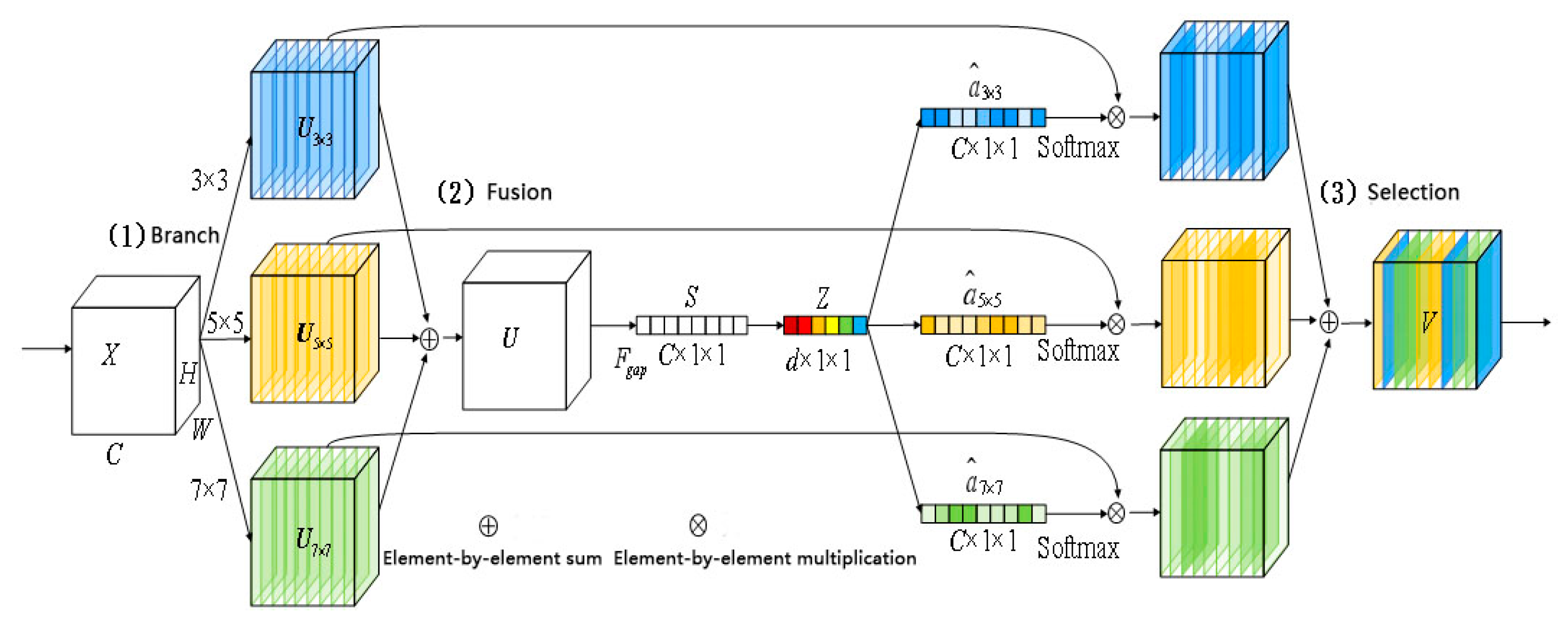Therefore, this paper introduces a dynamic selection mechanism of the convolution kernel [16], which allows convolutional layer neurons to adaptively select the size of their receptive field according to the input information. As shown in Figure 1, the dynamic selection mechanism of the convolution kernel includes three steps: branch, fusion and selection.

(1)

Branch: given input $X\in {ℝ}^{H\times W\times C}$, where H, W and C denote the height, width and channel of the input, respectively, perform three convolution conversions with convolution kernel sizes of 3 × 3, 5 × 5 and 7 × 7, $F_{3\times 3}:X\to U_{3\times 3}={ℝ}^{H\times W\times C}$,$F_{5\times 5}:X\to U_{5\times 5}={ℝ}^{H\times W\times C}$, $F_{7\times 7}:X\to U_{7\times 7}={ℝ}^{H\times W\times C}$.

(2)

Fusion: the convolution transformation results of the three branches are fused by element-by-element summation $U=U_{3\times 3}+U_{5\times 5}+U_{7\times 7}$. Then, apply global average pooling to compress the result of the fusion in the spatial dimension $H\times W$ to obtain global feature information $S=F_{\mathrm{gap}}\left(U\right)=\frac{1}{H\times W}{\displaystyle \sum _{i=1}^H{\displaystyle \sum _{j=1}^{W}U\left(i,j\right)}}$. Finally, through the fully connected layer, the global feature information $S\in {ℝ}^{1\times 1\times C}$ compressed as a feature $Z\in {ℝ}^{1\times 1\times d}$, the compression ratio is $r=C/d$. The purpose of compression is to enhance the nonlinear representation ability of the model.

(3)

Selection: use three fully connected layers to map the features $Z\in {ℝ}^{1\times 1\times d}$, and then three weight vectors $a_{3\times 3},b_{5\times 5}$ and $c_{7\times 7}$ are generated, respectively, where $a_{3\times 3},b_{5\times 5}, c_{7\times 7}\in {ℝ}^{1\times 1\times C}$. The weight vector is calculated by Softmax to obtain the result ${\widehat{a}}_{3\times 3},{\widehat{b}}_{5\times 5},{\widehat{c}}_{7\times 7}$, then add the vector ${\widehat{a}}_{3\times 3},{\widehat{b}}_{5\times 5},{\widehat{c}}_{7\times 7}$ to the feature matrix $U_{3\times 3},U_{5\times 5},U_{7\times 7}$ for weighted summation, generate the final output $V={\widehat{a}}_{3\times 3}\cdot U_{3\times 3}+{\widehat{b}}_{5\times 5}\cdot U_{5\times 5}+{\widehat{c}}_{7\times 7}\cdot U_{7\times 7}$. Thus, the importance of different branch information can be adjusted to realize the selection of a more suitable receptive field.

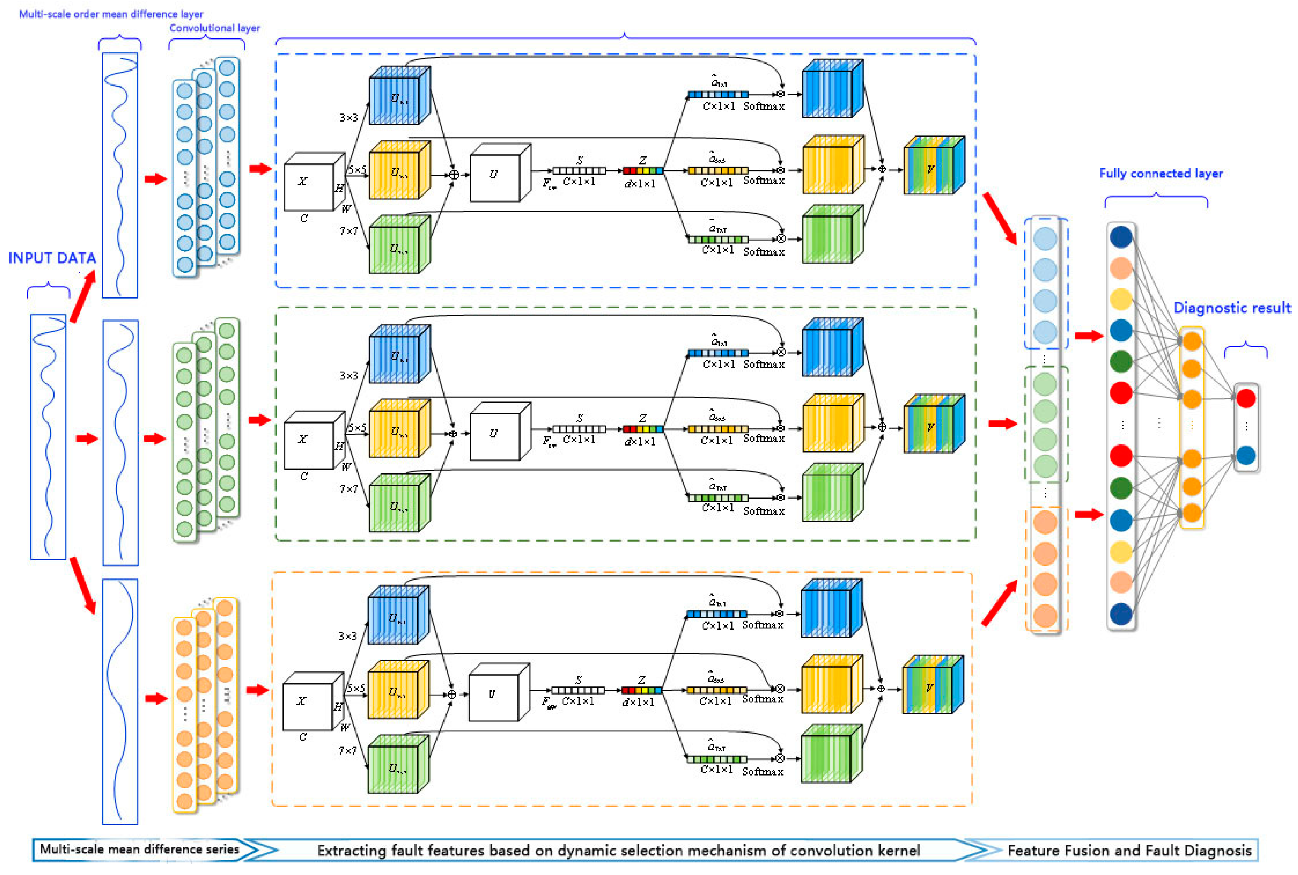
3.3. Mechanism MSCNN-SK Network

The MSCNN-SK (Multi-Scale Convolutional Neural Network with Selective kernel) network proposed in this paper is shown in Figure 2. It is mainly divided into a multi-scale mean difference layer, a feature extraction layer based on the dynamic selection mechanism of the convolution kernel, and a multi-scale information fusion layer.

The specific workflow of the MSCNN-SK network is described as follows: first, the multi-scale mean difference layer calculates the 0th order, 1st order and 2nd order mean difference sequences, and extracts the characteristics of the average rate of change of the time-domain response signal; secondly, the convolutional layer with the dynamic selection mechanism of the convolution kernel extracts fault characteristic information from the multi-scale mean difference data; then, the extracted multi-scale features are expanded into a one-dimensional vector and input to the two fully connected layers for information fusion and further feature extraction; finally, the fully connected layer obtains the analog circuit diagnosis results.

4. Case Studies Using the Proposed System

This section uses two representative circuits (Sallen–Key band-pass filter circuit and Four-opamp biquad high-pass filter circuit) to verify the effectiveness of the proposed method.

4.1. Data Collection

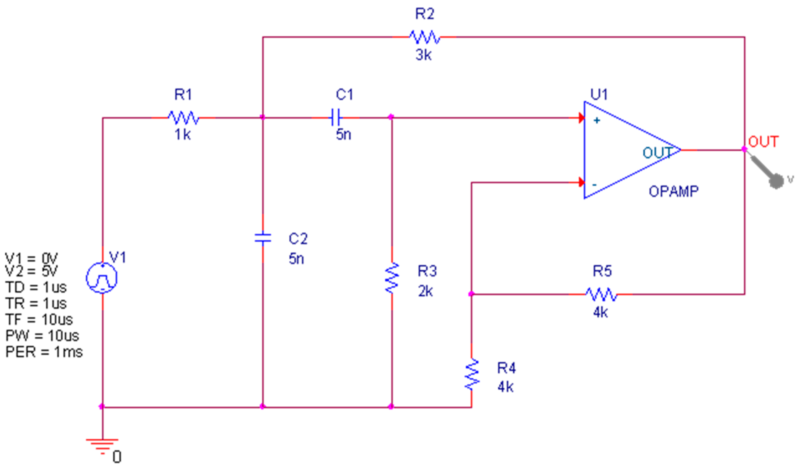
The principle of the Sallen–Key bandpass filter circuit is shown in Figure 3. This circuit includes 5 resistors, 2 capacitors and an operational amplifier. In the actual environment, the circuit component values fluctuate to a certain extent under the interference of environmental factors. Therefore, the tolerances of the resistors and capacitors in the circuit are set to 5% and 10%, respectively. In the circuit component sensitivity test, capacitors C1 and C2 and resistors R2 and R3 have a greater impact on the circuit, so these components are used as test components. The input of the circuit is a single pulse with a duration of 10 µs and an amplitude of 5 V, and the time domain response signal is collected at the output of the operational amplifier. The circuit has 9 modes, including No fault (NF) and 8 fault modes, namely C1 ↓, C1 ↑, C2 ↓, C2 ↑, R2 ↓, R2 ↑, R3 ↓ and R3 ↑. The symbols ↓ and ↑, respectively, indicate that the actual parameter value of the element is higher and lower than 50% of its nominal value.

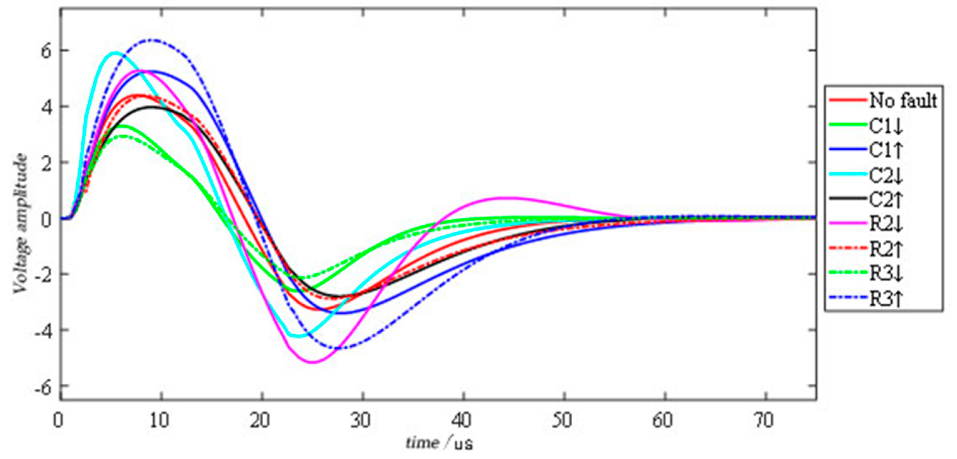
Figure 4 shows a set of time-domain response signals for each failure mode of the circuit under pulse input. It is easy to see from the figure that the difference in the time domain response signal is mainly in the first 75 µs. After that, the difference is negligible. Therefore, the sampling range of the original time domain response signal is set to 0–75 µs, the sampling interval is set to 0.5 µs, and 150 sampling points can be obtained for each time domain response signal. In this case, 2000 Monte Carlo analysis was performed for each failure mode; that is, there are 2000 samples for each failure mode. Shallen–key band-pass filter circuit fault code, fault mode, component nominal value and fault value are recorded in

Table 2. Failure mode of the Shallen–Key bandpass filter circuit.

Fault Code	Mode	Nominal Value	Tolerance Band	Fault Value
S0	No fault	-	-	-
S1	C1 ↓	5 nF	10%	2.5 nF
S2	C1 ↑	5 nF	10%	7.5 nF
S3	C2↓	5 nF	10%	2.5 nF
S4	C2 ↑	5 nF	10%	7.5 nF
S5	R2↓	3 kΩ	5%	1.5 kΩ
S6	R2 ↑	3 kΩ	5%	4.5 kΩ
S7	R3↓	2 kΩ	5%	1.0 kΩ
S8	R3 ↑	2 kΩ	5%	3.0 kΩ

.

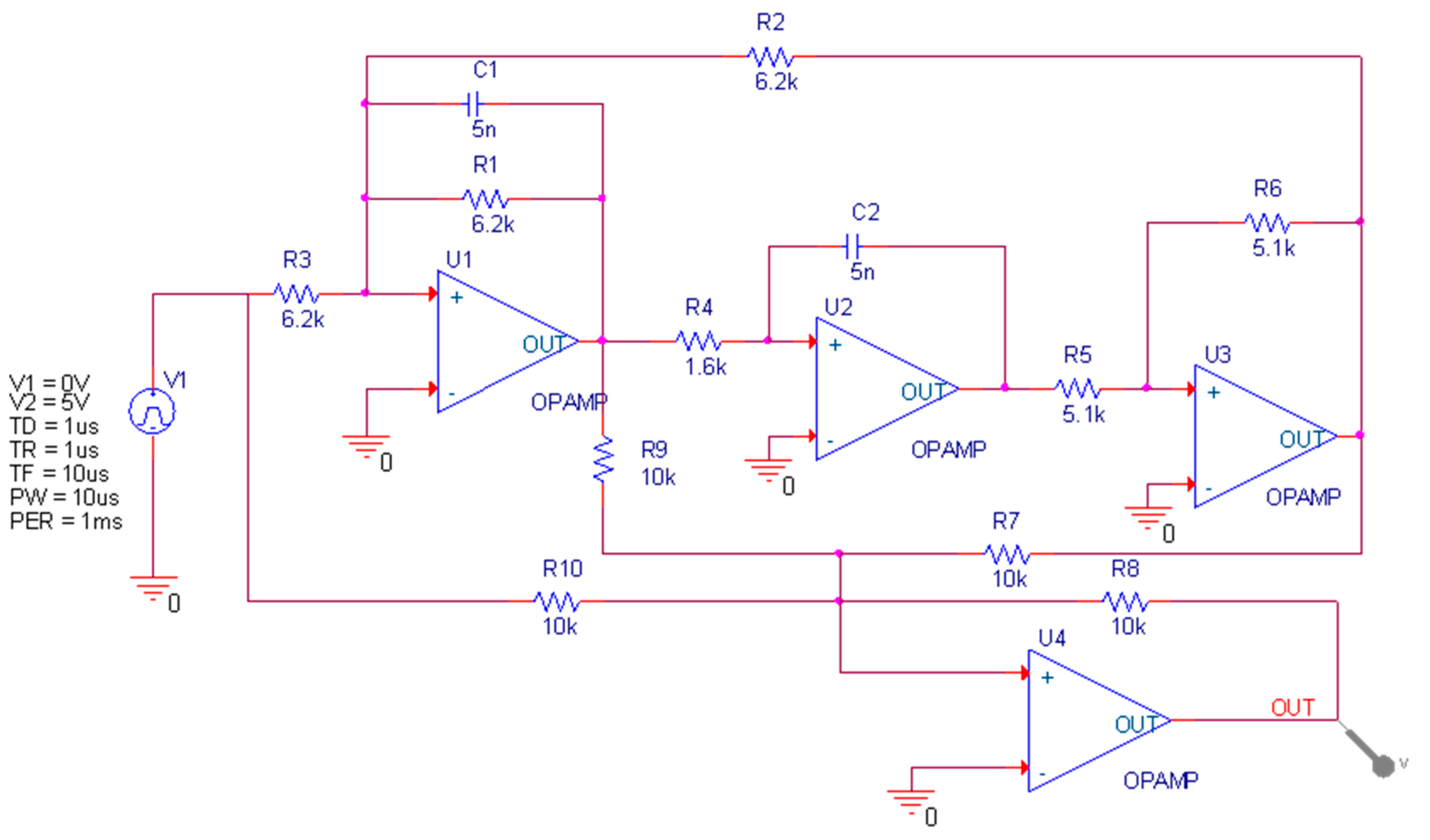
The Four-opamp double second-order high-pass filter circuit is shown in Figure 5. This circuit is composed of ten resistors, two capacitors and four operational amplifiers, which is more complex. As with the previous circuit, the tolerances of resistance and capacitance are 5% and 10%, respectively. The input of the circuit is a single pulse with a duration of 10 µs and an amplitude of 5 V. The time domain response signal is collected at the output of the operational amplifier U4. In the sensitivity test, capacitors C1 and C2 and resistors R1, R2, R3, and R4 have a greater impact on the circuit, so these components are used as test ones. Thirteen modes are set in the circuit, including No fault (NF) and 12 fault modes, namely C1 ↓, C1 ↑, C2 ↓, C2 ↑, R1 ↓, R1 ↑, R2 ↓, R2 ↑, R3 ↓, R3 ↑, R4 ↓ and R4 ↑. The symbol ↑ means that the actual parameter value of the component is higher than 50% of its nominal value; in the same way, ↓ means lower than 50% of its nominal value.

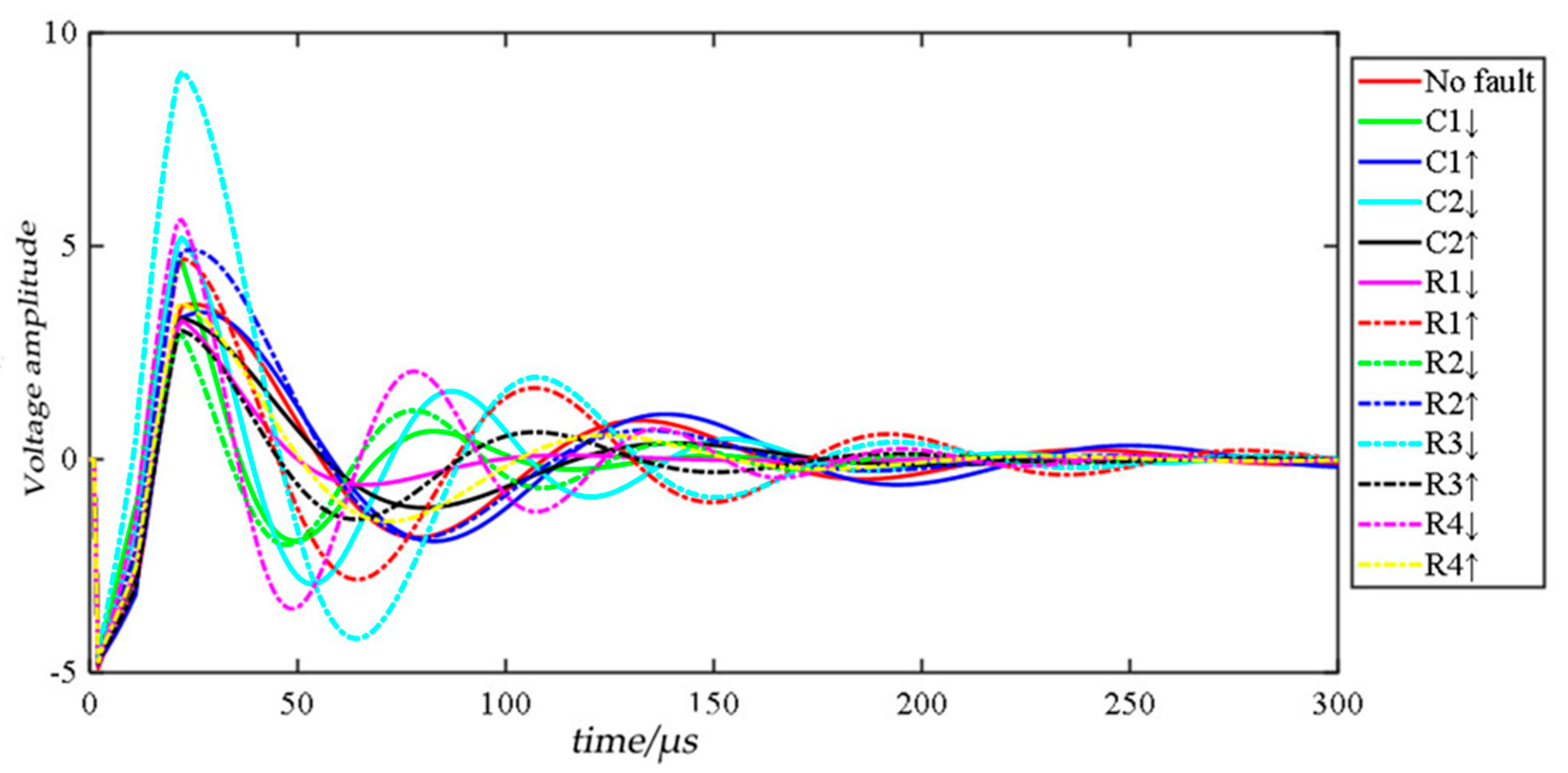
Figure 6 shows a set of time-domain response signals for each mode of the circuit under the pulse input of the operational amplifier U4. The signal is significantly different in the first 300 µs. Therefore, the sampling range of the time domain response signal is set to 0–300 µs, the sampling interval is 1 µs, and each time domain response signal generates a sample with 300 sampling points. In this circuit, 2000 Monte Carlo analyses are performed for each failure mode, and the entire data set has 13 failure modes, containing a total of 26,000 samples. The fault code, fault mode, component nominal value and fault value of the Four-opamp double second-order high-pass filter circuit are recorded in

Table 3. Failure mode of the Four-opamp biquad high-pass filter circuit.

Fault Code	Mode	Nominal Value	Tolerance Band	Fault Value
S0	No fault	-	-	-
S1	C1 ↓	5 nF	10%	2.5 nF
S2	C1 ↑	5 nF	10%	7.5 nF
S3	C2 ↓	5 nF	10%	2.5 nF
S4	C2 ↑	5 nF	10%	7.5 nF
S5	R1 ↓	6.2 kΩ	5%	3.1 kΩ
S6	R1 ↑	6.2 kΩ	5%	9.3 kΩ
S7	R2 ↓	6.2 kΩ	5%	3.1 kΩ
S8	R2 ↑	6.2 kΩ	5%	9.3 kΩ
S9	R3 ↓	6.2 kΩ	5%	3.1 kΩ
S10	R3 ↑	6.2 kΩ	5%	9.3 kΩ
S11	R4 ↓	1.6 kΩ	5%	0.8 kΩ
S12	R4 ↑	1.6 kΩ	5%	2.4 kΩ

.

4.2. Experimental Comparison and Result Analysis

In order to verify the effectiveness of the proposed MSCNN-SK network, this section conducts fault diagnosis comparative experiments based on the data sets simulated by the two benchmark test circuits built earlier. In the experiment, four typical DL networks were used for comparison, namely: Recurrent Neural Network (RNN), Long Short-Term Memory (LSTM) and Back Propagation Neural Network (BPNN). The RNN and LSTM network consists of two hidden layers, with 128 hidden units. The BPNN network has 3 hidden layers. The 1DCNN network includes 3 layers of convolutional layers, 3 layers of pooling layers, and the size and number of convolution kernels are set to 1 × 3 and 32, respectively. The MSCNN-SK network has three branches corresponding to the 0th order, 1st order, and 2nd order mean difference sequences, and the network structure of each branch is the same. Note that we determine the parameters of the network according to popular recommendations [20,21] as well as trial and error.

Take the first branch as an example, the parameters of the convolutional layer and pooling layer of the initial part of the network are 1 × 1 × 32 and 1 × 5, respectively. In the convolution module based on the dynamic selection mechanism of the convolution kernel, the three convolution layer parameters are 1 × 3 × 32, 1 × 5 × 32, and 1 × 7 × 32, that is, the size of the convolution kernel is 1 × 3, 1 × 5 and 1 × 7, and the compression ratio is set to 16. In addition, all test models are independently tested 10 times to reduce the influence of random errors. All the DL networks are implemented by the Pytorch library. During the network training phase, the cross-entropy function is adopted as the loss function, and the Adam optimizer is used with a learning rate fixed to 0.001 and a batch size of 64. It should be mentioned that all the hyper parameters are determined by trial and error.

The size of the Shalley-Key Bandpass Filter fault diagnosis dataset is 18,000 × 150, and the input size of each network is 1 × 150. A total of 70% of the data are taken as the training set while the other 30% data are used as the testing set.

Table 4. Shallen–Key band-pass filter circuit fault diagnosis comparative experiment.

Norm	BPNN	RNN	LSTM	1DCNN	MSCNN-SK
Maximum	100.00	99.91	100.00	100.00	100.00
Minimum	99.98	99.85	99.87	100.00	100.00
Average	99.99	99.87	99.93	100.00	100.00
SD	0.01	0.02	0.06	0.00	0.00

lists the maximum, minimum, average and standard deviation results of all test networks in the Sallen–Key band-pass filter circuit fault diagnosis. As shown in Table 4, the average fault diagnosis accuracy rate of 1DCNN and MSCNN-SK networks has reached 100%, while the average fault diagnosis accuracy rate of BPNN, RNN and LSTM networks is also close to 100%. As mentioned above, the Sallen–Key bandpass filter circuit has fewer components and a relatively simple structure. The tested deep learning methods can achieve high diagnostic accuracy.

As aforementioned, the Four-opamp double second-order high-pass filter circuit fault diagnosis dataset has 26,000 samples, and each sample size, i.e., the input size of each network, is 1 × 300. We also take 70% of data as the training set and the test data as the testing set.

Table 5. Four-opamp double second-order high-pass filter circuit fault diagnosis comparative experiment.

Norm	BPNN	RNN	LSTM	1DCNN	MSCNN-SK
Maximum	99.15	96.46	99.21	99.09	99.92
Minimum	98.91	88.17	98.95	98.95	99.80
Average	99.04	92.13	99.09	99.03	99.87
SD	0.08	2.03	0.08	0.04	0.03

shows the comparison results of Four-opamp double second-order high-pass filter circuit fault diagnosis. It is easy to see from the table that the average fault diagnosis accuracy of the RNN network is 92.13%, which is much lower than the other four models. This is because the RNN network is prone to gradient dispersion and gradient explosion. The average fault diagnosis results obtained by BPNN, LSTM and 1DCNN are close to about 99%, while the performance of the LSTM network is slightly better than that of the BPNN and 1DCNN networks. The diagnostic accuracy achieved by MSCNN-SK is higher than the other four network models, reaching 99.87%. At the same time, the standard deviation is also the smallest among the five test methods. This shows that the MSCNN-SK network can effectively extract the essential characteristics of the fault. A good fault diagnosis effect can also be achieved in complex circuit fault diagnosis.

4.3. Feature Visualization Analysis

The t-SNE technology is a non-linear unsupervised dimensionality reduction method commonly used in the field of deep learning. This method can visualize high-dimensional features in a two-dimensional space to intuitively judge whether the high-dimensional features are discriminative [17,18]. This section uses t-SNE technology to visualize the original fault data of the two benchmark test circuits and the high-dimensional features extracted from the last layer of the BPNN, RNN, LSTM, 1DCNN and MSCNN-SK models in two dimensions.

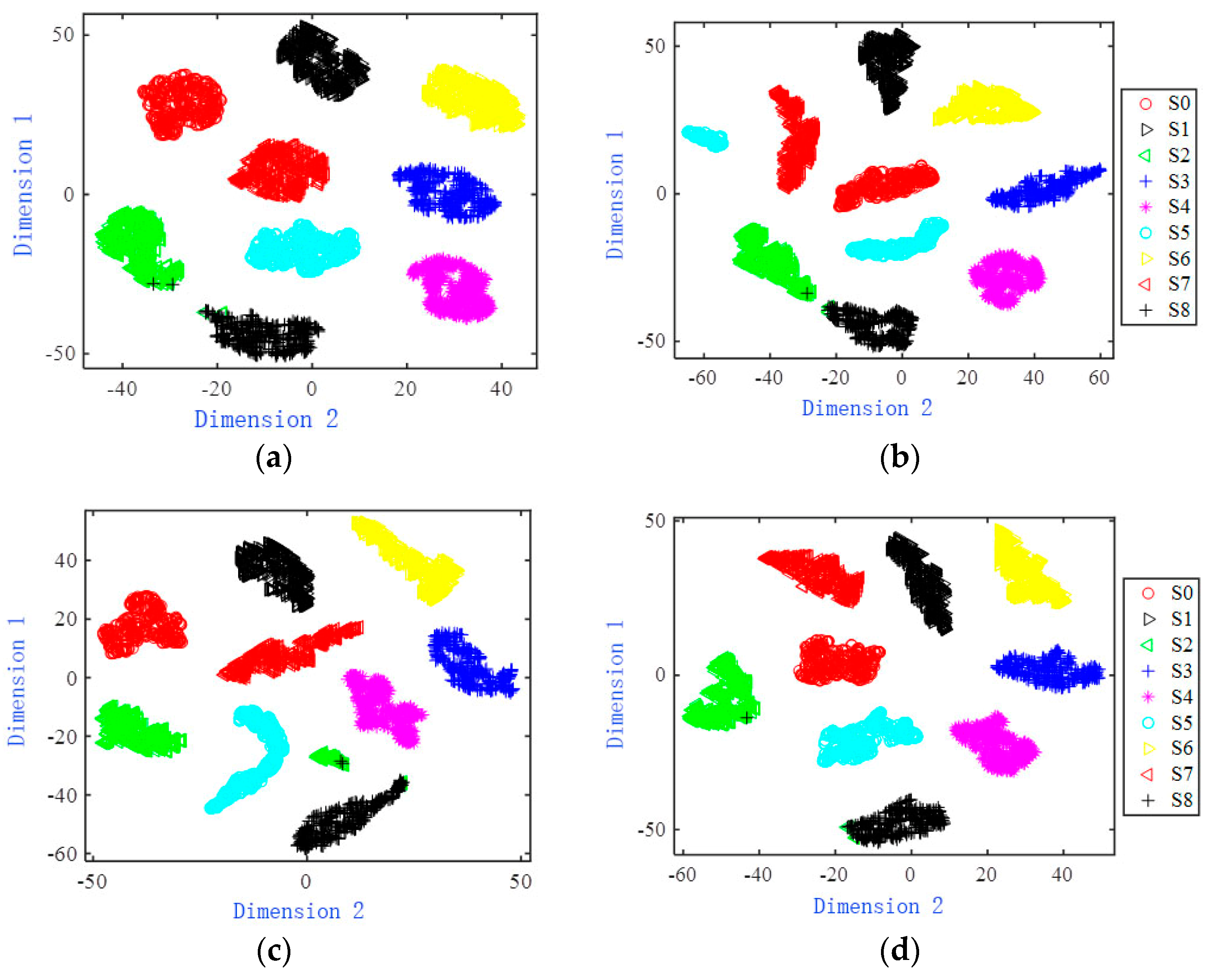
The original data of the Sallen–Key band-pass filter circuit and the features extracted from each model are visualized in two dimensions and shown in Figure 7. From Figure 7a–d, in the two-dimensional scattered point distribution of the original fault data and the features extracted by networks such as BPNN, RNN and LSTM, there are a small number of overlapping sample points in the fault modes S2 and S8, and the remaining fault mode sample points are completely separated. Figure 7e,f, respectively show the two-dimensional visualization results of the features extracted by the 1DCNN and MSCNN-SK networks. It can be clearly seen from the figure that the sample points of each failure mode have been completely separated, and the two-dimensional scattered points have independent distribution areas. In addition, the two-dimensional scattered points of each failure mode in Figure 7f are more closely distributed.

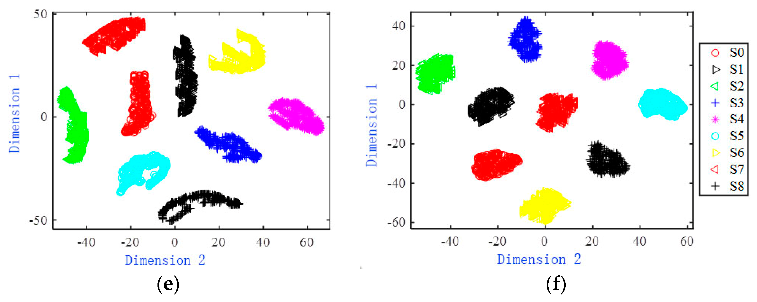
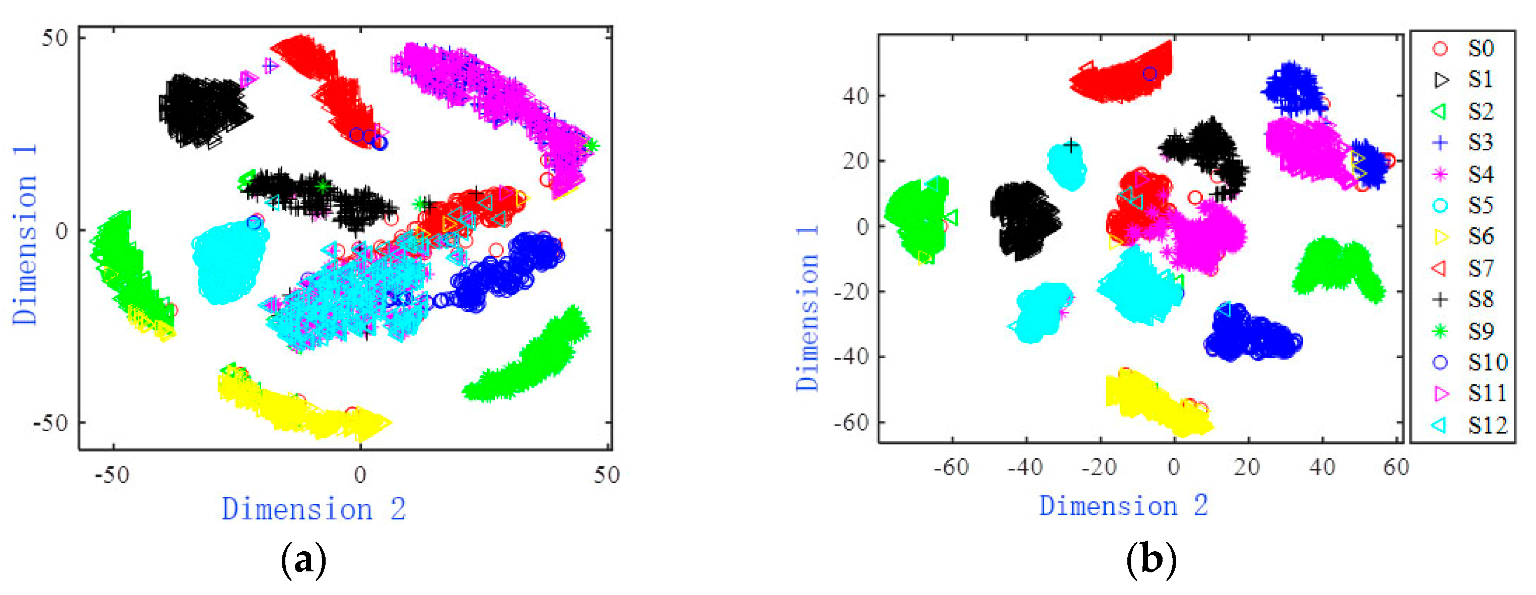
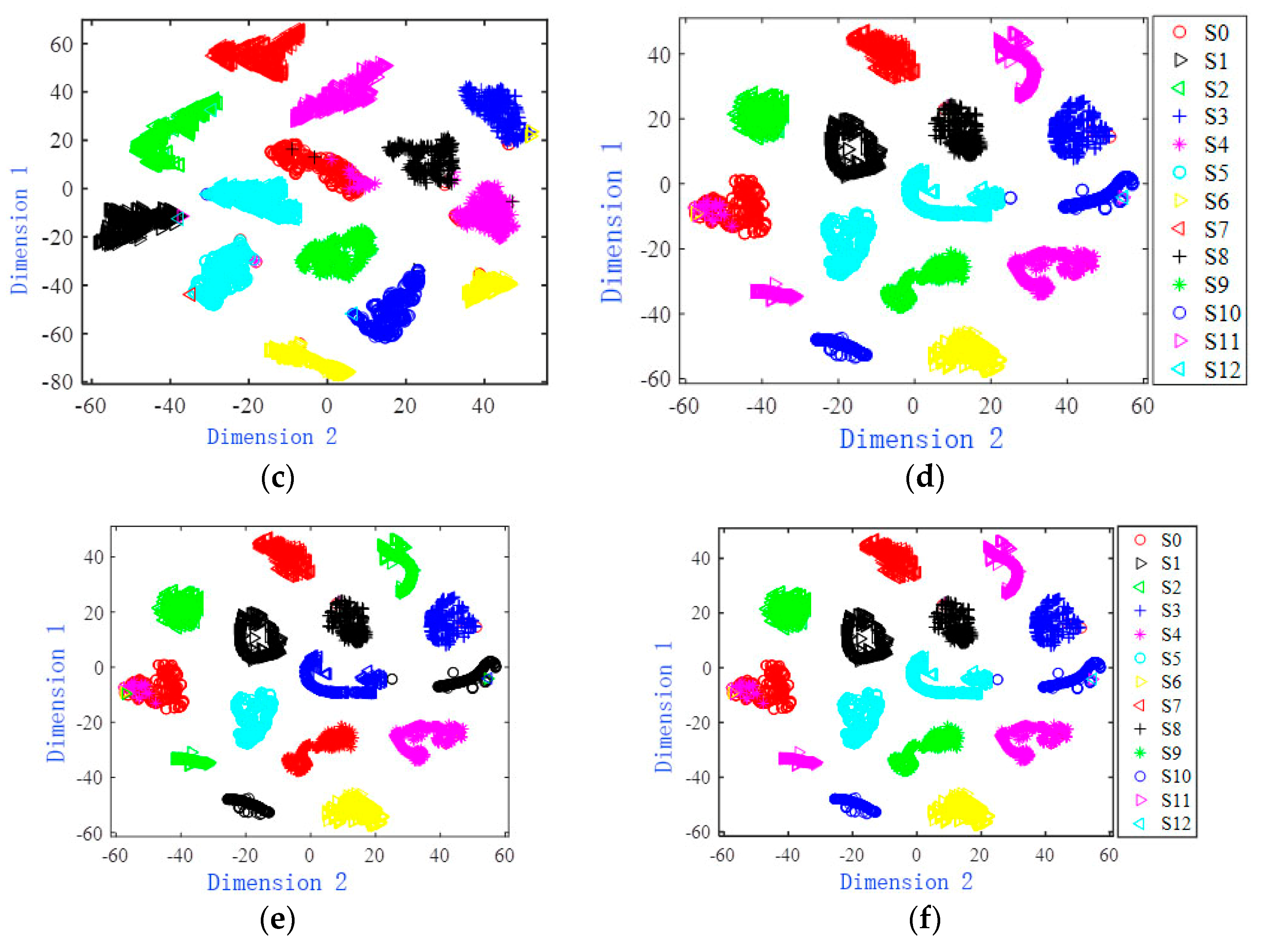
The original and characteristic two-dimensional visualization effect of the Four-opamp biquad high-pass filter is shown in Figure 8. It can be seen from Figure 8a that the sample distribution of each failure mode of the original data is relatively close, and there is a large amount of overlap. Figure 8b,c are two-dimensional scatter plots of the features extracted by the BPNN network and the RNN network. There are still some overlapping sample points in some failure modes in the figure. The two-dimensional scatter diagram of features extracted from LSTM network and CNN network is shown in Figure 8d,e. Most two-dimensional scatter points of fault modes have been completely separated, and the number of overlapping sample points is relatively small, but the distribution range of most fault mode samples is relatively scattered. Figure 8f draws a scatter diagram of the features extracted by the MSCNN-SK network. It can be seen that the two-dimensional scatter points of the same failure mode are concentrated, and there are almost no overlapping sample points, which is easy to distinguish.

Based on the two-dimensional visualization comparison results of Figure 7 and Figure 8, it can be concluded that the MSCNN-SK network proposed in this paper can effectively extract the deep fault features of analog circuits. The extracted features have a high degree of discrimination and concentrated distribution, which is beneficial to further fault classification.

5. Conclusions

Aiming at the problem that the 1DCNN network performs poorly in the fault diagnosis of complex analog circuits, this paper proposes the MSCNN-SK network. On the basis of the 1DCNN network, this network adds a multi-scale average deviation layer to calculate the 0th-order, 1st-order and 2nd-order average deviation sequences, extracts the average rate of change characteristics of the circuit’s time domain response signal, and introduces the dynamic convolution kernel selection mechanism that enables the network to adaptively select a suitable size convolution kernel during the feature extraction process without manual intervention.

Through the simulation experiments of two benchmark test circuits, the fault diagnosis comparison experiment was first carried out. Networks such as BPNN, RNN, LSTM and 1DCNN were selected as the comparison methods. The results show that the MSCNN-SK network can identify the fault of the Shallen–Key band-pass filter circuit 100%. In the more complex Four-opamp double second-order high-pass filter circuit, the average fault diagnosis accuracy rate has reached 99.87%. At the same time, after using t-SNE technology to visualize the features extracted by each model in two dimensions, the features extracted by the MSCNN-SK network have the highest separation. In the two-dimensional visual comparison of the features extracted by each model, the features extracted by the MSCNN-SK network are also the most discriminative.

The proposed MSCNN-SK network can be directly used for other fault classification cases. In future work, we will apply the proposed MSCNN-SK network to more analog circuit fault diagnosis to further evaluate its generalization ability.

References

- Gao, T.; Yang, J.; Jiang, S. A novel incipient fault diagnosis method for analog circuits based on GMKL-SVM and wavelet fusion features. IEEE Trans. Instrum. Meas. 2020, 70, 3502315. [Google Scholar] [CrossRef]
- He, W.; He, Y.; Li, B. Generative adversarial networks with comprehensive wavelet feature for fault diagnosis of analog circuits. IEEE Trans. Instrum. Meas. 2020, 69, 6640–6650. [Google Scholar] [CrossRef]
- Aminian, M.; Aminian, F. Neural-network based analog-circuit fault diagnosis using wavelet transform as preprocessor. IEEE Trans. Circuits Syst. II Analog. Digit. Signal Processing 2000, 47, 151–156. [Google Scholar] [CrossRef]
- Cui, Y.; Shi, J.; Wang, Z. Analog circuit fault diagnosis based on quantum clustering based multi-valued quantum fuzzification decision tree (QC-MQFDT). Measurement 2016, 93, 421–434. [Google Scholar] [CrossRef]
- Aminian, F.; Aminian, M. Fault diagnosis of analog circuits using Bayesian neural networks with wavelet transform as preprocessor. J. Electron. Test. 2001, 17, 29–36. [Google Scholar] [CrossRef]
- Ma, Q.; He, Y.; Zhou, F. A new decision tree approach of support vector machine for analog circuit fault diagnosis. Analog. Integr. Circuits Signal Processing 2016, 88, 455–463. [Google Scholar] [CrossRef]
- Zhang, C.; He, Y.; Yuan, L.; He, W.; Xiang, S.; Li, Z. A novel approach for diagnosis of analog circuit fault by using GMKL-SVM and PSO. J. Electron. Test. 2016, 32, 531–540. [Google Scholar] [CrossRef]
- Yuan, L.; He, Y.; Huang, J.; Sun, Y. A new neural-network-based fault diagnosis approach for analog circuits by using kurtosis and entropy as a preprocessor. IEEE Trans. Instrum. Meas. 2009, 59, 586–595. [Google Scholar] [CrossRef]
- Passricha, V.; Aggarwal, R.K. A hybrid of deep CNN and bidirectional LSTM for automatic speech recognition. J. Intell. Syst. 2020, 29, 1261–1274. [Google Scholar] [CrossRef]
- Vlachostergiou, A.; Caridakis, G.; Mylonas, P.; Stafylopatis, A. Learning Representations of Natural Language Texts with Generative Adversarial Networks at Document, Sentence, and Aspect Level. Algorithms 2018, 11, 164. [Google Scholar] [CrossRef] [Green Version]
- Kasper-Eulaers, M.; Hahn, N.; Berger, S.; Sebulonsen, T.; Myrland, Ø.; Kummervold, P.E. Short Communication: Detecting Heavy Goods Vehicles in Rest Areas in Winter Conditions Using YOLOv5. Algorithms 2021, 14, 114. [Google Scholar] [CrossRef]
- Su, X.; Cao, C.; Zeng, X.; Feng, Z.; Shen, J.; Yan, X.; Wu, Z. Application of DBN and GWO-SVM in analog circuit fault diagnosis. Sci. Rep. 2021, 11, 7969. [Google Scholar] [CrossRef] [PubMed]
- Zhao, G.; Liu, X.; Zhang, B.; Liu, Y.; Niu, G.; Hu, C. A novel approach for analog circuit fault diagnosis based on deep belief network. Measurement 2018, 121, 170–178. [Google Scholar] [CrossRef]
- Wang, H.; Liu, Z.; Peng, D.; Qin, Y. Understanding and learning discriminant features based on multiattention 1DCNN for wheelset bearing fault diagnosis. IEEE Trans. Ind. Inform. 2019, 16, 5735–5745. [Google Scholar] [CrossRef]
- Ji, L.; Fu, C.; Sun, W. Soft Fault Diagnosis of Analog Circuits Based on a ResNet With Circuit Spectrum Map. IEEE Trans. Circuits Syst. I Regul. Pap. 2021, 68, 2841–2849. [Google Scholar] [CrossRef]
- Yang, H.; Meng, C.; Wang, C. Data-driven feature extraction for analog circuit fault diagnosis using 1-D convolutional neural network. IEEE Access 2020, 8, 18305–18315. [Google Scholar] [CrossRef]
- Du, T.; Zhang, H.; Wang, L. Analogue circuit fault diagnosis based on convolution neural network. Electron. Lett. 2019, 55, 1277–1279. [Google Scholar] [CrossRef]
- Ioffe, S.; Szegedy, C. Batch normalization: Accelerating deep network training by reducing internal covariate shift. In Proceedings of the International Conference on Machine Learning, PMLR, Lille, France, 6–11 July 2015; pp. 448–456. [Google Scholar]
- Glorot, X.; Bengio, Y. Understanding the difficulty of training deep feedforward neural networks. J. Mach. Learn. Res. 2010, 9, 249–256. [Google Scholar]
- Hao, S.; Ge, F.X.; Li, Y.; Jiang, J. Multisensor bearing fault diagnosis based on one-dimensional convolutional long short-term memory networks. Measurement 2020, 159, 107802. [Google Scholar] [CrossRef]
- Shi, J.; Peng, D.; Peng, Z.; Zhang, Z.; Goebel, K.; Wu, D. Planetary gearbox fault diagnosis using bidirectional-convolutional LSTM networks. Mech. Syst. Signal Processing 2022, 162, 107996. [Google Scholar] [CrossRef]