Efficient Construction of the Equation Automaton

Abstract

This paper describes a fast algorithm for constructing directly the equation automaton from the well-known Thompson automaton associated with a regular expression. Allauzen and Mohri have presented a unified construction of small automata and gave a construction of the equation automaton with time and space complexity in $O(mlogm+m^2)$, where m denotes the number of Thompson automaton transitions. It is based on two classical automata operations, namely epsilon-removal and Hopcroft’s algorithm for deterministic Finite Automata (DFA) minimization. Using the notion of c-continuation, Ziadi et al. presented a fast computation of the equation automaton in $O(m^2)$ time complexity. In this paper, we design an output-sensitive algorithm combining advantages of the previous algorithms and show that its computational complexity can be reduced to $O(m\times |Q_{{\equiv }_e}|)$, where $|Q_{{\equiv }_e}|$ denotes the number of states of the equation automaton, by an epsilon-removal and Bubenzer minimization algorithm of an Acyclic Deterministic Finite Automata (ADFA).

1. Introduction

The equation automaton (also known as derived terms automaton or Antimirov automaton) was first introduced in Mirkin’s paper [1]. In [2], Antimirov introduced the notion of partial derivative of a regular expression, that lead to another definition and construction of the equation automaton. It is an $ϵ$-free NFA which has in general smaller number of states and transitions than the well-known position automaton [3,4,5]. The complexity of the original construction algorithm of [2], which is based on the computation of the set of partial derivatives of the expression, is in $O(n^5)$, where n denotes the size of the regular expression. In 2001, Champarnaud and Ziadi [6] introduced the notion of canonical derivatives and constructed a new automaton called the c-continuation automaton. They also proved that this automaton is isomorphic to the position automaton and that the equation automaton is its quotient for some equivalence relation.

The notion of c-derivative has been introduced in [6] to derive the equation automaton from the position automaton via the c-continuation automaton. A unique regular expression over indexed and ordered letters, called c-continuation, is assigned to each state of the position automaton. The resulting automaton is called the c-continuation automaton [6]. After that, one can define the equivalence relation between two c-continuations i.e., two states of the c-continuation automaton as follows: if deleting the indices of letters from two c-continuations results in the same regular expression, they correspond to the same partial derivative. Hence, the equation automaton would be a quotient of the c-continuation automaton w.r.t. the previously defined equivalence relation. From the algorithmic point of view, this result allows the construction of the equation automaton in $O(n^2)$ time and space [6,7]. Therefore, this improves the Antimirov’s algorithm by a factor of $O(n^3)$.

In [8], Allauzen and Mohri present simple and unified constructions of the position automata [3,4,5], follow automata [9,10], and the equation automata [2,6,7] from regular expressions. Their algorithms are based on two standard automata operations applied to the Thompson automata [11,12] called: epsilon-remove and Hopcroft’s algorithm for DFA minimization [13]. The complexity of their construction for the equation automaton is in $O(mlogm+m^2)$, where m is the number of Thompson automaton transitions. Notice that, by construction the number of transitions of the Thompson automaton m and the size of a regular expression n are proportional. Thus, we have $m=O(n)$.

To improve the time complexity of computing the equation automaton from a regular expression E, we design an algorithm, combining advantages of previous methods [6,7,8], with a worst-case time complexity in $O(m\times |Q_{{\equiv }_e}|)$, where $|Q_{{\equiv }_e}|$ denotes the number of its states. Our approach is based on Bubenzer minimization of an acyclic DFA instead Hopcroft’s algorithm for DFA minimization step used in Allauzen and Mohri’s method. The main idea is to associate implicitly each c-continuation to a corresponding state, called position state in the Thompson automaton by a special marking of $\epsilon$-transitions. As a consequence of this marking, the right language of each position state in the Thompson automaton represents implicitly its c-continuation, called pseudo-continuation. After that, we disable temporarily the cyclic $\epsilon$-transition in the Thompson automaton and perform Bubenzer minimization of an acyclic DFA to compute efficiently partial derivatives equivalence relation over the set of position states. Finally, we remove indexed $\epsilon$-transitions, enable the cyclic $\epsilon$-transition and then compute the $\epsilon$-closure of states in the produced automaton from the previous step to get the equation automaton. The implementation of the proposed algorithm is available under the repository https://github.com/FaissalOuardi/Equation-automaton, (accessed on 27 May 2021).

The paper is organized as follows. Section 2 contains some basic definitions and necessary preliminaries. Section 3 summarizes theoretical results that lead to c-continuations of a regular expression, and their relations with the partial derivatives. The definition of the c-continuation automaton is recalled, as well as the way it is connected to the equation automaton. Section 4 is a recall to the algorithm due to Allauzen and Mohri. We detail then in Section 5 the algorithmic refinements leading to an $O(m\times |Q_{{\equiv }_e}|)$ time complexity of the efficient construction of the equation automaton where $|Q_{{\equiv }_e}|$ is the number of its states.

2. Preliminaries

In this section, we introduce briefly the notion of finite automata. For further details on formal aspects of finite automata theory, we particularly recommend reading classical books [14,15].

2.1. Regular Expressions and Finite Automata

Let A be a non-empty finite set of letters, called an alphabet. The set of all words over A is denoted by $A^{\ast }$. $\epsilon$ is the empty word. A language over A is a subset of $A^{\ast }$.

2.1.1. Regular Expressions and Languages

A regular expression over the alphabet A is a term of the algebra ${\mathcal{T}}_{reg(A)}$ defined over the set $A\cup \{0,1\}$ with the symbols of functions $\ast ,+,·,$ where ∗ is unary and + and · are binary. Properties of the constants $0,1$ and the operators $\ast ,+$, and · lead to identities on this algebra. Each regular expression denotes a language. L is the function that assigns to each regular expression the regular language it denotes. $L:T_{reg(A)}⟶reg(A^{\ast })$ is defined as follows:

$$\begin{array}{ccc}\hfill L(0)& =& \varnothing \hfill \\ \hfill L(1)& =& \{\epsilon \}\hfill \\ \hfill L(a)& =& a,\mathrm{for} \mathrm{each}a\mathrm{in}A\hfill \\ \hfill L(F+G)& =& L(F)\cup L(G)\hfill \\ \hfill L(F·G)& =& L(F)L(G)\hfill \\ \hfill L(F^{\ast })& =& L{(F)}^{\ast }\hfill \end{array}$$

The following identities are classically used:

$$\begin{array}{c}\hfill 0+E=E=E+0,1·E=E=E·1,0·E=0=E·0.\end{array}$$

Let E be a regular expression. The set of letters occurring in E is denoted by $A_E$. To specify their position in the expression, letters are subscripted following the order of reading. The resulted expression is the linearized form of E, denoted by $\overline{E}$. For example, starting from $E={(a+b)}^{\ast }aba+1$, one obtains the linearized version $\overline{E}={(a_1+b_2)}^{\ast }{a}_3{b}_4{a}_5+1$ of E. The subscripted letters are called positions; the set of all position in the expression E is denoted by $pos(E)$. For the previous example, we have $pos(E)=\{a_1,b_2,a_3,b_4,a_5\}$. If F is a subexpression of E, we denote by ${pos}_E(F)$ the subset of positions of E that are letters of F. We say that a regular expression is in linear form if each letter of the expression occurs only once. We denote by h the function that maps each position in $pos(E)$ to the letter of $A_E$ that appears at this position in E. For $E={(a+b)}^{\ast }aba+1$, we have $h(a_1)=h(a_3)=h(a_5)=a$ and $h(b_2)=h(b_4)=b$. The size of the regular expression E, denoted by $|E|$, is the number of nodes in its syntax tree. We call alphabetic width of E, denoted by $||E||$, the number of occurrences of letters in the expression i.e., the cardinality of $pos(E)$. The alphabetic width of the expression ${(a+b)}^{\ast }aba+1$ is equal to 5; its size is equal to 12.

Notice that the alphabetic width and the size of a regular expression are independent parameters. Therefore complexities are expressed w.r.t. both of these two parameters. However, it is usual to preprocess the input expression in order to reduce its size and to make its size proportional to its alphabetic width. So, if we consider a reduced regular expression E w.r.t. the following rules:

• $1+1=1$,
• $1+E+1=1+E$,
• E is in Star-Normal Form (SNF) [16].

Thus, we have in this case $|E|=O(||E||)$. It is known that regular expressions can be transformed to SNF in linear time [16]. $\lambda (E)$ denote the null term of E, that is

$$\lambda (E)=\left\{\begin{array}{cc}1\hfill & \mathrm{if} \epsilon \in L(E),\hfill \\ 0\hfill & \mathrm{otherwise}.\hfill \end{array}\right.$$

By $T(E)$ we denote the syntax tree associated with the regular expression E. A node in $T(E)$ will be denoted by $\nu$. We write $\mathit{Nodes}(E)$ for the set of nodes of $T(E)$. If $\nu \in \mathit{Nodes}(E)$ is a node in $T(E),\mathit{sym}(\nu ),\mathit{father}(\nu )$ and $\mathit{right}(\nu )$ denote respectively the symbol, the father and the right son of the node $\nu$. If $\mathit{sym}(\nu )$ is an operator, $E_{\nu }$ will denote the subexpression that corresponds to the subtree with the root $\nu$.

2.1.2. Finite Automata and Recognizable Languages

A nondeterministic finite automaton (NFA) is a quintuple $\mathcal{A}=⟨Q,A,q_0,\delta ,F⟩$ where Q is a finite set of states, A is the alphabet, $q_0\in Q$ is the initial state, $F\subseteq Q$ is the set of final states, and $\delta :Q\times (A\cup \{\epsilon \})\to 2^Q$ is the transition function. The size of an automaton $\mathcal{A}$, denoted by $|\mathcal{A}|$, is the number of its states. The automaton $\mathcal{A}$ is called deterministic (DFA) if there is only one initial state, $|\delta (q,\epsilon )|=0$ and $|\delta (q,a)|=1$, for any $q\in Q$, for any $a\in A$. A path in $\mathcal{A}$ is a sequence $(q_i,a_i,q_{i+1}),i=1,\cdots ,n$, of consecutive transitions. Its label is the word $w=a_1{a}_2\cdots a_n$. A word $w=a_1{a}_2\cdots a_n$ is recognized by the automaton $\mathcal{A}$ if there exists a path labeled w such that $q_1=q_0$ and $q_{n+1}\in F$.

The language recognized by the automaton $\mathcal{A}$, denoted by $L(\mathcal{A})$, is the set of words it recognizes. The right language of a state q in the automaton $\mathcal{A}$, denoted by ${\overrightarrow{L}}_q(\mathcal{A})$, is obtained by setting q to be the initial state, i.e., ${\overrightarrow{L}}_q(\mathcal{A})=\{w\in A^{\ast }|\delta (q,w)\cap F\ne \varnothing \}$.

We say that $\mathcal{A}$ is acyclic if the underlying graph is acyclic. The language associated with an acyclic automaton is finite.

Let ∼ be an equivalence relation over Q. For $q\in Q$, $[q]$ denotes the equivalence class of q w.r.t. ∼ and, for $C\subseteq Q,C{/}_{\sim }$ denotes the quotient set $C{/}_{\sim }=\{[q]|q\in C\}$. We say that ∼ is right invariant w.r.t. $\mathcal{A}$ if and only if the following conditions hold:

• $\sim \subseteq {(Q-F)}^2\cup F^2$ (final and non-final states are not ∼-equivalent),
• for any $p,q\in Q$, $a\in A$, if $p\sim q$, then $\delta (p,a){/}_{\sim }=\delta (q,a){/}_{\sim }$.

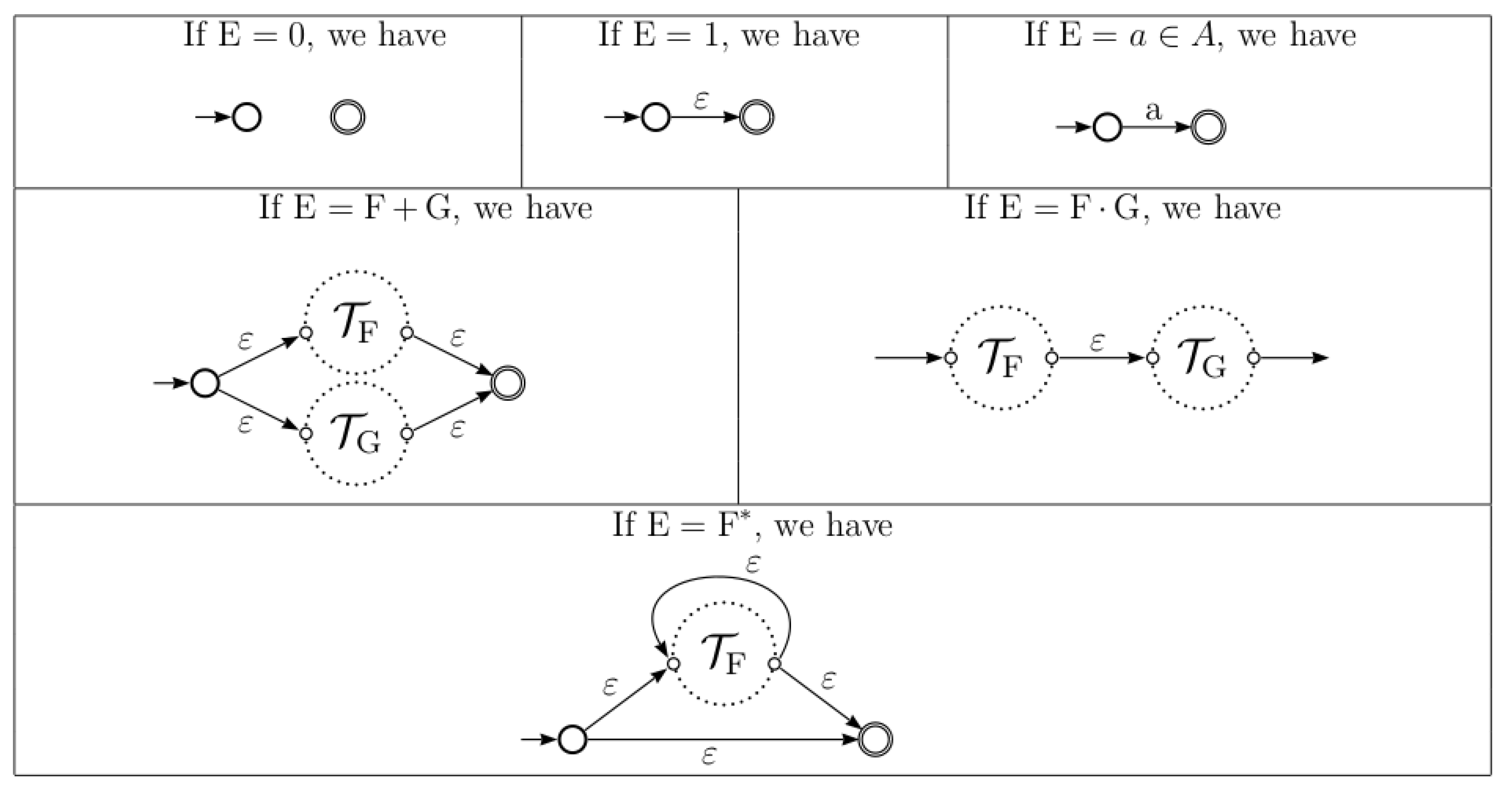
2.2. Thompson Automaton

In [12], Thompson gave a linear time and space algorithm to convert a regular expression E to an NFA with $\epsilon$-transitions, denoted by ${\mathcal{T}}_E$. The recursive steps of the construction of Thompson NFA are pictured in Figure 1.

Example 1.

Let us consider the regular expression $E={(a^{\ast }+b{a}^{\ast }+b^{\ast })}^{\ast }$. The Thompson automaton ${\mathcal{T}}_E$ associated with E is shown in the Figure 2.

Figure 2. Thompson automaton ${\mathcal{T}}_E$.

Figure 1. Thompson construction of an NFA.

There are some disadvantages of Thompson’s NFA when it is used in practice: it has many redundant states and $\epsilon$-transitions, its number of states is in $O(|E|)$ while other constructions offer NFAs with $O(||E||)$ states.

In the next section, we will present the construction of a reduced $\epsilon$-free automaton, named equation automaton, sometimes called Antimirov automaton or derived terms automaton.

3. Equation Automaton

The equation automaton has been introduced for the first time by Mirkin in [1]. In 1996, Antimirov introduced the notion of partial derivatives and used it to define the equation automaton [2]. Champarnaud and Ziadi [6] defined the notion of canonical derivatives of a linear expression and constructed a new automaton called the c-continuation automaton. They also proved that this automaton is isomorphic to the position automaton in the sense that the two automata have identical sets of states, identical initial and final states, and transitions Theorem 6 in [6]. Using an equivalence relation over the set of states of the c-continuation automaton, they derive the equation automaton in quadratic time.

The definition of the equation automaton of a regular expression is based on that of the partial derivatives of regular expressions, which are multisets of regular expressions over A. The partial derivative of E with respect to $a\in A$ is defined recursively on the structure of E as follows:

$$\begin{array}{ccc}\hfill {\partial }_a(0)& =& {\partial }_a(1)=\varnothing ,\hfill \\ \hfill {\partial }_a(x)& =& \mathbf{if}a=x\mathbf{then}\{1\}\mathbf{else}\varnothing ,\hfill \\ \hfill {\partial }_a(F+G)& =& {\partial }_a(F)\cup {\partial }_a(G),\hfill \\ \hfill {\partial }_a(F·G)& =& {\partial }_a(F)·G\cup \lambda (F)·{\partial }_a(G),\hfill \\ \hfill {\partial }_a(F^{\ast })& =& {\partial }_a(F)·F^{\ast }.\hfill \end{array}$$

The partial derivative of E with respect to the string $u\in A^{\ast }$ is denoted by ${\partial }_u(E)$ and recursively defined by ${\partial }_{\epsilon }(E)=E$ and ${\partial }_{ua}(E)={\partial }_a({\partial }_u(E))$.

Let $D(E)=\{E\}\cup \{E^{\prime }|E^{\prime }\in {\partial }_u(E) \mathrm{with} u\in A^{\ast }\}$.

Theorem 1.

(Antimirov [2]). The cardinality of the set $D(E)$ of all partial derivatives of a regular expression E is less than or equal to $||E||+1$.

The equation automaton ${\mathcal{E}}_E=⟨D(E),A_E,E,\delta ,F⟩$ of E is defined by:

• $\delta (E^{\prime },a)=\{E^{″}\in D(E)|E^{″}\in {\partial }_a(E^{\prime })\}$,
• $F=\{E^{\prime }\in D(E)|\lambda (E^{\prime })=1\}$.

Example 2.

Let us consider the regular expression $E={(a^{\ast }+b{a}^{\ast }+b^{\ast })}^{\ast }$. The partial derivatives of E are as follows:

$$\begin{array}{ccc}{\partial }_a(E)\hfill & =\hfill & \{a^{\ast }{(a^{\ast }+b{a}^{\ast }+b^{\ast })}^{\ast }\}\hfill \\ {\partial }_b(E)\hfill & =\hfill & \{a^{\ast }{(a^{\ast }+b{a}^{\ast }+b^{\ast })}^{\ast },b^{\ast }{(a^{\ast }+b{a}^{\ast }+b^{\ast })}^{\ast }\}\hfill \end{array}$$

The computation of the transitions of the equation automaton ${\mathcal{E}}_E$ are as follows:

$$\begin{array}{cc}{\partial }_a(a^{\ast }{(a^{\ast }+b{a}^{\ast }+b^{\ast })}^{\ast })\hfill & ={\partial }_a(a^{\ast }){(a^{\ast }+b{a}^{\ast }+b^{\ast })}^{\ast }\cup {\partial }_a({(a^{\ast }+b{a}^{\ast }+b^{\ast })}^{\ast })\hfill \\ & ={\partial }_a(a)a^{\ast }{(a^{\ast }+b{a}^{\ast }+b^{\ast })}^{\ast }\cup ({\partial }_a(a^{\ast })\cup {\partial }_a(b{a}^{\ast })\cup {\partial }_a(b^{\ast })){(a^{\ast }+b{a}^{\ast }+b^{\ast })}^{\ast }\hfill \\ & =\{a^{\ast }{(a^{\ast }+b{a}^{\ast }+b^{\ast })}^{\ast }\}\hfill \\ {\partial }_b(a^{\ast }{(a^{\ast }+b{a}^{\ast }+b^{\ast })}^{\ast })\hfill & ={\partial }_b(a^{\ast }){(a^{\ast }+b{a}^{\ast }+b^{\ast })}^{\ast }\cup {\partial }_b({(a^{\ast }+b{a}^{\ast }+b^{\ast })}^{\ast })\hfill \\ & ={\partial }_b(a)a^{\ast }{(a^{\ast }+b{a}^{\ast }+b^{\ast })}^{\ast }\cup ({\partial }_b(a^{\ast })\cup {\partial }_b(b{a}^{\ast })\cup {\partial }_b(b^{\ast })){(a^{\ast }+b{a}^{\ast }+b^{\ast })}^{\ast }\hfill \\ & =({\partial }_b(b)a^{\ast }\cup {\partial }_b(b)b^{\ast }){(a^{\ast }+b{a}^{\ast }+b^{\ast })}^{\ast }\hfill \\ & =\{a^{\ast }{(a^{\ast }+b{a}^{\ast }+b^{\ast })}^{\ast },b^{\ast }{(a^{\ast }+b{a}^{\ast }+b^{\ast })}^{\ast }\}\hfill \\ {\partial }_a(b^{\ast }{(a^{\ast }+b{a}^{\ast }+b^{\ast })}^{\ast })\hfill & ={\partial }_a(b^{\ast }){(a^{\ast }+b{a}^{\ast }+b^{\ast })}^{\ast }\cup {\partial }_a({(a^{\ast }+b{a}^{\ast }+b^{\ast })}^{\ast })\hfill \\ & =({\partial }_a(a^{\ast })\cup {\partial }_a(b{a}^{\ast })\cup {\partial }_a(b^{\ast })){(a^{\ast }+b{a}^{\ast }+b^{\ast })}^{\ast }\hfill \\ & =\{a^{\ast }{(a^{\ast }+b{a}^{\ast }+b^{\ast })}^{\ast }\}\hfill \\ {\partial }_b(b^{\ast }{(a^{\ast }+b{a}^{\ast }+b^{\ast })}^{\ast })\hfill & ={\partial }_b(b^{\ast }){(a^{\ast }+b{a}^{\ast }+b^{\ast })}^{\ast }\cup {\partial }_b({(a^{\ast }+b{a}^{\ast }+b^{\ast })}^{\ast })\hfill \\ & ={\partial }_b(b)b^{\ast }{(a^{\ast }+b{a}^{\ast }+b^{\ast })}^{\ast }\cup ({\partial }_b(a^{\ast })\cup {\partial }_b(b{a}^{\ast })\cup {\partial }_b(b^{\ast })){(a^{\ast }+b{a}^{\ast }+b^{\ast })}^{\ast }\hfill \\ & =\{b^{\ast }{(a^{\ast }+b{a}^{\ast }+b^{\ast })}^{\ast }\}\cup ({\partial }_b(b)a^{\ast }\cup {\partial }_b(b)b^{\ast }){(a^{\ast }+b{a}^{\ast }+b^{\ast })}^{\ast }\hfill \\ & =\{b^{\ast }{(a^{\ast }+b{a}^{\ast }+b^{\ast })}^{\ast },a^{\ast }{(a^{\ast }+b{a}^{\ast }+b^{\ast })}^{\ast }\}\hfill \end{array}$$

The equation automaton ${\mathcal{E}}_E$ associated with E is shown in Figure 3.

Figure 3. The equation automaton ${\mathcal{E}}_E$.

In the following, we recall the definition and properties of the c-continuation automaton. Next, we show how it can be bound to the equation automaton.

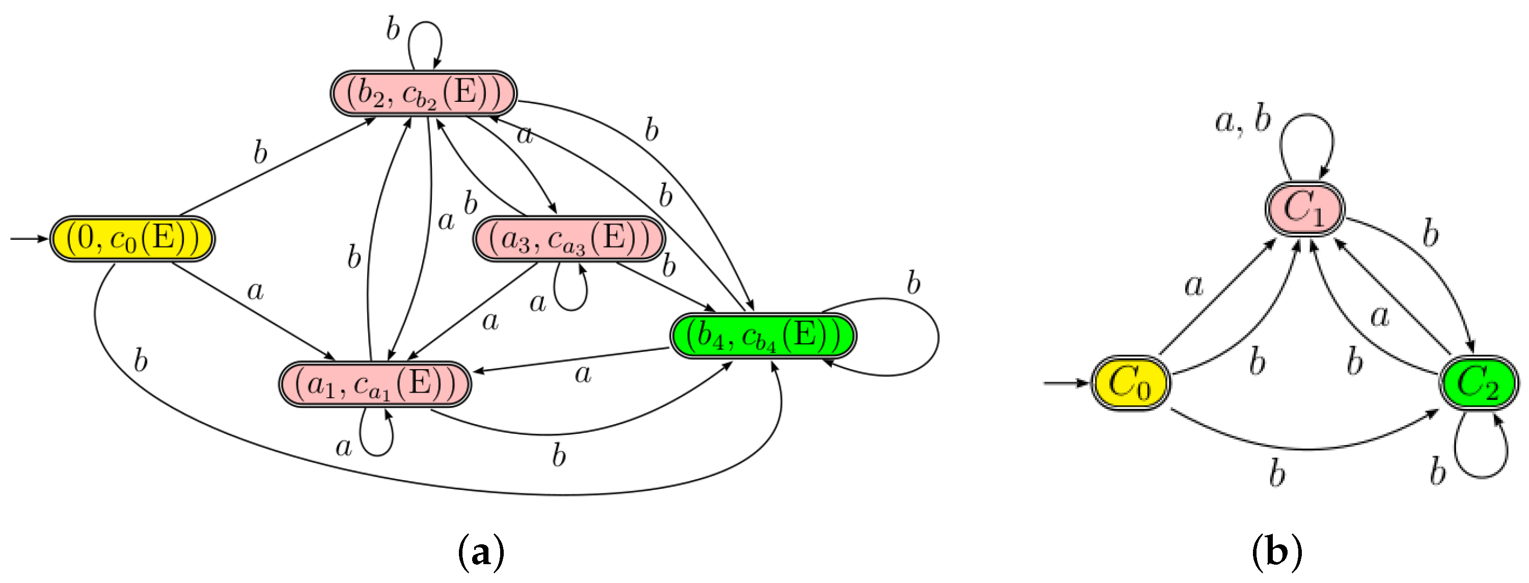
3.1. C-Continuation Automaton

This automaton has been introduced by Champarnaud and Ziadi [6] to efficiently compute the equation automaton. Let us recall the notion of c-derivative, c-continuation and c-continuation automaton.

Definition 1.

(c-derivative with respect to a letter). The c-derivative of a regular expression E with respect to a letter a is the regular expression $d_a(E)$ defined by:

$$\begin{array}{ccc}\hfill d_a(0)& =& d_a(1)=0,\hfill \\ \hfill d_a(x)& =& \mathbf{if}a=x\mathbf{then}1\mathbf{else}0,\hfill \\ \hfill d_a(F+G)& =& \mathbf{if}{d}_a(F)\ne 0\mathbf{then}{d}_a(F)\mathbf{else}{d}_a(G),\hfill \\ \hfill d_a(F·G)& =& \mathbf{if}{d}_a(F)\ne 0\mathbf{then}{d}_a(F)·G\mathbf{else}\lambda (F)·d_a(G),\hfill \\ \hfill d_a(F^{\ast })& =& d_a(F)·F^{\ast }.\hfill \end{array}$$

The c-derivative with respect to a word $u=u_1\cdots u_n$ is defined recursively by the rules: $d_{\epsilon }(E)=E$ and $d_{u_1\cdots u_n}(E)=d_{u_2\cdots u_n}(d_{u_1}(E)).$

Theorem 2.

(Theorem 4 in [6]). Let E be a linear regular expression and a be a letter from E. Then all non-zero c-derivatives of the form $d_{ua}(E)$, where u is an arbitrary word, are equal.

Theorem 2 allows us to define the c-continuation $c_a(E)$ of a in a linear expression E as the unique value of the non-zero c-derivatives $d_{ua}(E)$.

Proposition 1.

(Proposition 6 in [6]). For every letter a of a linear expression E, the c-continuation $c_a(E)$ is such that:

$$\begin{array}{ccc}\hfill c_a(a)& =& 1,\hfill \\ \hfill c_a(F+G)& =& \mathbf{if}{c}_a(F)\mathtt{exists}\mathbf{then}{c}_a(F)\mathbf{else}{c}_a(G),\hfill \\ \hfill c_a(F·G)& =& \mathbf{if}{c}_a(F)\mathtt{exists}\mathbf{then}{c}_a(F)·G\mathbf{else}{c}_a(G),\hfill \\ \hfill c_a(F^{\ast })& =& c_a(F)·F^{\ast }.\hfill \end{array}$$

Corollary 1.

(Corollary 5 in [6]). For every letter a of a linear expression E, the c-continuation $c_a(E)$ is either 1 or a subexpression of E or a product of subexpressions.

More precisely, for a linear regular expression E, we have $c_a(E)=H_0\cdots H_k$, where $H_i$ is a subexpression of E, for all $0\le i\le k$.

We now consider a regular expression E over A. Let $\overline{E}$ be the linearized form of E over $pos(E)$ and h be the mapping from $pos(E)$ onto $A_E$.

In order to simplify the writing for a regular expression E, we consider by convention that $c_0(E)=d_{\epsilon }(\overline{E})=\overline{E}$ and $c_x(E)$ will denote $c_x(\overline{E})$.

Definition 2.

(c-continuation automaton) The c-continuation automaton of E, ${\mathcal{C}}_E=⟨Q,A_E,i,\delta$, $F⟩$, is defined by:

• $Q=\{(x,c_x(E))|x\in pos(E)\cup \{0\}\}$,
• $i=(0,c_0(E))$,
• $F=\{(x,c_x(E))|\lambda (c_x(E))=1\}$,
• $\delta ((x,c_x(E)),a)=\{(y,c_y(E)|h(y)=a and d_y(c_x(E))\equiv c_y(E)\},\forall x\in pos(E)\cup \{0\} and \forall a\in A_E$.

We note that the number of states of ${\mathcal{C}}_E$ is exactly $||E||+1$.

Corollary 2.

(Corollary 7 in [6]). Let E be a regular expression. One has: $L({\mathcal{C}}_E)=L(E)$.

Example 3.

Let us consider the regular expression $E={(a^{\ast }+b{a}^{\ast }+b^{\ast })}^{\ast }$ from Example 1. The linearized form of E is $\overline{E}={(a_1^{\ast }+b_2{a}_3^{\ast }+b_4^{\ast })}^{\ast }$ and the c-continuations of E are as follows:

$\begin{array}{ccc}{c}_0(E)\hfill & =\hfill & {(a_1^{\ast }+b_2{a}_3^{\ast }+b_4^{\ast })}^{\ast }\hfill \\ c_{a_1}(E)\hfill & =\hfill & a_1^{\ast }{(a_1^{\ast }+b_2{a}_3^{\ast }+b_4^{\ast })}^{\ast }\hfill \\ c_{b_2}(E)\hfill & =\hfill & a_3^{\ast }{(a_1^{\ast }+b_2{a}_3^{\ast }+b_4^{\ast })}^{\ast }\hfill \\ c_{b_4}(E)\hfill & =\hfill & b_4^{\ast }{(a_1^{\ast }+b_2{a}_3^{\ast }+b_4^{\ast })}^{\ast }\hfill \end{array}$

$\begin{array}{ccc}{c}_{a_3}(E)\hfill & =\hfill & c_{a_3}(a_1^{\ast }+b_2{a}_3^{\ast }+b_4^{\ast })·{(a_1^{\ast }+b_2{a}_3^{\ast }+b_4^{\ast })}^{\ast }\hfill \\ & =\hfill & c_{a_3}(b_2{a}_3^{\ast })·{(a_1^{\ast }+b_2{a}_3^{\ast }+b_4^{\ast })}^{\ast }\hfill \\ & =\hfill & c_{a_3}(a_3^{\ast })·{(a_1^{\ast }+b_2{a}_3^{\ast }+b_4^{\ast })}^{\ast }\hfill \\ & =\hfill & a_3^{\ast }{(a_1^{\ast }+b_2{a}_3^{\ast }+b_4^{\ast })}^{\ast }\hfill \end{array}$

The outgoing transitions from the state $(0,c_0(E))$ are computed using the c-derivatives of $c_0(E)$ as follows:

$\begin{array}{c}{d}_{a_1}(c_0(E))=c_{a_1}(E),d_{b_2}(c_0(E))=c_{b_2}(E),d_{a_3}(c_0(E))=0,d_{b_4}(c_0(E))=c_{b_4}(E)\hfill \\ d_{a_1}(c_{a_1}(E))=c_{a_1}(E),d_{b_2}(c_{a_1}(E))=c_{b_2}(E),d_{a_3}(c_{a_1}(E))=0,d_{b_4}(c_{a_1}(E))=c_{b_4}(E)\hfill \end{array}$

$\begin{array}{c}{d}_{a_1}(c_{b_2}(E))=c_{a_1}(E),d_{b_2}(c_{b_2}(E))=c_{b_2}(E),d_{a_3}(c_{b_2}(E))=c_{a_3}(E),d_{b_4}(c_{b_2}(E))=c_{b_4}(E)\hfill \end{array}$

$\begin{array}{c}{d}_{a_1}(c_{a_3}(E))=c_{a_1}(E),d_{b_2}(c_{a_3}(E))=c_{b_2}(E),d_{a_3}(c_{a_3}(E))=c_{a_3}(E),d_{b_4}(c_{a_3}(E))=c_{b_4}(E)\hfill \end{array}$

$\begin{array}{c}{d}_{a_1}(c_{b_4}(E))=c_{a_1}(E),d_{b_2}(c_{b_4}(E))=c_{b_2}(E),d_{a_3}(c_{b_4}(E))=0,d_{b_4}(c_{b_4}(E))=c_{b_4}(E)\hfill \end{array}$

Then we get the c-continuation automaton ${\mathcal{C}}_E$ in Figure 4.

Figure 4. The c-continuation automaton ${\mathcal{C}}_E$.

3.2. Equation Automaton as a Quotient of C-Continuation Automaton

Champarnaud and Ziadi [6] have proved that the equation automaton is a quotient of the c-continuation automaton. Let us consider the equivalence relation ${\equiv }_e$ defined by

$$\begin{array}{c}\hfill (x,c_x(E)){\equiv }_e(y,c_y(E))\iff h(c_x(E))\equiv h(c_y(E))\end{array}$$

(1)

Sometimes we write $x{\equiv }_{e}y\iff h(c_x(E))\equiv h(c_y(E))$.

Proposition 2.

The relation ${\equiv }_e$ is right-invariant, i.e., for all letters a in A, for all pairs of states $(x,c_x(E)),(y,c_y(E))$ in Q such that $(x,c_x(E)){\equiv }_e(y,c_y(E))$, we have: $\delta ((x,c_x(E)),a){/}_{{\equiv }_e}=\delta ((y,c_y(E)),a){/}_{{\equiv }_e}$.

Moreover, if two states are equivalent w.r.t. ${\equiv }_e$, then they are either both final or both non-final, since $(x,c_x(E))\in F\iff \lambda (c_x(E))=1\iff \lambda (h(c_x(E)))=1$.

The equivalence class of the state $(x,c_x(E))$ is represented by $C_x=h(c_x(E))$. Since the relation ${\equiv }_e$ is right-invariant, we can define the quotient automaton ${\mathcal{C}}_E{/}_{{\equiv }_e}=⟨Q_{{\equiv }_e},A_E,q_0,\delta ,F⟩$ as follows:

• $Q_{{\equiv }_e}=\{C_x|x\in pos(E)\cup \{0\}\}$,
• $q_0=C_0$,
• $F=\{C_x|\lambda (c_x(E))=1\}$,
• $\delta (C_x,a)=\{C_y|h(y)=a\mathrm{and}{d}_y(c_x(E))\equiv c_y(E)\},\forall C_x\in Q_{{\equiv }_e}\mathrm{and} \forall a\in A_E$.

Theorem 3.

(Theorem 10 in [6]). Let E be a regular expression. The automaton ${\mathcal{C}}_E{/}_{{\equiv }_e}$ deduced from the c-continuation automaton is isomorphic to the equation automaton ${\mathcal{E}}_E$.

We note that the number of states of ${\mathcal{E}}_E$ is majorized by $||E||+1$.

Example 4.

Let us consider the regular expression $E={(a^{\ast }+b{a}^{\ast }+b^{\ast })}^{\ast }$ from Example 1. There are three ${\equiv }_e$-equivalence classes when applying the function h that remove indices from letters for different c-continuations of E:

$\begin{array}{c}h(c_0(E))={(a^{\ast }+b{a}^{\ast }+b^{\ast })}^{\ast }\\ h(c_{a_1}(E))=h(c_{b_2}(E))=h(c_{a_3}(E))=a^{\ast }{(a^{\ast }+b{a}^{\ast }+b^{\ast })}^{\ast }\\ h(c_{b_4}(E))=b^{\ast }{(a^{\ast }+b{a}^{\ast }+b^{\ast })}^{\ast }\end{array}$

The c-continuation automaton ${\mathcal{C}}_E$ and the quotient automaton ${\mathcal{C}}_E{/}_{{\equiv }_e}$ which is isomorphic to the equation automaton ${\mathcal{E}}_E$ are schematized in Figure 5:

Figure 5. (a) The c-continuation automaton ${\mathcal{C}}_E$ versus (b) The quotient automaton ${\mathcal{C}}_E{/}_{{\equiv }_e}$.

4. Allauzen and Mohri’s Algorithm

In [8], Allauzen and Mohri compute the equation automaton from the Thompson automaton of a regular expression E in $O(mlogm+m^2)$ time. Their algorithm is based on some combinations of $\epsilon$-transitions removal and Hopcroft’s algorithm for DFA minimization to the classical Thompson automata [13]. In the next, we briefly describe their method.

Let $\widehat{A}=A_E\cup \{{\epsilon }_{+}^1,{\epsilon }_{+}^2,{\epsilon }_{\ast }^1,{\epsilon }_{\ast }^2\}$. We denote by $\widehat{{\mathcal{T}}_E}$ the automaton over $\widehat{A}$ obtained by recursively marking some of the $\epsilon$-transitions of the Thompson automaton ${\mathcal{T}}_E$ as follows:

Allauzen and Mohri have shown that the equation automaton can be obtained using some $\epsilon$-transitions marking of the Thompson automaton and then apply two classical automata operations, namely epsilon removal, denoted by the function $rmeps$ (resp. the function $\widehat{rmeps}$ for marked epsilon removal) and the Hopcroft’s algorithm for DFA minimization [13], denoted by $mi{n}_{\mathbb{B}}$.

Proposition 3.

(Proposition 3 in [8]). We have ${\mathcal{E}}_E=\widehat{rmeps}(mi{n}_{\mathbb{B}}(rmeps(\widehat{{\mathcal{T}}_E})))$.

Note that after removing $\epsilon$-transitions from the automaton $\widehat{{\mathcal{T}}_E}$, we obtain a deterministic finite automaton $rmeps(\widehat{{\mathcal{T}}_E})$. After that, the Hopcroft’s algorithm for DFA minimization is applied to derive the automaton $mi{n}_{\mathbb{B}}(rmeps(\widehat{{\mathcal{T}}_E}))$ such that the set of its states is in bijection with the set of partial derivatives of E. Finally, to compute transitions of the equation automaton from $mi{n}_{\mathbb{B}}(rmeps(\widehat{{\mathcal{T}}_E}))$, marked $\epsilon$-transitions are removed using $\widehat{rmeps}$ operation.

Theorem 4.

(Theorem 3 in [8]). Let E be a regular expression over A. The equation automaton of E can be computed in $O(mlogm+m^2)$ time.

5. Efficient Conversion Algorithm

In this section, we will show that the equation automaton ${\mathcal{E}}_E$ of a regular expression E can be deduced from the associated Thompson automaton in $O(|E|·|Q_{{\equiv }_e}|)$ time, where $|Q_{{\equiv }_e}|$ denotes the number of states of ${\mathcal{E}}_E$. Algorithm 1 summarizes the different steps of our approach.

Algorithm 1 Computation of the equation automaton.

input: The Thompson automaton ${\mathcal{T}}_E=⟨Q,A_E,I,\delta ,F⟩$ associated with a regular expression E. output:  The equation automaton ${\mathcal{E}}_E$ associated with E. /*           Computation of states                   */

Compute $Id({\mathcal{T}}_E$):

Compute $C_{{\equiv }_e}(Id({\mathcal{T}}_E))$:

• Compute pseudo-continuations for all position states of $Id({\mathcal{T}}_E)$. • Merge equivalent states having the same pseudo-continuation. /*   Computation of transitions and final states              /*

Compute $rmeps(C_{{\equiv }_e}(Id({\mathcal{T}}_E)))$:

• Perform epsilon removal operation using $rmeps()$ function over $C_{{\equiv }_e}(Id({\mathcal{T}}_E))$.

For convenience, we assume that the k states of a given finite automaton are identified by the integers $1,\cdots ,k$.

From Corollary 1, the c-continuation $c_x(E)=H_0\cdots H_l$ associated with a position x is a concatenation of distinct subexpressions $H_i$ of E, possibly reduced to a single subexpression or to 1. In the Thompson automaton ${\mathcal{T}}_E$, we can associate a position x to a particular state q, called position state and define the associated pseudo-continuation $C(q)=N(H_0)\cdots N(H_l)$, where $N(H_i)$ denotes the integer that identify the initial state of the Thompson automaton ${\mathcal{T}}_{H_i}$. So, the first step, compute $Id({\mathcal{T}}_E)$, of our algorithm consists on computing the function $N(.)$ such that for two subexpressions $H_i$ and $H_j$ of E, we have: $H_i\equiv H_j\iff N(I_{{\mathcal{T}}_{H_i}})=N(I_{{\mathcal{T}}_{H_j}})$. This step can be done using a special marking of the $\epsilon$-transitions of ${\mathcal{T}}_E$ that makes it acyclic and deterministic and such that the right languages of its states represent the structure of the corresponding subexpressions. In the next step, Compute $C_{{\equiv }_e}(Id({\mathcal{T}}_E))$, we re-mark the $\epsilon$-transitions such that the resulted automaton is acyclic and deterministic and the right language of a position state in $Id({\mathcal{T}}_E)$ represents a pseudo-continuation. After that, one can merge equivalent position states having the same right language. The final step is the computation of final states and transitions of the equation automaton using an epsilon removal operation, denoted by $rmeps(.)$, from the resulted automaton in the previous step.

In the next, we will show that the equation automaton ${\mathcal{E}}_E$ can be computed efficiently from the Thompson automaton ${\mathcal{T}}_E$ using the following operations $rmeps(C_{{\equiv }_e}(Id({\mathcal{T}}_E)))$.

5.1. Computation of States

In the following, We will show that the computation of the relation ${\equiv }_e$ over the states of the Thompson automaton can be performed in linear time w.r.t. the size of the expression using the minimization of an acyclic deterministic finite automaton. This minimization can be performed efficiently in $O(|E|)$ time using Bubenzer’s algorithm [17,18].

Before computing the equivalence classes $C_{{\equiv }_e}$ over states of the Thompson automaton, we will perform a preprocessing step to identify all identical sub-expressions of E. In the next, we will show that this identification can be done in $O(|E|)$ time.

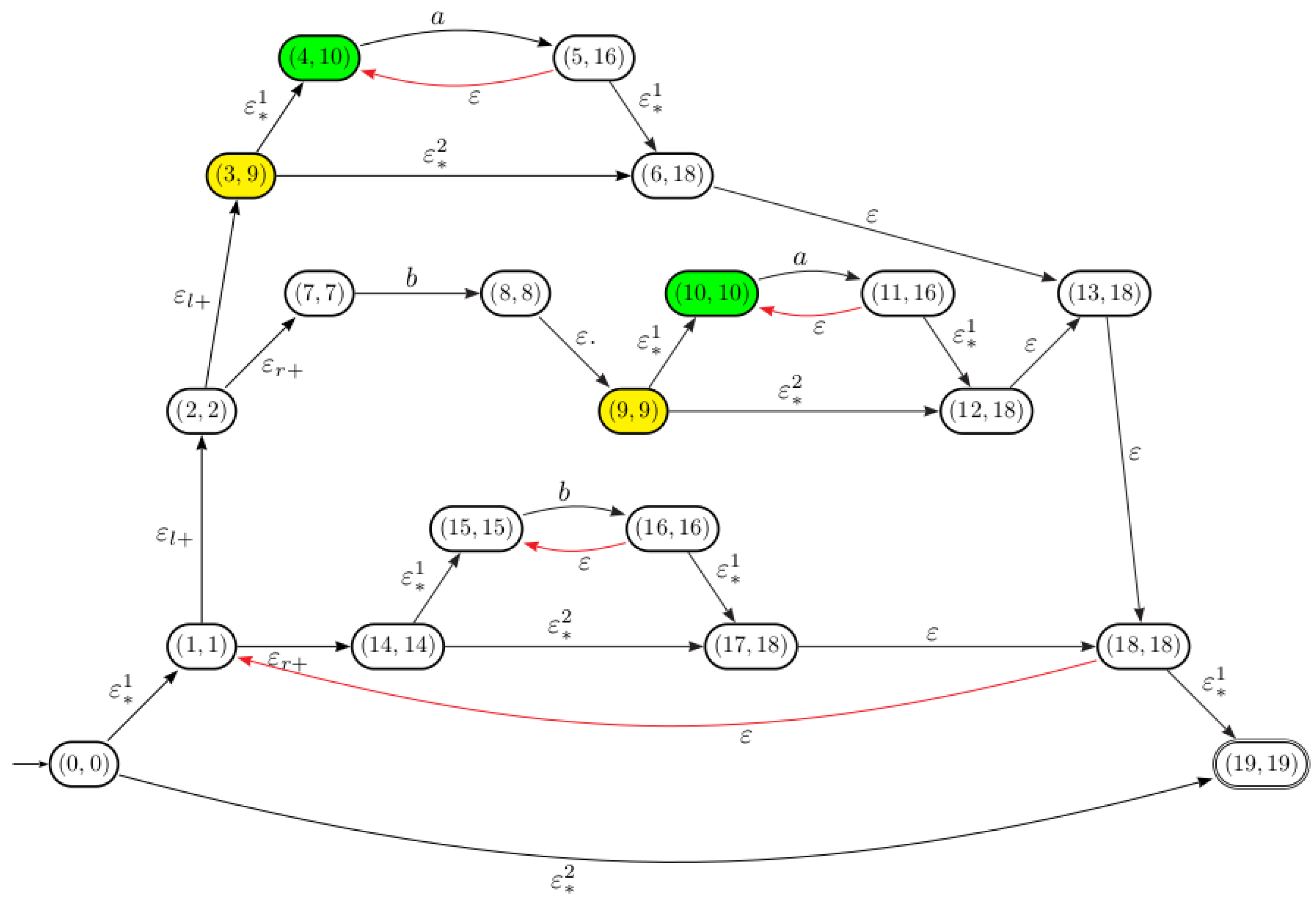
5.1.1. Sub-Expressions Identification

Let Exp the set of all subexpressions of E. In this preprocessing step, we will mark each state in the Thompson automaton by a unique letter in the set $\{1,2,\cdots ,|Exp|\}$.

Let us define a bijection N between the set Exp and a finite set of letters $\{1,2,\cdots ,|Exp|\}$. Consequently, if $E_1$ and $E_2$ are two sub-expressions of E, then we have:

$$E_1\equiv E_2\iff N(E_1)=N(E_2)$$

(2)

Based on the parsing method, introduced in Section 6 in [19], that derive an equivalent regular expression from Thompson automaton, each subexpression $H_i$ of E is associated with an integer identifying the initial state $I_{{\mathcal{T}}_{H_i}}$ in the Thompson automaton ${\mathcal{T}}_E$.

Let q be a state in ${\mathcal{T}}_E$, we denote by $E_q$ the subexpression associated with q, if it exists. For abbreviation, $N(q)$ represents $N(E_q)$.

In the following, we will show that the computation of the function N over the states of ${\mathcal{T}}_E$ turns into a minimization of the acyclic deterministic sub-automaton of the Thompson automaton, $Id({\mathcal{T}}_E)=⟨Q^{\prime },A_E,I,{\delta }^{\prime },F⟩$, defined by:

• $A=\{{\epsilon }_{l+},{\epsilon }_{·},{\epsilon }_{r+},{\epsilon }_{\ast }^1,{\epsilon }_{\ast }^2\}\cup A_E$ where l (resp. r), denote left (resp. right),
• $Q^{\prime }=\{(q,N(q))|q\in Q\}$, i.e., a state in ${\mathcal{T}}_E$ is augmented by the letter $N(q)$.
• The transition function ${\delta }^{\prime }$ is defined over the Thompson automaton as follows:

Notice that this automaton is an acyclic deterministic sub-automaton of the Thompson automaton where $\epsilon$-transitions are indexed and the cyclic transitions in the case when $E=F^{\ast }$ are temporarily disabled.

To compute identical subexpressions, we define the equivalence relation ∼ over the states of $Id({\mathcal{T}}_E)$ as follows:

$$\begin{array}{c}\hfill q\sim q^{\prime }\iff N(q)=N(q^{\prime })\end{array}$$

(3)

Thus we have:

$$\begin{array}{c}\hfill {[q]}_{\sim }={[q^{\prime }]}_{\sim }\iff N(E_q)=N(E_{q^{\prime }})\end{array}$$

(4)

Lemma 1.

Let q and $q^{\prime }$ be two states in $Id({\mathcal{T}}_E)$. We have:

$${\overrightarrow{L}}_q(Id({\mathcal{T}}_E))={\overrightarrow{L}}_{q^{\prime }}(Id({\mathcal{T}}_E))\iff E_q\equiv E_{q^{\prime }}$$

Proof. 

Obvious, by construction. □

Proposition 4.

The function $N(.)$ can be computed over $Id({\mathcal{T}}_E)$ in $O(|E|)$ time.

Proof. 

Let q and $q^{\prime }$ two states in $Id({\mathcal{T}}_E)$. One has:

$$\begin{array}{ccc}q\sim q^{\prime }\hfill & \stackrel{(3)}{⟺}& N(q)=N(q^{\prime })\hfill \\ & \stackrel{(2)}{⟺}& E_q\equiv E_{q^{\prime }}\hfill \\ & \stackrel{Lemma1}{⟺}& {\overrightarrow{L}}_q(Id({\mathcal{T}}_E))={\overrightarrow{L}}_{q^{\prime }}(Id({\mathcal{T}}_E))\hfill \end{array}$$

Thus, the equivalence relation ∼ coincides with Myhill-Nerode equivalence relation [20,21] over the states of $Id({\mathcal{T}}_E)$. Since the automaton $Id({\mathcal{T}}_E)$ is deterministic and acyclic, its minimization using Bubenzer’s algorithm [17] requires $O(|E|)$ time and space complexity. □

Example 5.

The automaton $Id({\mathcal{T}}_E)$ obtained after performing the subexpression identification step for the regular expression $E={(a^{\ast }+b{a}^{\ast }+b^{\ast })}^{\ast }$ through ${\mathcal{T}}_E$.

As shown in Figure 6, for the states 3 and 9 we have:

$$\begin{array}{cc}{\overrightarrow{L}}_3(Id({\mathcal{T}}_E))\hfill & =\{{\epsilon }_{\ast }^{1}a{\epsilon }_{\ast }^1{\epsilon }_{\ast }^1,{\epsilon }_{\ast }^2{\epsilon }_{\ast }^1\}\hfill \\ {\overrightarrow{L}}_9(Id({\mathcal{T}}_E))\hfill & =\{{\epsilon }_{\ast }^{1}a{\epsilon }_{\ast }^1{\epsilon }_{\ast }^1,{\epsilon }_{\ast }^2{\epsilon }_{\ast }^1\}\hfill \end{array}⟺3\sim 9⟺N(3)=N(9)$$

Figure 6. The automaton $Id({\mathcal{T}}_E)$ associated with $E={(a^{\ast }+b{a}^{\ast }+b^{\ast })}^{\ast }$.

As a consequence, we have $E_3\equiv E_9$.

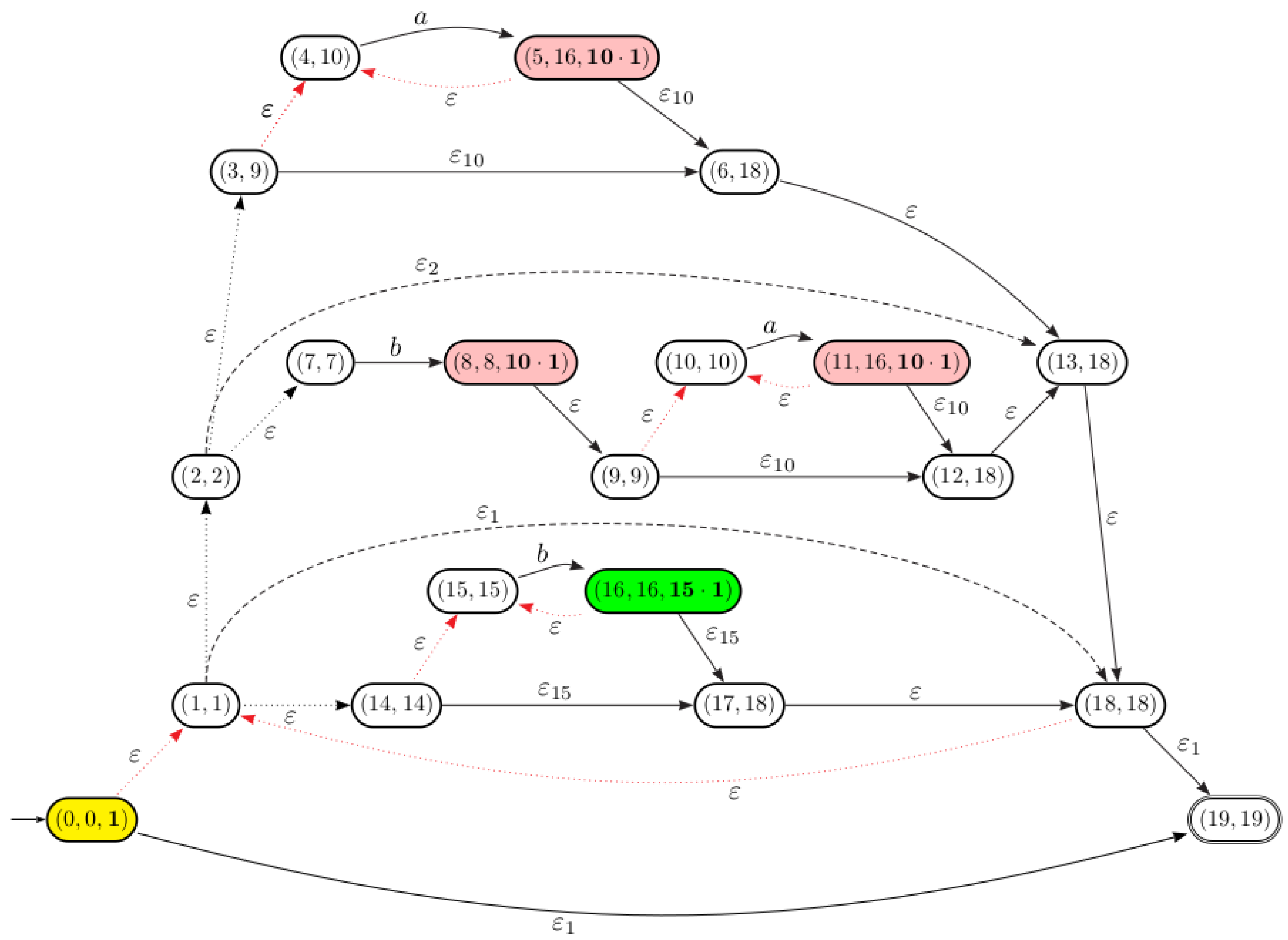
5.1.2. ${\equiv }_e$-Equivalent States Merging

Let us now turn to the computation of the set of states of the equation automaton. From Corollary 1, the c-continuation $c_x(E)$ is a concatenation of distinct subexpressions of E, possibly reduced to a single subexpression or to 1. The following proposition shows that the c-continuation $c_x(E)$ can be computed over the syntactic tree $T(\overline{E})$ associated with the linearized version $\overline{E}$.

Proposition 5.

(Ref. [6]). Let E be a regular expression and x a position in $pos(E)$. Let ${\nu }_x$ be a node in $T(\overline{E})$ such that $\mathit{sym}({\nu }_x)=x$. The c-continuation $c_x(E)$ is as follows:

$$c_x(E)=\underset{\begin{array}{c}{\nu }_x⪯\nu ⪯{\nu }_{\overline{E}}\\ f(\nu )\ne \perp \end{array}}{⨀}{E}_{f(\nu )}$$

where ⊙ is the concatenation operator.

The function $f:\mathit{Nodes}(E)\cup \{\perp \}⟶\mathit{Nodes}(E)\cup \{\perp \}$ is defined as follows:

$$f(\nu )=\left\{\begin{array}{cc}\mathit{father}(\nu )\hfill & if\mathit{sym}(\mathit{father}(\nu ))=\ast and \nu \ne {\nu }_{\overline{E}}\hfill \\ right(\mathit{father}(\nu ))\hfill & if\mathit{sym}(\mathit{father}(\nu ))=·\hfill \\ \perp \hfill & otherwise.\hfill \end{array}\right.$$

with ⊥ is an artificial node such that $f(\perp )=\perp$.

Using Proposition 5, the computation of the set of states requires $O(|E{|}^3)$ time and space complexity. This is due to the fact that the size of a c-continuation is in $O(|E{|}^2)$. In order to reduce this complexity, we introduce a modified definition of pseudo-continuation introduced in [6] over an acyclic deterministic sub-automaton of the Thompson automaton, denoted by $C_{{\equiv }_e}(Id({\mathcal{T}}_E))$. When merging ${\equiv }_e$-equivalent states over $Id({\mathcal{T}}_E)$, we get the automaton $C_{{\equiv }_e}(Id({\mathcal{T}}_E))$. This step requires a linear time w.r.t the size of E using Bubenzer’s algorithm [17], since the automaton $Id({\mathcal{T}}_E)$ is acyclic and deterministic.

In the following, a state $(q,N(q))$ in the automaton $Id({\mathcal{T}}_E)$ is called a position state, if there exists $a\in A_E$ and $(q^{\prime },N(q^{\prime }))\in Q^{\prime }$ such that ${\delta }^{\prime }((q^{\prime },N(q^{\prime })),a)=(q,N(q))$. The state $(0,N(0))$ is also considered as a position state.

It is obvious to see that each position state is associated with a unique position in $pos(E)\cup \{0\}$ and then it’s can be associated with a c-continuation.

Let $(q,N(q))$ and $(q^{\prime },N(q^{\prime }))$ two position states associated with the positions x and $x^{\prime }$ in $pos(E)$. One can extend the ${\equiv }_e$ relation over position states in $Id({\mathcal{T}}_E)$ as follows:

$$\begin{array}{c}\hfill (q,N(q)){\equiv }_e(q^{\prime },N(q^{\prime }))⟺h(c_x(E))\equiv h(c_{x^{\prime }}(E))\end{array}$$

In the next, we will prove that the computation of the equivalence classes $C_{{\equiv }_e}$ can be performed in a linear time w.r.t. the size of the regular expression over $Id({\mathcal{T}}_E)$ using the notion of pseudo-continuations.

For abbreviation, a state $(q,N(q))$ in $Id({\mathcal{T}}_E)$ will be denoted by q. We denote by $C(q)$ the pseudo-continuation associated with the position state q which is an implicit representation of its c-continuation $c_x(E)$, where x is the position letter of q. We will show that the computation of the equivalence classes $C_{{\equiv }_e}$ turns on the computation of pseudo-continuation$C(q)$ over a particular $\epsilon$-transitions marking of the automaton $Id({\mathcal{T}}_E)$.

Definition 3.

The pseudo-continuation $C(q)$ associated with a position state $(q,N(q))\in Q^{\prime }$ in $Id({\mathcal{T}}_E)$ is recursively defined by:

$$\begin{array}{ccc}\hfill C(q)& =& \left\{\begin{array}{cc}N(q)\hfill & if {\delta }^{\prime }(q,{\epsilon }_{l+})=q^{\prime } and {\delta }^{\prime }(q,{\epsilon }_{r+})=q^{″},\hfill \\ N(q^{\prime })·C(q^{″})\hfill & if {\delta }^{\prime }(q,{\epsilon }_1^{\ast })=q^{″} and {\delta }^{\prime }(q^{\prime },a)=q for some a\in A_E,\hfill \\ N(q^{\prime })·C(q^{″})\hfill & if {\delta }^{\prime }(q,{\epsilon }_1^{\ast })=q^{\prime } and {\delta }^{\prime }(q,{\epsilon }_2^{\ast })=q^{″},\hfill \\ a·C(q^{\prime })\hfill & if {\delta }^{\prime }(q,a)=q^{\prime }, for all a\in A_E,\hfill \\ C(q^{\prime })\hfill & if {\delta }^{\prime }(q,\epsilon )=q^{\prime }.\hfill \end{array}\right.\hfill \end{array}$$

(5)

In order to compute efficiently the set of pseudo-continuations associated with the position states in $Id({\mathcal{T}}_E)$, we define an acyclic deterministic sub-automaton $C_{{\equiv }_e}(Id({\mathcal{T}}_E))=⟨Q_{{\equiv }_e},A_E,I,{\delta }^{″},F⟩$ of the Thompson automaton as follows:

• $A=\{{\epsilon }_0,\cdots ,{\epsilon }_{|Exp|}\}\cup A_E$.
• $Q_{{\equiv }_e}=\{(q,C(q))|(q,N(q))\in Q^{\prime }\}$, i.e., a state in $Id({\mathcal{T}}_E)$ is replaced by $(q,C(q))$.
• The transition function ${\delta }^{″}$ is defined as follows:

Let us define the equivalence relation ≈ over the position states of $C_{{\equiv }_e}(Id({\mathcal{T}}_E))$ as follows:

$$\begin{array}{c}\hfill (q,C(q))\approx (q^{\prime },C(q^{\prime }))\iff C(q)\equiv C(q^{\prime })\end{array}$$

(6)

Thus we have:

$$\begin{array}{c}\hfill {[q]}_{\approx }={[q^{\prime }]}_{\approx }\iff C(q)\equiv C(q^{\prime })\end{array}$$

(7)

Let $\overline{h}$ be the application that maps a letter ${\epsilon }_i$ to the letter i. By construction, the following proposition holds.

Proposition 6.

Let $(q,C(q))$ be a position state in $C_{{\equiv }_e}(Id({\mathcal{T}}_E))$. We have:

$$\overline{h}({\overrightarrow{L}}_q(C_{{\equiv }_e}(Id({\mathcal{T}}_E))))=C(q)$$

Example 6.

Let us consider the Thompson automaton ${\mathcal{T}}_E$ defined in previous examples. Figure 7 schematizes the derived automaton from $Id({\mathcal{T}}_E)$ after pseudo continuations computation for position states.

Figure 7. Pseudo-continuations computation for position states in $Id({\mathcal{T}}_E)$.

Notice that dotted ε-transitions are temporarily disabled and dashed ones are temporarily added.

The position states in the automaton $Id({\mathcal{T}}_E)$ are $\{0,5,8,11,16\}$. According to the definition of a pseudo continuation (see Formula (7)), the pseudo-continuations associated with position states are computed over the automaton $Id({\mathcal{T}}_E)$ as follows:

$$\begin{array}{c}C(5)=C(8)=C(11)=10·1\hfill \\ C(16)=15·1\hfill \end{array}$$

On the other hand, we have:

$$\begin{array}{c}{\overrightarrow{L}}_5(C_{{\equiv }_e}(Id({\mathcal{T}}_E)))={\overrightarrow{L}}_8(C_{{\equiv }_e}(Id({\mathcal{T}}_E)))={\overrightarrow{L}}_{11}(C_{{\equiv }_e}(Id({\mathcal{T}}_E)))={\epsilon }_{10}·{\epsilon }_1\hfill \\ {\overrightarrow{L}}_{16}(C_{{\equiv }_e}(Id({\mathcal{T}}_E)))={\epsilon }_{15}·{\epsilon }_1\hfill \end{array}$$

The following proposition is fundamental to prove that the equivalence relation ${\equiv }_e$ using the notion of c-continuation is the same when using pseudo-continuations $C(q)$.

Proposition 7.

Let q (resp. $q^{\prime }$) be a position state associated with a position $x\in pos(E)$ (resp. $x^{\prime }\in pos(E)$) in $C_{{\equiv }_e}(Id({\mathcal{T}}_E))$. One has:

$$C(q)\equiv C(q^{\prime })\iff h(c_x(E))\equiv h(c_{x^{\prime }}(E))$$

As a consequence, the following proposition holds.

Proposition 8.

Let q and $q^{\prime }$ be two position states in $C_{{\equiv }_e}(Id({\mathcal{T}}_E))$. One has:

$$q{\equiv }_e{q}^{\prime }\iff C(q)\equiv C(q^{\prime })$$

Theorem 5.

Let E be a regular expression and ${\mathcal{T}}_E$ the associated Thompson automaton. The relation ${\equiv }_e$ can be computed over $C_{{\equiv }_e}(Id({\mathcal{T}}_E))$ in $O(|E|)$ time.

Proof. 

From Proposition 8, one can deduce that the computation of the equivalence relation ${\equiv }_e$, turn to apply the Myhill-Nerode relation on the states of the automaton $C_{{\equiv }_e}(Id({\mathcal{T}}_E))$. By definition, this last is acyclic and deterministic. Then, its minimization using Bubenzer’s algorithm [17] requires $O(|E|)$ time and space complexity. □

Example 7

(Continues). The automaton $C_{{\equiv }_e}(Id({\mathcal{T}}_E))$, schematized in the Figure 8, is obtained from $Id({\mathcal{T}}_E)$ after merging ${\equiv }_e$-equivalent position states $5,8$ and 11.

Figure 8. The automaton $C_{{\equiv }_e}(Id({\mathcal{T}}_E))$ associated with $E={(a^{\ast }+b{a}^{\ast }+b^{\ast })}^{\ast }$.

The next step of our approach consists of the transitions and final states computation of the equation automaton ${\mathcal{E}}_E$ using epsilon removal operation, denoted by $rmeps()$, over the automaton $C_{{\equiv }_e}(Id({\mathcal{T}}_E))$.

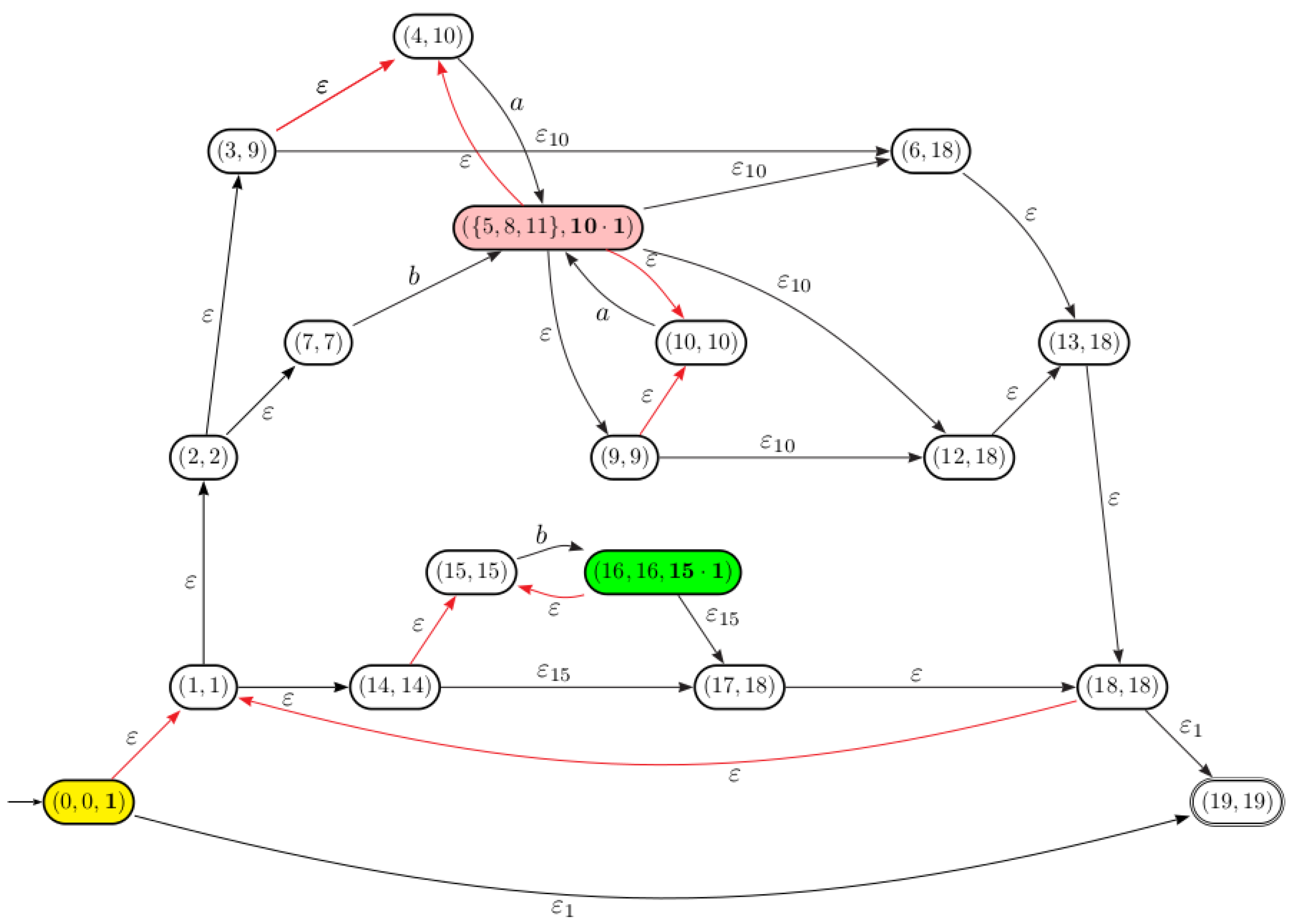
5.2. Computation of Transitions and Final States

After merging ${\equiv }_e$-equivalent states in the previous step, we obtain a reduced automaton $C_{{\equiv }_e}(Id({\mathcal{T}}_E))$ having the same set of states as the equation automaton. To compute the transition function, we first enable the cyclic transitions previously disabled in the case when $E=F^{\ast }$ on $C_{{\equiv }_e}(Id({\mathcal{T}}_E))$.

Let $Q_{{\equiv }_e}$ be the set of states of $C_{{\equiv }_e}(Id({\mathcal{T}}_E))$. Recall that epsilon removal operation is denoted by, $rmeps(p)$ for a state $p\in Q$ and $rmeps(\mathcal{A})$ denotes the resulted automaton after removing marked and non-marked $\epsilon$-transitions from the automaton $\mathcal{A}$.

As a consequence of Lemma 5 from [8], the following Lemma yeilds.

Lemma 2.

(Lemma 5 in [8]). Let q and $q^{\prime }$ be two position states in $Q_{{\equiv }_e}$ associated respectively with the positions x and $x^{\prime }$ in $pos(E)\cup \{0\}$, we have:

$$q\in rmeps(q^{\prime }) iff h(c_x(E))\in {\partial }_a(h(c_{x^{\prime }}(E))), for some a\in A_E.$$

The set of destination states of the outgoing transitions from a state $q\in Q_{{\equiv }_e}$ is then equal to

$$\{p\in Q_{{\equiv }_e}|p\in rmeps(q) \mathrm{and} p \mathrm{is} \mathrm{a} \mathrm{position} \mathrm{state}\}$$

Lemma 3.

Let q be a position state in $Q_{{\equiv }_e}$ associated with a position x in $pos(E)\cup \{0\}$, we have:

$$F\in rmeps(q) iff \lambda (c_x(E))=1.$$

Proposition 9.

We have ${\mathcal{E}}_E=rmeps(C_{{\equiv }_e}(Id({\mathcal{T}}_E)))$

Example 8.

(Continues). Let us consider the automaton $C_{{\equiv }_e}(Id({\mathcal{T}}_E))$ of the Example 7. The final states and the transitions of the equation automaton are computed over $C_{{\equiv }_e}(Id({\mathcal{T}}_E))$ using epsilon removal operation $rmeps$ as follows:

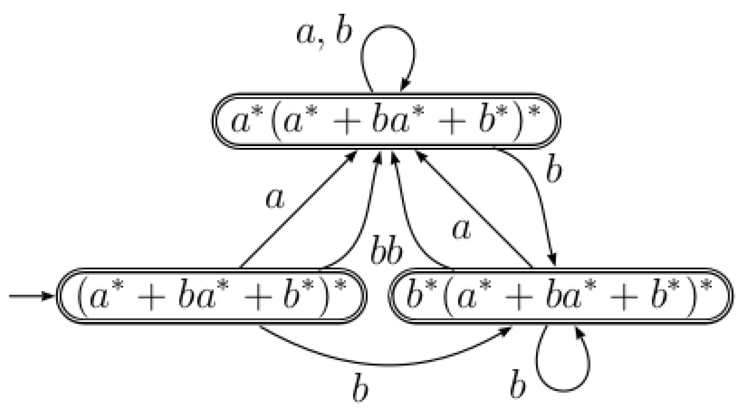
• The set of states of the equation automaton are $\{0,\{5,8,11\},16\}$.
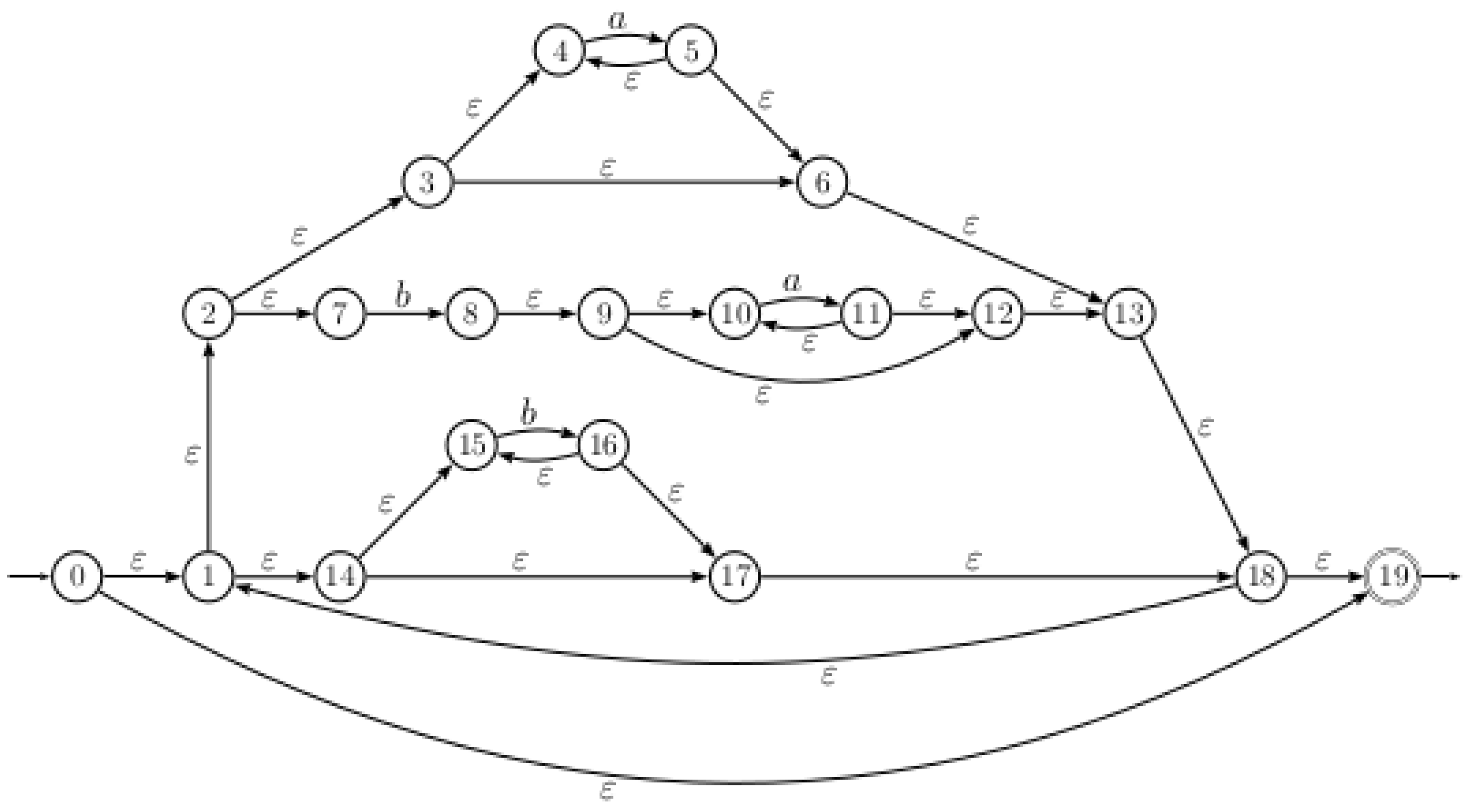
• Since the final state of $C_{{\equiv }_e}(Id({\mathcal{T}}_E))$ is the state 19 and $19\in rmeps(0)$, $19\in rmeps(\{5,8,11\})$, and $19\in rmeps(16)$, then the set of final states are $\{0,\{5,8,11\},16\}$.
• There are two paths in $C_{{\equiv }_e}(Id({\mathcal{T}}_E))$ from the state 0 to the state $\{5,8,11\}$ labeled respectively by $\epsilon ·\epsilon ·\epsilon ·\epsilon ·a$ and $\epsilon ·\epsilon ·\epsilon ·b$, then $\{5,8,11\}\in rmeps(0)$. Consequently, two transitions $(0,a,\{5,8,11\})$ and $(0,b,\{5,8,11\})$ are added to the equation automaton. The same process will be applied for other transitions.

Since there are $O(|E|)$ states in $C_{{\equiv }_e}(Id({\mathcal{T}}_E))$ and the operation $rmeps(C_{{\equiv }_e}(Id({\mathcal{T}}_E)))$ is performed on exactly $|Q_{{\equiv }_e}|$ states, the following theorem holds.

Theorem 6.

Let E be a regular expression. The equation automaton of E can be computed in $O(|E|·|Q_{{\equiv }_e}|)$.

6. Conclusions

In this paper, we presented a fast and sophisticated construction of the equation automaton from a regular expression over its associated Thompson automaton. The time complexity of our algorithm is at least as favorable as that of the best previously known algorithm. It is based on the minimization of acyclic deterministic finite automata and epsilon removal operations. This allowed us a construction of the equation automaton in $O(|E|·|Q_{{\equiv }_e}|)$ time and space complexity where $|Q_{{\equiv }_e}|$ denotes the number of transitions of the produced automaton. The implementation of the proposed algorithm is available under the following repository: https://github.com/FaissalOuardi/Equation-automaton (accessed on 27 May 2021).

References

- Mirkin, B.G. Novyj algoritm postroéniá bazisa v ázyké régularnyh vyražénij. Izvéstiá Akadémii Nauk SSSR. Engineering cybernetics, no. 5 (1966). English translation of the preceding: Brzozowski, J. An algorithm for constructing a base in a language of regular expressions. pp. 110–116. J. Symb. Log. 1971, 36, 694. [Google Scholar]
- Antimirov, V. Partial derivatives of regular expressions and finite automaton constructions. Theor. Comput. Sci. 1996, 155, 291–319. [Google Scholar] [CrossRef]
- Glushkov, V.M. The abstract theory of automata. Russ. Math. Surv. 1961, 16, 1–53. Available online: https://iopscience.iop.org/article/10.1070/RM1961v016n05ABEH004112 (accessed on 27 May 2021). [CrossRef]
- McNaughton, R.F.; Yamada, H. Regular expressions and state graphs for automata. IEEE Trans. Electron. Comput. 1960, 9, 39–57. [Google Scholar] [CrossRef]
- Ziadi, D.; Ponty, J.-L.; Champarnaud, J.-M. A New Quadratic Algorithm to Convert a Regular Expression into an Automaton. In Proceedings of the Workshop on Implementing Automata, London, ON, Canada, 29–31 August 1996; pp. 109–119. [Google Scholar]
- Champarnaud, J.-M.; Ziadi, D. Canonical derivatives, partial derivatives and finite automaton constructions. Theor. Comput. Sci. 2002, 289, 137–163. [Google Scholar] [CrossRef]
- Khorsi, A.; Ouardi, F.; Ziadi, D. Fast equation automaton computation. J. Discret. Algorithms 2008, 6, 433–448. [Google Scholar] [CrossRef][Green Version]
- Allauzen, C.; Mohri, M. A Unified Construction of the Glushkov, Follow, and Antimirov Automata. In Proceedings of the International Conference of Mathematical Foundations of Computer Science, Stará Lesná, Slovakia, 28 August–1 September 2006; pp. 110–121. [Google Scholar]
- Ilie, L.; Yu, S. Follow automata. Inf. Comput. 2003, 186, 140–162. [Google Scholar] [CrossRef]
- Champarnaud, J.-M.; Nicart, F.; Ziadi, D. From the ZPC Structure of a Regular Expression to its Follow Automaton. IJAC 2006, 16, 17–34. [Google Scholar] [CrossRef]
- Kleene, S. Representation of Events in Nerve Nets and Finite Automata; Automata Studies, Ann. Math. Studies 34; Princeton University Press: Princeton, NJ, USA, 1956; pp. 3–41. [Google Scholar]
- Thompson, K. Regular Expression Search Algorithm. Commun. ACM 1968, 11, 410–422. [Google Scholar] [CrossRef]
- Hopcroft, J. An n log n Algorithm for Minimizing States in a Finite Automaton; Technical Report; Stanford University, CS Dept.: Stanford, CA, USA, 1971. [Google Scholar]
- Hopcroft, J.E.; Ullman, J.D. Introduction to Automata Theory, Languages and Computation; Addison-Wesley: Reading, MA, USA, 1979. [Google Scholar]
- Sakarovitch, J.; Thomas, R. Elements of Automata Theory; Cambridge University Press: Cambridge, UK, 2009. [Google Scholar]
- Brüggemann-Klein, A. Regular expressions into finite automata. Theor. Comp. Sci. 1993, 120, 117–126. [Google Scholar] [CrossRef]
- Bubenzer, J. Cycle-aware minimization of acyclic deterministic finite-state automata. J. Discret. Appl. Math. 2014, 163, 238–246. [Google Scholar] [CrossRef]
- Revuz, D. Minimization of acyclic deterministic automata in linear time. Theor. Comput. Sci. 1992, 92, 181–189. [Google Scholar] [CrossRef]
- Giammarresi, D.; Ponty, J.-L.; Wood, D.; Ziadi, D. A characterization of Thompson digraphs. Discret. Appl. Math. 2004, 134, 317–337. [Google Scholar] [CrossRef]
- Myhill, J. Finite automata and the representation of events. In WADD TR-57-624; Wright Patterson AFB: Dayton, OH, USA, 1957; pp. 112–137. [Google Scholar]
- Nerode, A. Linear automata transformation. Proc. AMS 1958, 9, 541–544. [Google Scholar] [CrossRef]
Publisher’s Note: MDPI stays neutral with regard to jurisdictional claims in published maps and institutional affiliations. |
© 2021 by the authors. Licensee MDPI, Basel, Switzerland. This article is an open access article distributed under the terms and conditions of the Creative Commons Attribution (CC BY) license (https://creativecommons.org/licenses/by/4.0/).