Interactive Graph Stream Analytics in Arkouda

Abstract

Data from emerging applications, such as cybersecurity and social networking, can be abstracted as graphs whose edges are updated sequentially in the form of a stream. The challenging problem of interactive graph stream analytics is the quick response of the queries on terabyte and beyond graph stream data from end users. In this paper, a succinct and efficient double index data structure is designed to build the sketch of a graph stream to meet general queries. A single pass stream model, which includes general sketch building, distributed sketch based analysis algorithms and regression based approximation solution generation, is developed, and a typical graph algorithm—triangle counting—is implemented to evaluate the proposed method. Experimental results on power law and normal distribution graph streams show that our method can generate accurate results (mean relative error less than 4%) with a high performance. All our methods and code have been implemented in an open source framework, Arkouda, and are available from our GitHub repository, Bader-Research. This work provides the large and rapidly growing Python community with a powerful way to handle terabyte and beyond graph stream data using their laptops.

1. Introduction

More and more emerging applications, such as social networks, cybersecurity and bioinformatics, have data that often come in the form of real-time graph streams [1]. Over its lifetime, the sheer volume of a stream could be petabytes, or more like network traffic analysis in the IPv6 network, which has $2^{128}$ nodes. These applications motivate the challenging problem of designing succinct data structures and real-time algorithms to return approximate solutions. Different stream models [2,3,4,5,6,7], which allow access to the data in only one pass (or multi-pass in semi-streaming algorithms), are developed to answer different queries using a significantly reduced sublinear space. The accuracy of such models’ approximate solutions is often guaranteed by a pair of user specified parameters, $ϵ>0$ and $0<\delta <1$. This means that the $(1+ϵ)$ approximation ratio can be achieved with a probability of $(1-\delta )$. This literature provides the theoretical foundation to solve the challenging large scale stream data problem.

However, ignoring the hidden constants in the theoretical space and time complexity analysis can cause unacceptable performance problems in real-world applications. When different applications, such as from social, economic and natural domains, have to handle real-time large data streams as routine work, the practical performance for real-world applications becomes an even more important and urgent requirement.

At the same time, graph streams need exploratory data analysis (EDA) [8,9,10]. Instead of checking results, given a hypothesis, with data, EDA is primarily for seeing what the data can tell us beyond the formal modeling or hypotheses testing task. In this way, EDA tries to maximize the value of data. Popular EDA methods and tools, which often run on laptops or common personal computers, cannot hold terabyte or even larger graph datasets, let alone produce highly efficient analysis results. Arkouda [11,12] is an EDA framework under early development that brings together the productivity of Python with world-class high-performance computing. If a graph stream algorithm can be integrated into Arkouda, it means that data scientists can take advantage of both laptop computing and cloud/supercomputing to perform interactive data analysis at scale.

In this work, we propose a single pass stream model and develop a typical algorithm for interactive graph stream analytics that can meet practical performance requirements with high accuracy. Furthermore, the proposed model and algorithm will be integrated into Arkouda to support the Python community to handle graph streams efficiently. The major contributions of this paper are as follows:

• A succinct Double-Index (DI) data structure is designed to build the sketch of a large graph stream. The DI data structure can support an edge based sparse graph partition to achieve load balance and to achieve $\mathcal{O}\left(1\right)$ time complexity in searching the incidence vertices of a given edge or the adjacency list of a given vertex.
• A single pass regression analysis stream model is developed to support general graph streams analysis. Our model can map a large graph stream into a much smaller user specified working space to build a general graph stream sketch. Our method can improve the query quality by dividing the sketch into multiple partitions. A general regression method is proposed to generate the approximate solution based on the partial query results from different partitions.
• A typical graph algorithm—triangle counting [13]—is developed to evaluate the efficiency of the proposed stream regression model. Experimental results using two typical distributions—power law and normal distributions—show that our method can achieve a high accuracy with a very low (4%) mean relative error.
• All the proposed methods have been integrated into an open-source framework, Arkouda, to evaluate their practical end-to-end performance. This work can help the large and popular data analytics community that exists within Python to conduct interactive graph stream analytics easily and efficiently on terabytes, and beyond, of graph stream data.

2. Related Work

There are two different methods for handling graph streams. One is the exact method and the other is the approximate method. The exact method needs very large memory to completely hold the graph stream. This is often not feasible for hardware resource limited systems. The approximate method will use very limited memory (sublinear space) to handle the graph streams but can only provide approximate solutions. In this section, we will introduce the related approximate methods, exact methods and different triangle counting algorithms.

2.1. Graph Stream Sketch

A much smaller sketch allows for many queries over the large graph stream to obtain approximate results efficiently. Therefore, how to build a graph stream’s sketch is of fundamental importance for graph stream analytics. There are several methods that build the sketch by treating each stream element independently without keeping the relationships among those elements. For example, CountMin [4] allows fundamental queries in data stream summarization such as point, range, and inner product queries. It can also be used to find quantiles and frequent items in a data stream. Bottom K sketch [5] places both priority sampling and weighted sampling, without replacement, within a unified framework. It can generate tighter bounds when the total weight is available. gSketch [6] introduces the sketch partitioning technique to estimate and optimize the responses to basic queries on graph streams. By exploiting both data and query workload samples, gSketch can achieve better query estimation accuracy than that achieved with only the data sample. In fact, we borrow the sketch partitioning idea in our implementation of the Double-Index (DI) sketch. However, these existing sketches focus on ad-hoc problems (they can only solve the proposed specific problems instead of general problems), so they cannot support general data analytics over graph streams.

TCM sketch [7] uses a graphical model to build the sketch of a graph stream. This means that TCM is a general sketch that allows complicated queries. However, TCM’s focus is setting up a general sketch theoretically, instead of optimizing the practical performance for real-world datasets. Our Double-Index (DI) sketch is especially designed for real-world sparse graph streams and it can achieve a high practical performance.

2.2. Complete Graph Stream Processing Method

Several dynamic graph management and analytics solutions are as follows. Aspen [14] takes advantage of purely functional trees data structure, C-trees, to implement quick graph updates and queries. LLAMA’s streaming graph data structure [15] is motivated by the CSR format. However, like Aspen, LLAMA is designed for batch processing in the single-writer multi-reader setting and does not provide graph mutation support. GraphOne [16] can run queries on the most recent version of the graph while processing updates concurrently by using a combination of an adjacency list and an edge list.

Systems such as LLAMA, Aspen and GraphOne focus on designing efficient dynamic graph data structures, and their processing units do not support incremental computation. KickStarter [17] maintains the dependency information in the form of dependency trees, and performs an incremental trimming process that adjusts the values based on monotonic relationships. GraphBolt [18] incrementally processes streaming graphs and minimizes redundant computations upon graph mutations while still guaranteeing synchronous processing semantics. DZiG [19] is a high-performance streaming graph processing system that retains efficiency in the presence of sparse computations while still guaranteeing BSP semantics. However, all such methods have the challenging requirement that the memory must be large enough to hold all the streams. For very large streams, this is often not feasible.

2.3. Triangle Counting Algorithm

Triangle counting is a key building block for important graph algorithms such as transitivity and K-truss. There are two kinds of triangle counting algorithms, exact triangle counting for static graphs and approximate triangle counting for graphs built from dynamic streams [1]. Since the proposed DI sketch is a graphical model, all the static triangle counting algorithms can also be used on the small DI sketch.

Graph Challenge https://graphchallenge.mit.edu/challenges (accessed on 20 July 2021) is an important competition for large graph algorithms (including triangle counting). Starting from 2017, many excellent static triangle counting algorithms have been developed. They target three hardware platforms: shared memory, distributed memory and GPU.

The shared memory methods take advantage of some fast parallel packages, such as Kokkos Kernels [20] or Cilk [21], to improve their performance. However, the GPU methods [22,23,24] use massively parallel fine-grain hardware threads of a GPU to improve the performance. Distributed memory triangle counting focuses on very large graphs that cannot fit in a single node’s memory. Some heuristics [25], optimized communication libraries [26] and graph structures [27] are used to improve the performance. We leverage the ideas in such methods to develop our Chapel-based multi-locale triangle counting algorithm.

The basic idea of graph stream analysis is to estimate the exact query result of a graph stream based on the sampling results. Colorful triangle counting [28] is an example. However, it needs to know the number of triangles and the maximum number of triangles of an edge to set the possibility value. This is not feasible in practical applications. Reduction-based [29] triangle counting is a typical method, which can design a theoretical algorithm based on user specified values $(ϵ,\delta )$. Such a method often cannot directly be used satisfactorily in practical applications because hidden constant values often impact the performance. Neighborhood sampling [30] is another method for triangle counting with significant space and time complexity improvements. Specifically, Braverman et al. [31] discuss the difficulty of the triangle counting algorithm in a streaming model. Other sampling methods, such as [32], have space usage that depends on the ratio of the number of triangles and the number of triples, or the algorithm will require the edge stream to meet a specific order. Jha et al. [33] apply the birthday paradox theory to sampling data to estimate the number of triangles in a graph stream.

3. Arkouda Framework

Arkouda is an open-source framework that aims to support flexible, productive, and high performance large scale data analytics. The basic building components of Arkouda include three parts: the front-end (Python [34]), the back-end (Chapel [35]) and a middle, communicative part (ZeroMQ [36]). Python is the interface for end users to utilize the different functions from Arkouda. All large data analysis and high performance computing (HPC) tasks are executed at the back-end (server) without users needing to know the algorithmic implementation details. ZeroMQ is used for the data and instruction exchanges between Python users and the Chapel back-end services.

In order to enable exploratory data analysis on large scale datasets in Python, Arkouda divides its data into two physical sections. The first section is the metadata, which only include attribute information and occupy very little memory space. The second section is the raw data, which include the actual big datasets to be handled by the back-end. However, from the view of the Python programmers, all data are directly available just as on their local laptop device. This is why Arkouda can break the limit of local memory capacity, while at the same time bringing traditional laptop users powerful computing capabilities that could previously only be provided by supercomputers.

When users are exploring their data, if only the metadata section is needed, then the operations can be completed locally and quickly. These actions are carried out just as in previous Python data processing workflows. If the operations have to be executed on raw data, the Python program will automatically generate an internal message and send the message to Arkouda’s message processing pipeline for external and remote help. Arkouda’s message processing center (ZeroMQ) is responsible for exchanging messages between its front-end and back-end. When the Chapel back-end receives the operation command from the front-end, it will execute the analysis task quickly on the powerful HPC resources and large memory to handle the corresponding raw data and return the required information back to the front-end. Through this, Arkouda can support Python users to locally handle large scale datasets residing on powerful back-end servers without knowing all the detailed operations at the back-end.

Figure 1 is a schematic diagram visualizing how Arkouda can bridge the popularity of Python and the power of HPC together to enable EDA at scale. In this figure, from the conceptual level view, Arkouda has three loosely coupled components. The different components can be designed and implemented independently as long as they follow the same information exchanging interface. Although Arkouda is implemented using Chapel, ZeroMQ and Python, the basic concepts can be implemented with different languages and packages. From the view of data, the data are classified into two categories, metadata and raw data. Correspondingly, we simply refer to the operations that can be done locally and quickly as light operations. The operations that need help from the remote server or data center are referred to as heavy operations. Arkouda can automatically organize the data and the corresponding operations to provide a better performance and user experience.

Figure 1. Overview of Arkouda’s components and working mechanism.

In this paper, we discuss the integration of our graph stream sketch, model and algorithm into Arkouda to enable popular and high level Python users to conduct interactive graph stream analytics.

4. Succinct Data Structure

4.1. Edge Index and Vertex Index

We propose a Double-Index (DI) data structure to support quick search from a given edge to its incident vertices or from a given vertex to its adjacency list. The two index arrays are called the edge index array and the vertex index array. Furthermore, our DI data structure requires a significantly smaller memory footprint for sparse graphs.

The edge index array consists of two arrays with the same shape. One is the source vertex array and the other is the destination vertex array. If there are a total of M edges and N vertices, we will use the integers from 0 to $M-1$ to identify different edges and the integers from 0 to $N-1$ to identify different vertices. For example, given edge $e=⟨i,j⟩$, we will let $SRC\left[e\right]=i$ and $DST\left[e\right]=j$, where $SRC$ is the source vertex array and $DST$ is the destination vertex array; e is the edge ID number. Both $SRC$ and $DST$ have the same size M. When all edges are stored in $SRC$ and $DST$, we will sort them based on their combined vertex ID value $\left(SRC\right[e],DST[e\left]\right)$, and remap the edge ID from 0 to $M-1$. Based on the sorted edge index array, we can build the vertex index array, which also consists of two of the same shape arrays. For example, in Figure 2, we let edge $e_{1000}$ have ID 1000. If $e_{1000}=⟨50,3⟩$, $e_{1001}=⟨50,70⟩$ and $e_{1002}=⟨50,110⟩$ are all the edges starting from vertex 50 (a directed graph). Then we will let one vertex index array $STR\left[50\right]=1000$ and another vertex index array $NEI\left[50\right]=3$. This means that, for given vertex ID 50, the edges starting with vertex 50 are stored in the edge index array starting at position 1000 and there is a total of 3 such edges. If there are no edges from vertex i, we will let $STR\left[i\right]=-1$ and $NEI\left[i\right]=0$. In this way, we can directly search the neighbors or adjacency list of any given vertex.

Figure 2. Double Index data structure for graph stream sketch.

Our DI data structure can also support graph weights. If each vertex has a different weight, we use an array, $V\_WEI$, to express the weight values. If each edge has a weight, we use an array, $E\_WEI$, to store the different weights.

4.2. Time and Space Complexity Analysis

For a given array A, we use $A[i..j]$ to express the elements in A from $A\left[i\right]$ to $A\left[j\right]$. $A[i..j]$ is also called an array section of A. So, for a given vertex with index i, it will have $NEI\left[i\right]$ neighbors and their vertex IDs are from $DST\left[STR\right[i\left]\right]$ to $DST\left[STR\right[i]+NEI[i]-1]$. This can be expressed as an array section $DST\left[STR\right[i]..STR[i]+NEI[i]-1]$ (here we assume the out degree of i is not 0). For given vertex i, the adjacency list of vertex i can be easily expressed as $⟨i,x⟩$, where x in $DST\left[STR\right[i]..STR[i]+NEI[i]-1]$. Based on the $NEI$ and $STR$ vertex index arrays, we can find the neighbor vertices or the adjacency list in $\mathcal{O}\left(1\right)$ time complexity. For given edge $e=⟨i,j⟩$, it will be easy for us to find its incident vertices i in array $SRC\left[e\right]$ and j in array $DST\left[e\right]$ and also in $\mathcal{O}\left(1\right)$ time complexity. Regarding the storage space, if the graph has M edges and N vertices, we will need $2M$ memory to store all the edges. Compared with the dense matrix data structure, which needs $N^2$ memory to store all the edges, this is much smaller. To improve the adjacency list search performance, we use $2N$ memory to store the $NEI$ and $STR$ arrays.

Figure 2 shows M sorted edges represented by the $SRC$ and $DST$ arrays. Any one of the N vertices $n_k$ can find its neighbors using $NEI$ and $STR$ arrays with $\mathcal{O}\left(1\right)$ time complexity. For example, given edge $⟨i,j⟩$, if vertex j’s starting index in $SRC$ is 1000, it has three adjacency edges, then such edges can be found starting from index position 1000 in arrays $SRC$ and $DST$ using $NEI$ and $STR$ arrays directly. This figure shows how the $NEI$ and $STR$ arrays can help us locate neighbors and adjacency lists quickly.

For an undirected graph, an edge $⟨i,j⟩$ means that we can also arrive at i from j. We may use the data structures $SRC,DST,STR,NEI$ to search the neighbors of j in SRC. However, this search cannot be performed in $\mathcal{O}\left(1\right)$ time complexity. To improve the search performance, we introduce another four arrays, called reversed arrays, $SRCr,DSTr,STRr,NEIr$. For any edge $⟨i,j⟩$ that has its i vertex in $SRC$ and j vertex in $DST$, we will have the corresponding reverse edge $⟨j,i⟩$ in $SRCr$ and $DSTr$, where $SRCr$ has exactly the same elements as in $DST$, and $DSTr$ has exactly the same elements as in $SRC$. $SRCr$ and $DSTr$ are also sorted, and $NEIr$ and $STRr$ are the array of the number of neighbors and the array of the starting neighbor index just like the directed graph. So, for a given vertex i of an undirected graph, the neighbors of vertex i will include the elements in $DST\left[STR\right[i]..STR[i]+NEI[i]-1]$ and the elements in $DSTr\left[STRr\right[i]..STRr[i]+NEIr[i]-1]$. The adjacency list of the vertex i should be $⟨i,x⟩$, where x in $DST\left[STR\right[i]..STR[i]$$+NEI\left[i\right]-1]$ or $⟨i,x⟩$, where x in $DSTr\left[STRr\right[i]..STRr[i]+NEIr[i]-1]$.

Given a directed graph with M edges and N vertices, our data structure will need $2(M+N)$ integer (64 bits) storage or $\frac{M+N}{4}$ bytes. For an undirected graph, we will need twice the storage of a directed graph. For weighted vertices and weighted edges, additional N, M integer storage will be needed, respectively.

4.3. Edge Oriented Sparse Graph Partition

For real-world power law [37,38,39] graphs, the edge and vertex distributions are highly skewed. Few vertices will have very large degrees but many vertices have very small degrees. If we partition the graph evenly based on the vertices, it will be easy to cause a load balancing problem because the processor that holds the vertices that have a large number of edges will often have a very heavy load. So, we equally divide the total number of edges into different computing nodes instead.

Figure 3 shows the basic idea of our sparse graph partition method. The edge arrays $SRC$ and $DST$ will be distributed by BLOCK onto different processors to make sure most of the processors will have the same load. When we assign an edge’s vertex entry in index arrays $NEI$ and $STR$ to the same processors, this approach can increase the locality when we search from edge to vertex or from vertex to edge. However, this requires us to distribute $NEI$ and $STR$ in an irregular way since the number of elements assigned to different processors may be very different. In our current implementation, we just partition $NEI$ and $STR$ arrays evenly as the edge arrays.

Figure 3. Edge based Sparse Graph Partition.

4.4. Comparison with CSR

The compressed sparse row (CSR) or compressed row storage (CRS) or Yale format has been widely used to represent a sparse matrix with a much smaller space. Our double-index data structure has some similarity with CSR. The value array of CSR is just like the edge weight array in DI; the column array of CSR is the same as the $DST$ array in DI; the row array of CSR is very close to the $STR$ in DI. CSR is a vertex oriented data structure and it can support quick search from any vertex to its adjacency list. DI has the same function as CSR.

The major difference between DI and CSR is that DI provides the explicit mapping between an edge ID to its incident vertices, but CSR does not. This difference has two effects: (1) DI can support another kind of quick search from any edge ID to its incident vertices; however, CSR cannot, because SCR does not provide the source vertex of a given edge ID; (2) DI can support edge oriented graph partition (see Section 4.3) based on the explicit edge index arrays to achieve load balance; however, CSR cannot.

Another difference is that in DI we use an array $NEI$ to explicitly represent the number of neighbors of a given vertex to remove the ambiguous meaning of the row index array in CSR. $NEI\left[v\right]$ can be replaced by $STR[v+1]-STR\left[v\right]$ if we extend one element in the $STR$ array and use the multiple meanings of the row index array in CSR. In our DI data structure, the meaning of $STR\left[v\right]$ is not ambiguous. It is the starting position of vertex v in the edge index array or $STR\left[v\right]=-1$ if v has no edge. However, in CSR, if v has no edges, the value of $STR\left[v\right]$ is not −1 and it is the starting position of the next non zero element after v or the total number of non zero elements. So, for any case in which we need to make sure $STR\left[v\right]$ is really the starting position of v, we must execute an additional check because the value of $STR\left[v\right]$ itself cannot provide such information. When we use the DI data structure to express a much smaller graph sketch, the number of the total vertices N is much smaller than before. So, in DI we use an additional N size array $NEI$ (much smaller than the original graph) to ensure the parallel operations on $STR$ have clear semantics and are easy to understand.

5. Single Pass Regression Analysis Stream Model

Our stream model has the following features: (1) Only one pass is needed to build the graph sketch; (2) A parameter, the Shrinking Factor, is introduced to allow users to directly control the size of a sketch. So, the users’ requirement can be used to build a sketch with much less space; (3) The graph stream sketch is divided into three different partitions (we also refer to the three independent small graphs as sub-sketches) and this method can help us to avoid global heterogeneity and skewness but take advantage of the local similarity; (4) Our sketch is expressed as a graph so the exact graph analysis method on a complete graph can also be used on our different sub-sketches; (5) A general multivariate linear regression model is used to generate the approximate solution based on the results from different sub-sketches. The regression method can be employed to support general graph analysis methods.

The framework of our stream model includes three parts: (1) Mapping a graph stream into a much smaller graph sketch in one pass. The sketch can have multiple independent partitions or sub-sketches; (2) Developing an exact algorithm on different sub-sketches to generate partial solutions; (3) Developing a regression model to generate an approximate solution based on different partial solutions.

5.1. Building the Sketch as a Multi-Partition Graph

5.1.1. Sliding Window Stream

We first describe our method when the stream comes from a sliding window, which means that only the last M edges falling into the given time window will be considered.

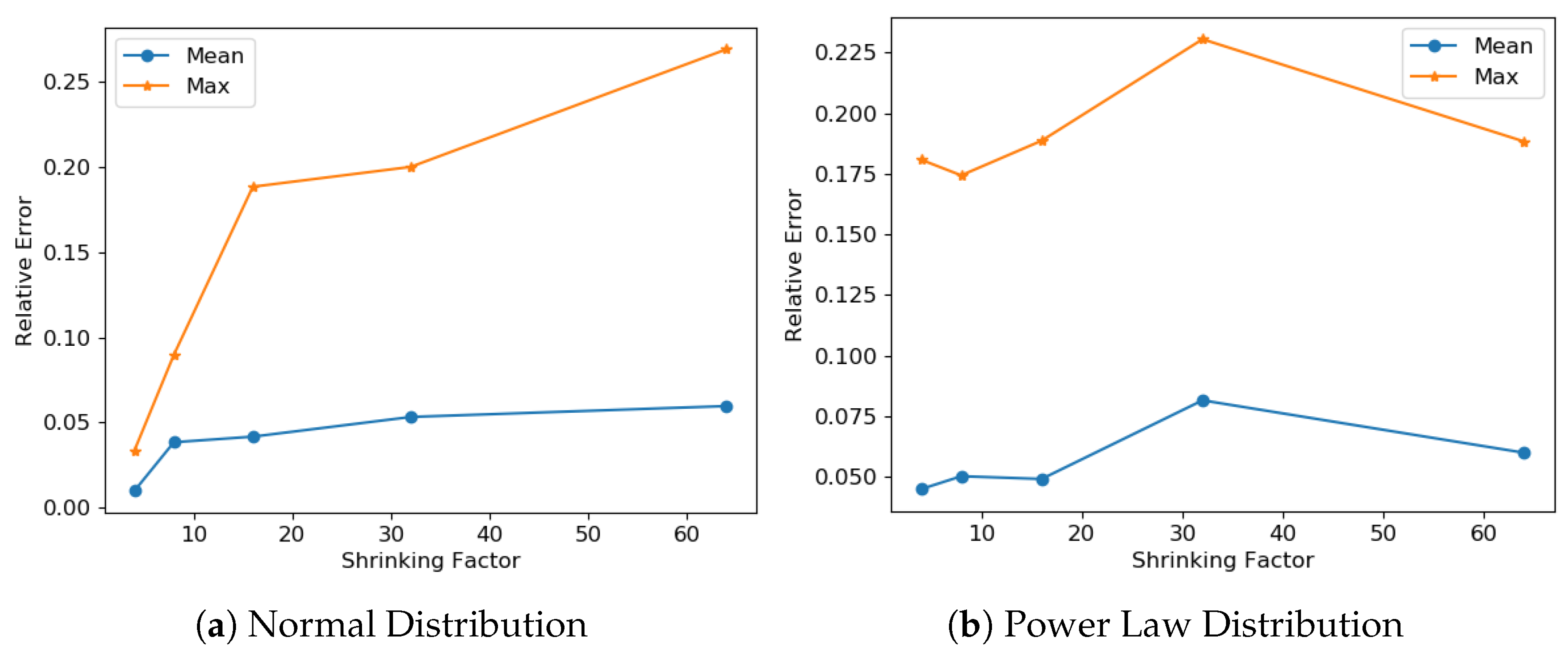
We define the shrinking factor $SF$ (a positive integer) to constrain the space allocation of a stream sketch. This means that the size of the edges and vertices of the graph sketch will be $\frac{1}{SF}$ of the original graph. The existing research on sketch building [7] shows that multiple pairwise independent hash function [4] methods can often generate better estimation results because they can reduce the probability of hash collisions. In our solution, we sample at different parts of the given sliding window instead of the complete stream and then map the sampled edges into multiple (here three) independent partitions to completely avoid collisions. We name the three partitions Head, Mid, and Tail partitions or sub-sketches, respectively. Each partition will be assigned with $\frac{1}{3SF}$ space of the original graph.

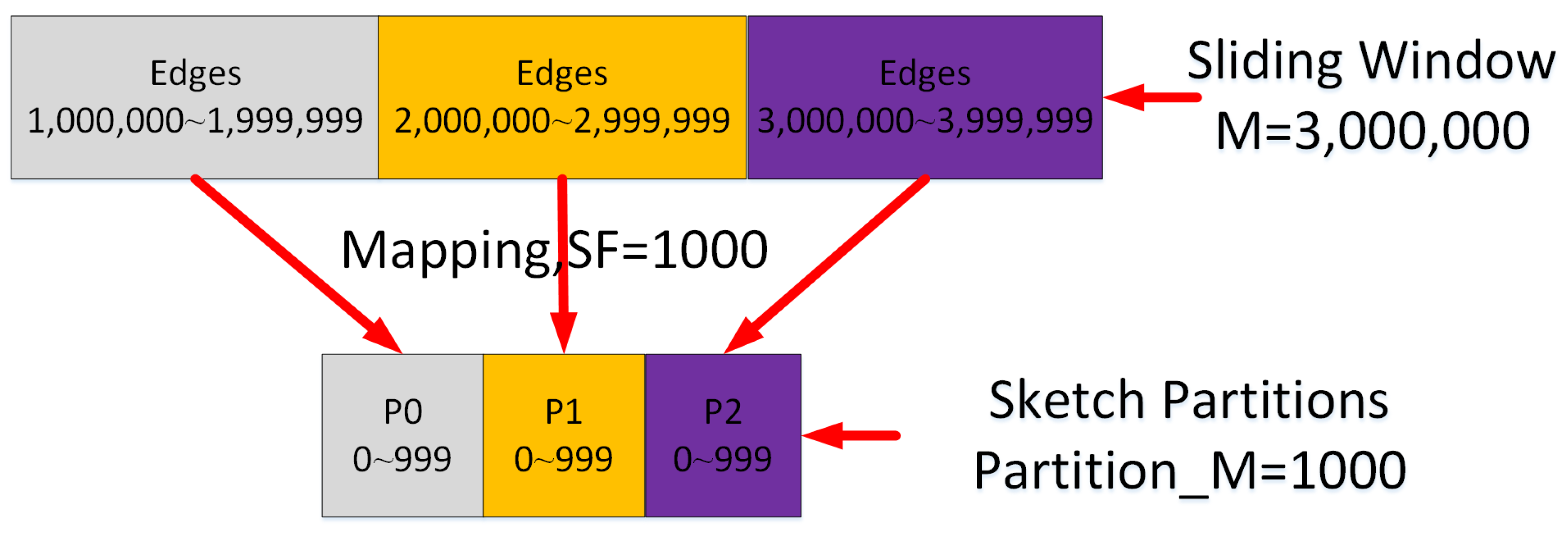
Since we divide the sketch into three independent partitions, we select a very simple hash function. For a given sliding window, we let the total number of edges and vertices in this window be M and N. Then, the size of each partition will have $Partitio{n}_M=\frac{M}{3SF}$ edges and $Partitio{n}_N=\frac{N}{3SF}$ vertices. For any edge $e=⟨i,j⟩$ from the original graph, we will map the edge ID e to $mod(e,Partitio{n}_M)$. At the same time, its two vertices i and j will be mapped to $mod(i,Partitio{n}_N)$ and $mod(j,Partitio{n}_N)$. If $e<\frac{M}{3}$, then we will map $e=⟨i,j⟩$ to the Head partition. If $e\ge \frac{2M}{3}$, we will map $e=⟨i,j⟩$ to the Tail partition. Otherwise, we will map $e=⟨i,j⟩$ to the Mid partition.

Figure 4 is an example that shows how we map, completely, 3,000,000 edges in a given sliding window into a sketch with three partitions. The edges from 1,000,000 to 1999,999 are mapped to the Head partition p0 that has 1000 edges. The edges from 2,000,000 to 2,999,999 are mapped to the Mid partition p1 and the edges from 3,000,000 to 3,999,999 are mapped to the Tail partition p2. Each partition is expressed as a graph.

Figure 4. Mapping a graph stream into a multi-partition sketch.

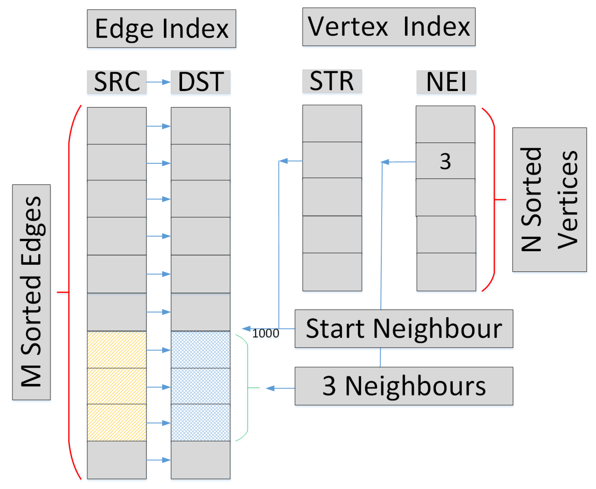
After the three smaller partitions are built, we sort the edges and create the DI data structure to store the partition graphs.

We map different parts of a stream into corresponding sub-sketches and this is very different from the existing sketch building methods. They map the same stream into different sketches with independent pairwise hash functions so each sketch is an independent summarization of the stream. However, in our method, one sub-sketch can only stand for a part of the stream and we use different sub-sketches to capture the different local features in a stream. Our regression model (see Section 5.3) will be responsible for generating the final approximate solution.

More partitions will help to capture more local features of a stream. However, we aim for a regression model that is as simple as possible. Too many partitions will make our regression model have more variables and become complicated. We select three as the default number of partitions because this can achieve sufficient accuracy based on our experimental results. Of course, for some special cases, we may choose more partitions but use the same proposed framework.

5.1.2. Insert-Only and Insert-Delete Streams

For the sliding window stream, we only need to care about the edges in the given window. However, for insert-only and insert-delete streams, we need to consider the edges that will come in the future. Here, we will describe the sketch updating mechanism in our stream model.

For the insert-delete stream, we will introduce a new weight array in the sketch. If the total number of edges that can be held in one partition is $Partitio{n}_M$, then we will introduce a weight array $E\_WEI$ with size $Partitio{n}_M$ to store the latest updated information of each edge. The initial value of $E\_WEI$ will be zero. If a new insert edge is mapped to e, then we will let $E\_WEI\left[e\right]=E\_WEI\left[e\right]+1$. If a deleted edge is mapped to e, then we will let $E\_WEI\left[e\right]=E\_WEI\left[e\right]-1$. So, for any edge in the partition, if $E\_WEI\left[e\right]=0$, it means that the edge has been deleted so we can safely remove this edge from our sketch. If $E\_WEI\left[e\right]>1$, it means that there are multiple edges in the stream that have been mapped to this edge. For the insert-only stream, it is similar to the insert-delete stream but we never reduce the value of $E\_WEI$.

To improve the sketch update performance, we will use the bulk updating mechanism for the two streams. If B new edges have arrived (they can be insert edges or delete edges), we will divide B into three parts and map them into the three different partitions just as in the method used in the sliding window stream. After the new edges are updated, we need to resort the edges and update the DI data structure to express the updated sub-sketches.

5.2. Edge–Vertex Iterator Based Triangle Counting Algorithm

We can directly employ existing exact graph algorithms in our sketch because the sketch is also expressed as a graph. Here, we will use a typical graph analysis algorithm—triangle counting—to show how we can develop optimized exact algorithms based on our $DI$ data structure.

To improve the performance of a distributed triangle counting algorithm, two important problems are maintaining load balancing and avoiding remote access or communication as much as possible.

In Chapel, the locale type refers to a unit of the machine resources on which the program is running. Locales have the capability to store variables and to run Chapel tasks. In practice, for a standard distributed memory architecture, a single multicore/SMP node is typically considered a locale. Shared memory architectures are typically considered a single locale. In this work, we will develop a multiple-locale exact triangle counting algorithm for distributed memory clusters.

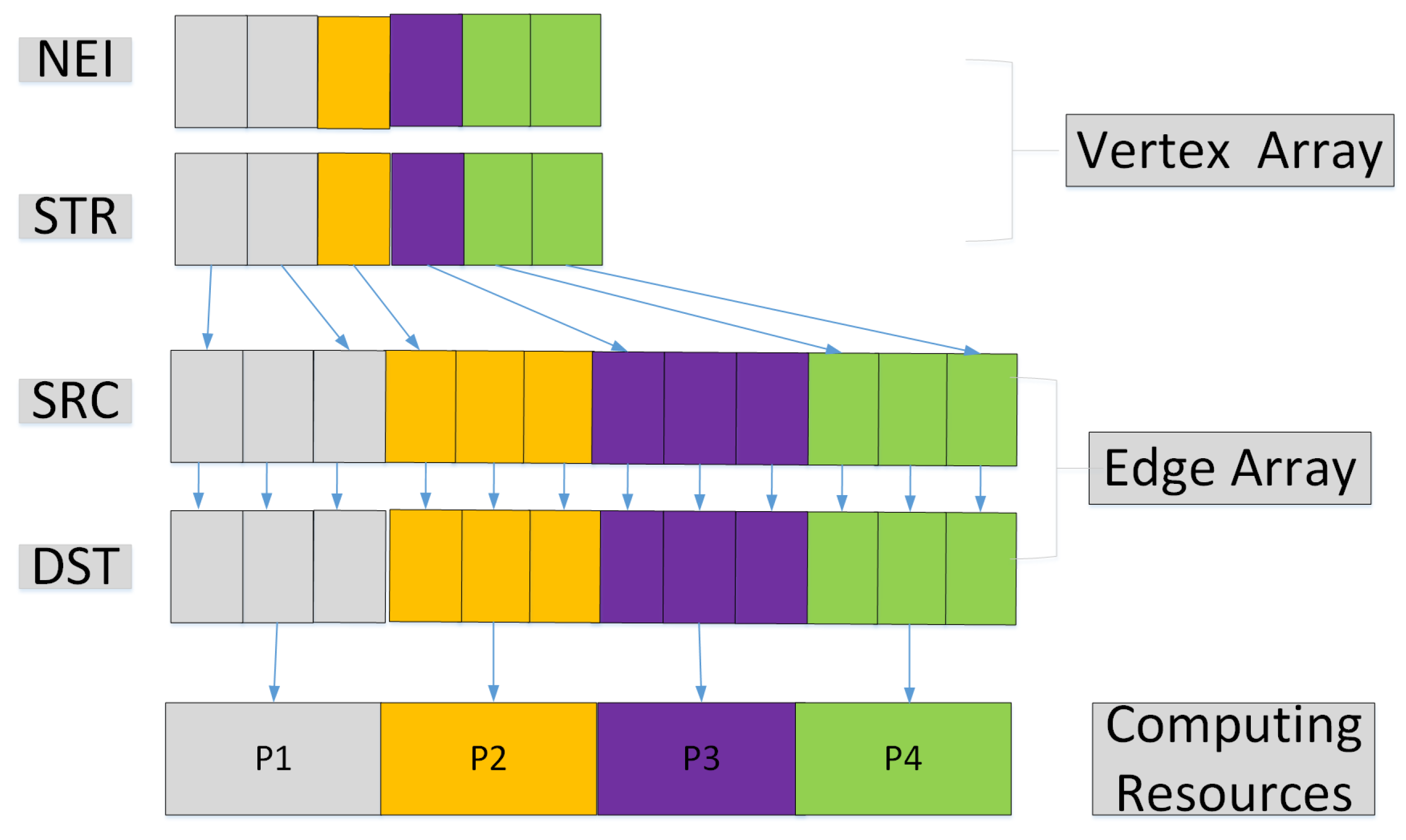
For power law graphs, a small number of vertices may have a high degree. So, if we divide the data based on number of vertices, it is easy to cause an unbalanced load. Our method divides the data based on the number of edges. At the same time, our DI data structure will keep the edges connected with the same vertex together. So, the edge partition method will result in good load balancing and data access locality.

However, if each locale directly employs the existing edge iterator [13] on its edges, the reverse edges of the undirected graphs are often not in the same locale. This will cause a new load balancing problem. So, we will first generate the vertices based on the edges distributed to different locales. Then, each locale will employ the vertex iterator to calculate the number of triangles. The combined edge–vertex iterator method is the major innovation for our triangle counting method on distributed systems.

When we employ the high level parallel language Chapel to design the parallel exact triangle counting algorithm, there are two additional advantages: (1) Our DI data structure can work together with the coforall or forall parallel construct of Chapel to exploit the parallelism; (2) We can take advantage of the high level module Set provided by Chapel to implement the parallel set operation easily and efficiently.

At a high level, our proposed algorithm takes advantage of the multi-locale feature of Chapel to handle very large graphs in distributed memory. The distributed data are processed at their locales or their local memory. Furthermore, each shared memory compute node can also process their own data in parallel. The following steps are needed to implement the multi-locale exact triangle counting algorithm: (1) The DI graph data should be distributed evenly onto the distributed memory to balance the load; (2) Each distributed node only counts the triangle including the vertices assigned to the current node; (3) All the triangles calculated by different nodes should be summed together to obtain the exact number of triangles.

Our multi-locale exact triangle counting algorithm is described in Algorithm 1. For a given graph sketch partition $G_{sk}=⟨E_{sk},V_{sk}⟩$, we will use an array $subTriSum$ to keep each locale’s result (line 2). Here in line 3, we use coforall instead of forall to allow each $loc$ in $Locales$ to execute the following code in parallel so we can fully exploit the distributed computing resources. The code between line 3 and line 17 will be executed in parallel on each locale. Each locale will use a local variable $triCount$ to store the number of triangles (line 5). Line 6 and line 7 are important for implementing load balancing. Assume edges from $e_{start}$ to $e_{end}$ are assigned to the current locale, we can obtain the corresponding vertex ID $StartVer=SRC\left[e_{start}\right]$ and $EndVer=SRC\left[e_{end}\right]$ as the vertices interval that the current locale will handle. Since different locales may have different edges with the same starting vertex, the interval $[StartVer..EndVer]$ of different locales may overlap. At the same time, some starting vertex in the $SRCr$ index array may not appear in $SRC$, so we should also make sure there is no “hole” in the complete interval $[0..|V_{sk}|-1]$. In line 7, we will make sure all the intervals will cover all the vertices without overlapping.

Our method includes the following steps: (1) If the current locale’s $StartVer$ is the same as the previous locale’s $EndVer$, this means that one vertex’s edges have been partitioned into two different locales. We will set $StartVer=StartVer+1$ to avoid two locales executing the counting on the same vertex; (2) If the current locale’s $StartVer$ is different from the previous locale’s $EndVer$, and the difference is larger than 1, this means that there is a “hole” between the last locale’s vertices and the current locale’s vertices. So we will let the current locale’s $StartVer=$ last locale’s $EndVer+1$; (3) If the current locale is the last locale, we will let its $EndVer=$ the last vertex ID. If the current locale is the first locale, we will let $StartVer=0$.

From line 8 to line 14 we will count all the triangles starting from the vertices assigned to the current locale in parallel. In line 9 we will generate all the adjacent vertices $u_{adj}$ of the current vertex u and its vertex ID is larger than u. From line 10 to line 12, for any vertex $v\in u_{adj}$, we will generate all the adjacent vertices $v_{adj}$ of current vertex v and its vertex ID is larger than v. So the number of vertices in $u_{adj}\cap v_{adj}$ is the number of triangles having edge $⟨u,v⟩$. Since we only calculate the triangles whose vertices meet $u<v<w$, we will not count the duplicate triangles. In this way, we can avoid the unnecessary calculation. In line 15, each locale will assign its total number of triangles to the corresponding position of array $subTrisum$. At the end in line 18, when we sum all the number of triangles of different locales, we will obtain the total number of triangles.

Algorithm 1: Edge–vertex Iterator triangle counting algorithm

5.3. Real-World Graph Distribution Based Regression Model

Instead of developing different specific methods for different graph analysis problems, we propose a general regression method to generate the approximate solution based on the results of different sub-sketches.

One essential objective of a stream model is generating an accurate estimation based on the query results from its sketch. The basic idea of our method is to exploit the real-world graph distribution information to build an accurate regression model. Then we can use the regression model to generate approximate solutions for different queries.

Specifically, for the triangle counting problem, when we know the exact number of triangles in each sub-sketch (see Table 1), the key problem is how we can estimate the total number of triangles.

Table 1. Sketch Triangle Number.

Graph Name	Shrinking Factor	Head	Mid	Tail	Exact
delaunay_n10	4	98	138	150	2047
delaunay_n10	8	63	72	80	2046
delaunay_n10	16	35	41	41	2044
delaunay_n10	32	20	12	16	2043
delaunay_n10	64	3	3	10	2042
delaunay_n11	4	195	302	294	4104
delaunay_n11	8	95	151	144	4103
delaunay_n11	16	62	71	63	4101
delaunay_n11	32	26	32	29	4100
delaunay_n11	64	12	24	14	4009
delaunay_n12	4	258	607	575	8215
delaunay_n12	8	163	306	293	8214
delaunay_n12	16	90	139	147	8212
delaunay_n12	32	52	78	76	8211
delaunay_n12	64	51	42	32	8210
delaunay_n13	4	646	1160	1197	16,442
delaunay_n13	8	335	598	588	16,441
delaunay_n13	16	187	297	304	16,439
delaunay_n13	32	108	144	153	16,438
delaunay_n13	64	68	62	81	16,437
delaunay_n14	4	1099	2356	2299	32,921
delaunay_n14	8	507	1205	1184	32,920
delaunay_n14	16	269	568	579	32,918
delaunay_n14	32	135	294	303	32,917
delaunay_n14	64	93	144	137	32,916
delaunay_n15	4	2085	4571	4585	65,872
delaunay_n15	8	943	2335	2320	65,871
delaunay_n15	16	486	1140	1159	65,869
delaunay_n15	32	265	568	580	65,868
delaunay_n15	64	137	282	299	65,867
delaunay_n16	4	4168	9648	9510	131,842
delaunay_n16	8	2170	4666	4601	131,841
delaunay_n16	16	1063	2387	2348	131,839
delaunay_n16	32	569	1174	1169	131,838
delaunay_n16	64	326	576	580	131,837
delaunay_n17	4	8154	18,873	18,938	263,620
delaunay_n17	8	4012	9543	9501	263,619
delaunay_n17	16	2132	4595	4773	263,617
delaunay_n17	32	1042	2288	2347	263,616
delaunay_n17	64	534	1156	1180	263,615
delaunay_n18	4	16,904	37,774	38,061	527,234
delaunay_n18	8	8155	19,005	19,107	527,233
delaunay_n18	16	4176	9454	9562	527,231
delaunay_n18	32	2097	4674	4686	527,230
delaunay_n18	64	1004	2369	2348	527,229
amazon	4	4944	6383	18,381	667,259
amazon	8	1427	1752	7351	667,258
amazon	16	621	617	3614	667,256
amazon	32	331	290	2250	667,255
amazon	64	177	153	1546	667,254
dblp	4	20,269	41,390	168,996	2,225,882
dblp	8	6876	17,043	67,782	2,225,881
dblp	16	2684	4846	20,310	2,225,879
dblp	32	1097	2726	11,456	2,225,878
dblp	64	545	2325	2678	2,225,877
ca-HepTh.txt	4	1267	1072	3853	28,677
ca-HepTh.txt	8	642	591	1741	28,676
ca-HepTh.txt	16	456	390	480	28,674
ca-HepTh.txt	32	391	267	219	28,673
ca-HepTh.txt	64	260	217	157	28,672
ca-CondMat.txt	4	7960	10,280	12,051	174,578
ca-CondMat.txt	8	4264	4970	5543	174,577
ca-CondMat.txt	16	2862	2847	2655	174,575
ca-CondMat.txt	32	1888	1693	1403	174,574
ca-CondMat.txt	64	1179	1292	845	174,573
ca-AstroPh.txt	4	75,594	78,234	78,855	1,374,119
ca-AstroPh.txt	8	41,331	47,387	40,395	1,374,118
ca-AstroPh.txt	16	24,828	28,244	20,468	1,374,116
ca-AstroPh.txt	32	14,984	16,692	11,128	1,374,115
ca-AstroPh.txt	64	6450	6507	6322	1,374,114
email-Enron.txt	4	70,077	28,783	25,933	727,044
email-Enron.txt	8	22,331	13,593	15,197	727,043
email-Enron.txt	16	11,640	8381	5002	727,041
email-Enron.txt	32	6681	5212	2392	727,040
email-Enron.txt	64	3561	2912	1056	727,039
ca-GrQc.txt	4	1193	3374	5300	48,265
ca-GrQc.txt	8	671	2131	1096	48,264
ca-GrQc.txt	16	346	880	733	48,262
ca-GrQc.txt	32	276	694	385	48,261
ca-GrQc.txt	64	64	221	150	48,260
ca-HepPh.txt	4	118,540	74,598	187,003	3,345,241
ca-HepPh.txt	8	44,937	33,404	64,281	3,345,240
ca-HepPh.txt	16	16,775	16,426	35,817	3,345,238
ca-HepPh.txt	32	3708	6643	8724	3,345,237
ca-HepPh.txt	64	705	3707	2899	3,345,236
loc-brightKite_edges.txt	4	12,232	4435	2489	301,812
loc-brightKite_edges.txt	8	5266	3217	1652	301,811
loc-brightKite_edges.txt	16	2579	1673	927	301,809
loc-brightKite_edges.txt	32	1061	1335	380	301,808
loc-brightKite_edges.txt	64	552	856	280	301,807

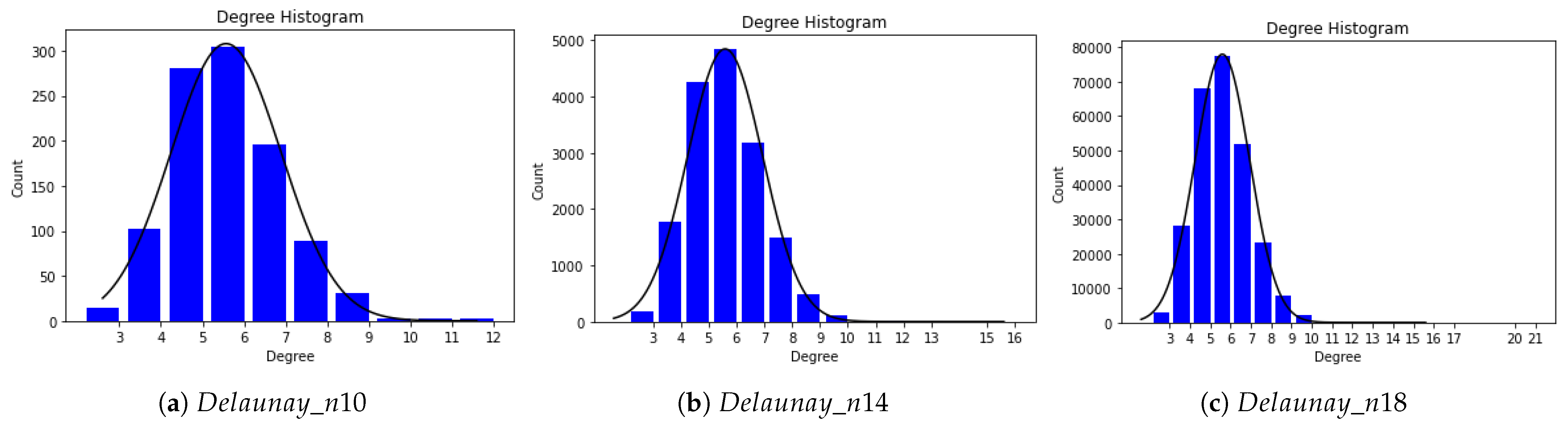
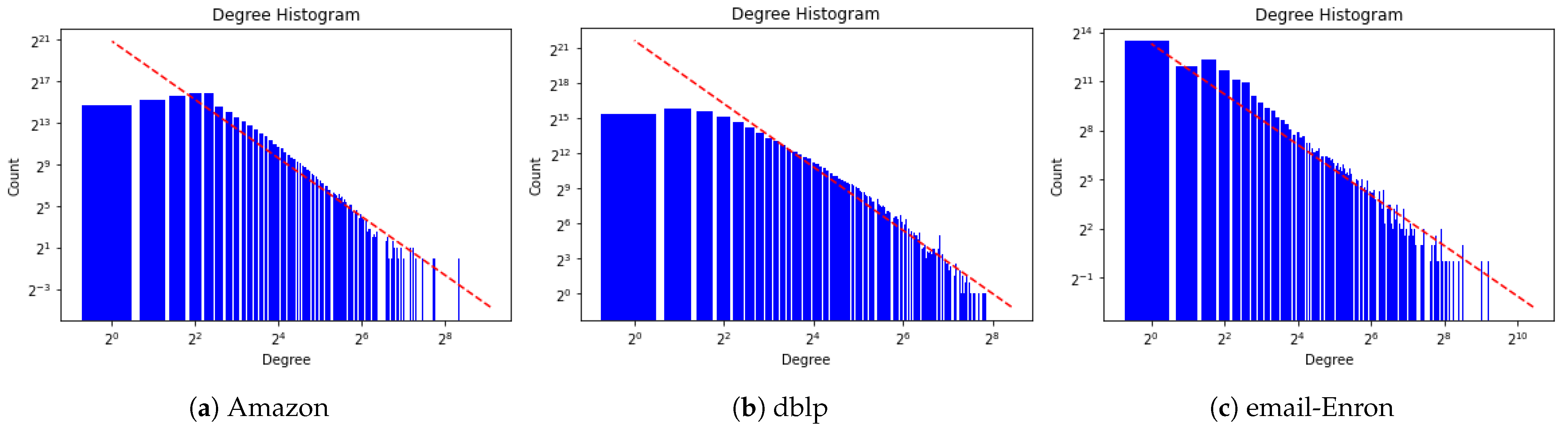
To achieve user-required accuracy for different real-world applications, our method exploits the features of real-world graph distributions. Many sparse networks—social networks in particular—have an important property; their degree distribution follows the power law distribution. Normal distributions are often used in the natural and social sciences to represent real-valued random variables whose distributions are not known. So, we develop two regression models for the two different graph degree distributions.

We let $E_H,E_M,E_T$ be the exact number of triangles in the Head, Mid and Tail sub-sketches. The exact triangle counting algorithm is given in Section 5.2.

For normal degree distribution graphs, we assume that the total number of triangles has a linear relationship with the number of triangles in each sub-sketch. We take $E_H,E_M,E_T$ as three randomly sampled results of the original stream graph to build our multivariate linear regression model. $T{C}_{Normal}$ is the estimated number of triangles and the regression model is given in Equation (1).

$$T{C}_{Normal}=a\times E_H+b\times E_M+c\times E_T.$$

(1)

For power law graphs, the sampling results of $E_H,E_M,E_T$ can be significantly different because of the skewness in degree distribution. A power law distribution has the property that its log–log plot is a straight line. So we assume the logarithmic value of the total number of triangles in a stream graph should have a linear relationship with the logarithmic values of the exact number of triangles in different degree sub-sketches. Then we have two ways to build the regression model. One is unordered and the other is ordered. The unordered model can be expressed as in Equation (2). In this model, the relative order information of sampling results cannot be captured.

$$T{C}_{powerlaw,log}=a\times E_{H,log}+b\times E_{M,log}+c\times E_{T,log},$$

(2)

where $T{C}_{powerlaw,log}=log\left(T{C}_{powerlaw}\right)$ is the logarithmic value of the estimated value $T{C}_{powerlaw}$; $E_{H,log}=log\left(E_H\right),$$E_{M,log}=log\left(E_M\right),$ and $E_{T,log}=log\left(E_T\right)$; $log\left(E_H\right),$$log\left(E_M\right),$ and $log\left(E_T\right)$ are the logarithmic values of $E_H,E_M,$ and $E_T$, respectively.

Then, we refine the regression model for power law distribution as follows. We get $E_{min},E_{median}$ and $E_{max}$ by sorting $E_H,E_M,$ and $E_T$. They mean the minimum, median and maximum sampling values of the number of triangles. They will be used to stand for the sampling results of a power law distribution at the right (low possibility), middle (a little bit high possibility) and left part (very high possibility). We let $E_{min,log}=log\left(E_{min}\right),$$E_{median,log}=log\left(E_{median}\right),$ and $E_{max,log}=log\left(E_{max}\right)$. Our ordered multivariate linear regression model for power law graphs is given in Equation (3).

$$T{C}_{powerlaw,log}=a\times E_{min,log}+b\times E_{median,log}+c\times E_{max,log}.$$

(3)

The accuracy of our multivariate linear regression model is given in in Section 7.3.1 and we can see that the ordered regression model is better than the unordered regression model. Both of our normal and ordered power law regression models achieve a very high accuracy.

6. Integration with Arkouda

Based on the current Arkouda framework, the communication mechanism can be directly reused between Python and Chapel. To support large graph analysis in Arkouda, the major work is implementing the graph data structure and the corresponding analysis functions in both Python and the Chapel package. In this section, we will introduce how we define the graph classes to implement our DI data structure and develop a corresponding Python benchmark to drive the triangle counting method.

6.1. Graph Classes Definition in Python and Chapel

Our DI data structure can also support graph weight. If each vertex has a different weight, we use an array $V\_WEI$ to express the weight values. If each edge has a weight, we use an array $E\_WEI$ to stand for different weights. Based on our DI data structure, four class directed graph (GraphD), directed and weighted graph (GraphDW), undirected graph (GraphUD) and undirected and weighted graph (GraphUDW) are defined in Python. Four corresponding classes—SegGraphD, SegGrapDW, SegGraphUD, SegGraphUDW—are also defined in Chapel to present different kinds of graphs. In our class definition, directed graph is the base class. Then, undirected graph and directed and weighted graph are the two child classes. Finally, undirected and weighted graph will inherit from undirected graph.

All the graph classes, including their major attributes, are given in Table 2. The left columns are the Python classes and their descriptions. The right columns are the corresponding Chapel classes and their descriptions. Based on the graph class definition, we can develop different graph algorithms.

Table 2. Double-Index Sparse Graph Class Definition in Python and Chapel.

Python		Chapel
Class	Attribute and Description	Class	Attribute and Description
GraphD	n_vertices: number of vertices	SegGraphD	$n\_vertices$: number of vertices
	$n\_edges$: number of edges		$n\_edges$: number of edges
	$directed$: directed graph or not		$directed$: directed graph or not
	$weighted$: weighted graph or not		$weighted$: weighted graph or not
	$src$: the source of every edge in the graph		$srcName/src$: the name and data of source array
	$dst$: the destination of every edge in the graph		$dstName/dst$: the name and data instance of the destination array
	$start\_i$: starting index of all the vertices in $src$		$startName/start\_i$: the name and data instance of the starting index array
	$neighbor$: number of neighbors all the vertices		$neighborName/neighbor$: the name and data instance of the neighbor array
GraphDW(GraphD)	$v\_weight$: weight of vertex	SegGraphDW:SegGraphD	$v\_weightName/v\_weight$: name and data instance of the vertex weight array
	$e\_weight$: weight of edge		$e\_weightName/e\_weight$: name and data instance of the edge array
GraphUD(GraphD)	$srcR$: the source of every reverse edge in the graph	SegGraphUD:SegGraphD	$srcNameR/srcR$: name and data instance of the reverse source array
	$dstR$: the destination of every reverse edge in the graph		$dstNameR/dstR$: the name and data instance of the reverse destination array
	$start\_iR$: starting index of all the vertices in reverse $src$		$startNameR/star{t}_{i}R$: the name and data of the reverse starting index array
	$neighborR$: number of neighbors all the vertices in $srcR$		$neighborNameR$: the name and data of the reverse neighbor array
GraphUDW(GraphUD)	$v\_weight$: weight of vertex	SegGraphUDW:SegGraphUD	$v\_weightName/v\_weight$: the name and data of the vertex weight array
	$e\_weight$: weight of edge		$e\_weightName$: the name and data of the edge array

6.2. Triangle Counting Benchmark

To compare the performance of the exact method and our approximate method, we implement two triangle counting related functions. For the exact method, we implement the “graph_file_read” and “graph_triangle” Python functions to read a complete graph file and call our triangle counting kernel algorithm (Algorithm 1) to calculate the number of triangles.

For our approximate method, we implement the “stream_file_read” function to simulate the stream by reading a graph file’s edges one by one. The graph sketch introduced in Section 5.1 will be built automatically when we read the edges. Currently, we only implement the sliding window streaming’s sketch building. Automatically building the insert-only and insert-delete streaming will be future work after we evaluate our data structure and sketch with a larger collection of graph algorithms.

After the sketch of a sliding window stream is built in the memory, we will call on the “stream_tri_cnt” function to first calculate the exact number of triangles in each sub-sketch (it will also call on our kernel triangle counting Algorithm 1) and then use the regression model to estimate the total number of triangles in the given stream.

For the power law distribution regression model, in the benchmark we also implement single variable regression models using the maximum, minimum and median results of the three sub-sketches respectively. Our testing results show that the proposed regression method in Section 5.3 can achieve a better accuracy.

7. Experiments

7.1. Experimental Setup

Testing of the methods was conducted in an environment composed of a 32 node cluster with an FDR Infiniband between the nodes in the cluster. Infiniband connections between nodes is commonly found in high performance computers. Every node is made up of 512 GB of RAM and two 10-core Intel Xeon E5-2650 v3 @ 2.30 GHz processors with 20 cores total. Due to Arkouda being designed primarily for data analysis in an HPC setting, an architecture setup that aptly fits an HPC scenario was chosen for testing.

7.2. Datasets Description and Analysis

We will use graph files and read the edges line by line to simulate the sliding window of a graph stream. The graphs selected for testing were chosen from various publicly available datasets for the benchmarking of graph methods. These include datasets from the 10th DIMACS Implementation Challenge [40], as well as some real-life graph datasets from the Stanford Network Analysis Project (SNAP) http://snap.stanford.edu/data/ (accessed on 20 July 2021). Pertinent information about these datasets for the triangle counting method are displayed in Table 3.

Table 3. Graph benchmarks utilized for the triangle counting algorithm.

Degree Distribution	Graph Name	Edges	Vertices	Mean	Standard Deviation
Normal	delaunay_n10	3056	1024	5.96875	3.10021
	delaunay_n11	6127	2048	5.98340	3.76799
	delaunay_n12	12,264	4096	5.98828	3.49865
	delaunay_n13	24,547	8192	5.99292	3.25055
	delaunay_n14	49,122	16,384	5.99634	3.30372
	delaunay_n15	98,274	32,768	5.99817	3.37514
	delaunay_n16	196,575	65,536	5.99899	3.35309
	delaunay_n17	393,176	131,072	5.99938	3.26819
	delaunay_n18	786,396	262,144	5.99972	3.2349
Degree Distribution	Graph Name	Edges	Vertices	a	k
power law	amazon	925,872	334,863	1,920,877	2.81
	dblp	1,049,866	317,080	3,299,616.65	2.71
	youtube	2,987,624	1,134,890	701,179.83	1.58
	lj	34,681,189	3,997,962	50,942,065.49	2.40
	orkut	117,185,083	3,072,441	40,351,890.91	2.12
	ca-HepTh	51,971	9877	23,538.9	2.29
	ca-CondMat	186,936	23,133	68,923.6	2.23
	ca-AstroPh	396,160	18,772	46,698.3	1.84
	email-Enron	367,662	36,692	10,150.2	1.54
	ca-GrQc	28,980	5242	6610.35	2.04
	ca-HepPh	237,010	12,008	4601.72	1.44
	loc-brightkite_edges	214,078	58,228	44,973.1	1.88

Based on the graphs’ degree distribution, we divided them into two classes, normal distribution and power law distribution. Prior research has shown that some real-world graphs follow power law distributions. Normal distributions are also found ubiquitously in the natural and social sciences to represent real-valued random variables whose distributions are not known. For normal distributions, their typical parameters, the mean and standard deviation fitted from the given graphs, are listed in Table 3 too. Figure 5 shows the comparison between the fitting results and the original graph data. We can see that the fitting results can match with the original data very well. In other words, the Delaunay graphs follow the normal distribution.

Figure 5. Normal distribution graphs.

For graphs that follow the power law distribution $y\left(x\right)=a\times x^{-k}$, we also present their fitting parameters a and k in Table 3. Figure 6 provides some examples of these graphs. We can see that, in general, their signatures are close to power laws. However, we can also see that some data do not fit a power law distribution very well.

Figure 6. Power law distribution graphs.

7.3. Experimental Results

7.3.1. Accuracy

In order to evaluate the accuracy of our method, we conducted experiments on nine normal distribution and 12 power law distribution benchmark graphs with shrink factors 4, 8, 16, 32, and 64. In total, we have 105 test cases. For each test, we will have three triangle numbers for the Head, Mid and Tail sketch partitions. We will use the exact number of triangles in the three sub-sketches to provide the approximate number of triangles in the given graph stream. The testing results are given in Table 1.

For the normal distribution, based on our regression model expressed as Equation (1), we can get the parameters and express the multivariate linear regression equation as:

$$T{C}_{Normal}=0.7264\times E_H+1.4157\times E_M+1.7529\times E_T.$$

When we compute the absolute value of all the percent error, the mean error is 4%, the max error is 25% and the R-squared value is 1, and this means that the sketch results are absolutely related to the final number of triangles.

We also evaluated our regression model to see how the accuracy changes with the shrinking factor. For a normal distribution, we built five regression models by selecting the shrinking factors as 4, 8, 16, 32, and 64, respectively. The result is shown in Figure 7. We can see that both the mean and max error will increase when we doubly increase the value of the shrinking factor step by step. However, the mean increases very slowly. The mean error changes from 1% to 5.97%. The max error will increase from 3.36% to 26.87%. This result shows that our regression model for normal distribution graphs is stable and very accurate. When the graph size shrinks to half of its previous size, there is a very small effect on the accuracy when the number of triangles is not less than some threshold value. This is important because we can use much smaller sketches to achieve very accurate results.

Figure 7. How accuracy changes with shrinking factor for normal and power law distribution graphs.

For the power law distribution, based on our ordered regression model in Equation (3) which is refined from the unordered regression model, the log value multivariate linear regression equation can be expressed as:

$$T{C}_{powerlaw,log}=-0.4464\times E_{min,log}+0.1181\times E_{median,log}+1.4236\times E_{max,log}.$$

The mean error is 3.2%. The max value is 7.2%. The R-squared value is 0.91. This means that the model can describe the data very well. If we use the unordered regression model, Equation (2), the mean error is 4.5%. The max value is 12.5%. R-squared is 0.81. All the results are worse than the results of the ordered regression model in Equation (3).

We also performed experiments to show the accuracy of ordered and unordered regression models when we built five different regression models using different shrinking factors of 4, 8, 16, 32, and 64. The experimental results are presented in Table 4 and we can make two conclusions from the results: (1) All the results of our ordered regression model are better than the results of the unordered regression model. This means that when we exploit more degree distribution information and integrate it into our model, we can achieve a better accuracy; (2) When we double the value of the shrinking factor, the change in accuracy is much smaller than the change in the normal regression model. This also means that, in the power law model, the accuracy is much less sensitive to the shrinking factor because the power law graph is highly skewed. This conclusion also means that we can use a relatively smaller shrinking factor to achieve almost the same accuracy.

Table 4. Comparison between Ordered and Unordered Regression Models for Power Law Distribution.

Metrics		AbsMaxError		AbsMeanError		R-Squared
Regression Methods		Ordered	Unordered	Ordered	Unordered	Ordered	Unordered
Shrink Factor	4	6.76%	8.26%	2.84%	3.75%	91.42%	85.10 %
	8	6.08%	8.89%	3.05%	4.13%	91.59%	82.90%
	16	4.16%	8.66%	1.97%	3.64%	96.47%	87.85%
	32	6.67%	10.80%	3.02%	4.02%	90.85%	82.73%
	64	4.66%	6.68%	2.86%	3.02%	94.12%	92.04%

The accuracy evaluation results show that the proposed regression model for normal distribution graphs and power law distribution graphs can achieve very accurate results. For both, the mean relative error is less than 4%. However, if we employ the normal regression model in Equation (1) to the power-law distribution data, the mean relative error can be as high as 26%, and the max relative error is 188%. This means that employing different regression models for different degree distribution graphs may significantly improve the accuracy.

7.3.2. Performance

Existing exact triangle counting algorithms show that, for very large graphs, the communication between different computing nodes will consume the majority of the time. Therefore, reducing the total communication, or improving data access locality during triangle counting, are the key factors for improving the final performance.

Since our triangle counting method can maintain load balancing and locality, it can achieve a high performance for large graph streams. Our experimental results show that our streaming triangle algorithm displays high locality. These results are provided in Table 5. We calculate all the local data access times and all the remote data access times during the triangle counting procedure. We define the locality access ratio $LAR=\frac{NL}{NL+NR}$, where $NL$ is the total number of local accesses and $NR$ is the total number of remote accesses. For the three sub-sketches—Head, Mid and Tail—we calculate their LAR values, respectively. From the table we can see that, for all cases, the LAR value is larger than 50% and the average LAR value is 74%. This means that, during our triangle counting procedure, most of the data come from local memory. This is the major reason our method can achieve a high performance.

Table 5. Local Access Ratio of different stream graphs.

Filename	Head Local Access Ratio	Mid Local Access Ratio	Tail Local Access Ratio
delaunay_n10	0.736364	0.75	0.642045
delaunay_n11	0.578635	0.789894	0.707775
delaunay_n12	0.737226	0.906832	0.878136
delaunay_n13	0.710651	0.902913	0.91839
delaunay_n14	0.661084	0.914058	0.941802
delaunay_n15	0.699193	0.963969	0.947161
delaunay_n16	0.685931	0.968672	0.953034
delaunay_n17	0.692844	0.972879	0.963517
delaunay_n18	0.693935	0.983028	0.975103
ca-HepTh.txt	0.687343	0.645873	0.650115
ca-CondMat.txt	0.630154	0.663701	0.6764
ca-AstroPh.txt	0.61735	0.615687	0.615749
email-Enron.txt	0.376773	0.632443	0.785357
ca-GrQc.txt	0.721421	0.671429	0.687907
ca-HepPh.txt	0.643376	0.648718	0.593803
loc-brightkite_edges.txt	0.71338	0.603389	0.721972
amazon	0.731695	0.723097	0.738042
dblp	0.605114	0.711748	0.830386
youtube	0.669736	0.671671	0.9342
lj	0.570621	0.728383	0.993926
orkut	0.556868	0.569822	0.861902

To show the speedup of the streaming process, we compare the execution time of the original complete graph triangle counting and the execution time of our sketch method. The experimental results are given in Table 6. From the table we can see that our streaming method uses much less space and runs much faster to estimate the number of triangles in large graph stream with only one pass. Since the experimental time is very long for large graphs, here we just present three different shrinking factors to show the trend. We can see that, for very large graphs, we can use a very large shrinking factor to significantly reduce the processing space, and the absolute speedup is also very high. However, the relative speedup compared with the shrinking factor is a little bit lower. For relatively small graphs, our shrinking factor is also relatively small, so the absolute speedup is also small but the relative speedup is high. Our experimental results show that the speedup will increase almost linearly with the shrinking factor.

Table 6. Speedup of Stream graph processing.

Graph Name	Factor	Stream Time (s)	Exact Time (s)	Speedup
delaunay_n12	4	2.04689	2.72048	1.33
delaunay_n12	8	1.8969	2.72048	1.43
delaunay_n12	16	1.77604	2.72048	1.53
delaunay_n13	4	2.67814	4.70596	1.76
delaunay_n13	8	2.27257	4.70596	2.07
delaunay_n13	16	2.0258	4.70596	2.32
delaunay_n14	4	3.94324	8.91793	2.26
delaunay_n14	8	3.04275	8.91793	2.93
delaunay_n14	16	2.60059	8.91793	3.43
delaunay_n15	4	6.34795	17.4302	2.75
delaunay_n15	8	4.44783	17.4302	3.92
delaunay_n15	16	3.6619	17.4302	4.76
delaunay_n16	4	11.2135	34.2433	3.05
delaunay_n16	8	7.29339	34.2433	4.70
delaunay_n16	16	5.65829	34.2433	6.05
delaunay_n17	4	21.0084	68.4882	3.26
delaunay_n17	8	13.0833	68.4882	5.23
delaunay_n17	16	9.71683	68.4882	7.05
delaunay_n18	4	40.4338	135.191	3.34
delaunay_n18	8	24.8456	135.191	5.44
delaunay_n18	16	17.8642	135.191	7.57
delaunay_n18	32	14.1647	135.191	9.54
delaunay_n18	64	12.0415	135.191	11.23
delaunay_n19	32	26.6216	270.491	10.16
delaunay_n19	64	22.5967	270.491	11.97
delaunay_n19	128	20.9203	270.491	12.93
delaunay_n20	32	51.7499	536.331	10.36
delaunay_n20	64	44.3933	536.331	12.08
delaunay_n20	128	40.2489	536.331	13.33
delaunay_n21	32	104.236	1076.77	10.33
delaunay_n21	64	87.0196	1076.77	12.37
delaunay_n21	128	80.7149	1076.77	13.34
delaunay_n22	32	208.478	2155.85	10.34
delaunay_n22	64	177.637	2155.85	12.14
delaunay_n22	128	158.13	2155.85	13.63
delaunay_n23	64	352.531	4356.982	12.36
delaunay_n23	128	317.053	4356.982	13.74
delaunay_n23	256	301.295	4356.982	14.46
delaunay_n24	128	645.002	8708.3756	13.50
delaunay_n24	256	604.981	8708.3756	14.39
delaunay_n24	512	598.49	8708.3756	14.55
amazon	16	20.4202	147.926	7.24
amazon	32	16.2884	147.926	9.08
amazon	64	14.0285	147.926	10.54
ca-AstroPh	4	16.1657	33.1578	2.05
ca-AstroPh	8	11.0193	33.1578	3.01
ca-AstroPh	16	8.38061	33.1578	3.96
ca-CondMat	4	8.70114	16.5758	1.91
ca-CondMat	8	6.20076	16.5758	2.67
ca-CondMat	16	4.86599	16.5758	3.41
ca-GrQc	4	2.65749	3.23613	1.22
ca-GrQc	8	2.20744	3.23613	1.47
ca-GrQc	16	2.02119	3.23613	1.60
ca-HepPh	4	10.263	21.3077	2.08
ca-HepPh	8	6.98969	21.3077	3.05
ca-HepPh	16	5.45666	21.3077	3.90
ca-HepPh	32	4.83524	21.3077	4.41
ca-HepPh	64	4.3246	21.3077	4.93
ca-HepTh	4	3.78554	5.37471	1.42
ca-HepTh	8	2.92663	5.37471	1.84
ca-HepTh	16	2.46299	5.37471	2.18
dblp	16	22.0434	163.092	7.40
dblp	32	17.8394	163.092	9.14
dblp	64	15.4684	163.092	10.54
email-Enron	4	16.133	63.1888	3.92
email-Enron	8	10.859	63.1888	5.82
email-Enron	16	8.04875	63.1888	7.85
lj	512	409.672	6937.4	16.93
lj	1024	393.518	6937.4	17.63
lj	2048	397.583	6937.4	17.45
loc-brightkite_edges	4	14.1111	30.1892	2.14
loc-brightkite_edges	8	10.1597	30.1892	2.97
loc-brightkite_edges	16	8.09854	30.1892	3.73
youtube	512	36.2397	951.094	26.24
youtube	1024	34.9246	951.094	27.23
youtube	2048	34.6978	951.094	27.41

We also use an even larger graph benchmark, com-Friendster, a network dataset that has 1,806,067,135 edges and 65,608,366 vertices https://snap.stanford.edu/data/ (accessed on 20 July 2021), and run it with two locales. When the shrinking factor is 32,768, it will take 44,719.4 s to build the sketch with a maximum of 235,332KB memory footprint. The triangle counting time is 22,368.2 s. When the shrinking factor is 65,536, it will take 44,593.0 s to build the sketch with a maximum of 235,288KB memory footprint. The triangle counting time is 22,296.0 s. If we use the exact method, also with two locales, the program will fail because it runs out of memory. This example really shows that our method can handle very large graphs in a limited memory footprint.

8. Conclusions

Interactive graph stream analysis is a challenging problem. In this paper, we present our solution to show how we can solve the problem in the open source framework Arkouda. The advantage of Arkouda lies in two aspects: high productivity and high performance. High productivity means that the end users can use a popular data science language such as Python to explore different graph streams. High performance means that the end users can break the limit of their laptop and personal computer’s capabilities in memory and calculation to handle very large graphs in an interactive way.

We design a double index data structure to support quick search from a given vertex to edges or from a given edge to vertices. This greatly reduces the total memory footprint for large sparse graph streams. Based on the proposed double index data structure, we develop an efficient multiple-partition stream sketch building method. Our sketch can support general stream query problems because our sketch uses a small graph to summarize a large graph. We define a shrinking factor to let users control the size of final sketch accurately. We exploit the ubiquitous normal and power law degree distributions of given graph streams to propose two regression models to estimate the results of the graph streams from their sketch partitions. Based on the double index data structure, we develop a multi-locale distributed triangle counting algorithm that can maintain load balancing and a high local data access ratio to improve the graph stream processing performance. All our methods have been integrated into the Arkouda framework and users can use a Jupyter Notebook to drive the interactive graph stream analytics pipeline easily.

Experimental results on two kinds of large sparse graph streams—normal distribution and power law distribution—show that the proposed method can achieve very high approximate results with a mean error no larger than 4%. The average local access ratio is 74% and the graph stream processing speedup increases almost linearly with the shrinking factor. This work shows that Arkouda is a promising framework for supporting large scale interactive graph stream analytics. Of course, the reported work is just the first step in supporting a typical graph query, triangle counting. In future work, we will provide more graph stream algorithms based on our sketch methodology and will further optimize the performance of our algorithms in Arkouda.

References

1. McGregor, A. Graph stream algorithms: A survey. ACM Sigmod Rec. 2014, 43, 9–20. [Google Scholar] [CrossRef]
2. Alon, N.; Matias, Y.; Szegedy, M. The space complexity of approximating the frequency moments. J. Comput. Syst. Sci. 1999, 58, 137–147. [Google Scholar] [CrossRef]
3. Manku, G.S.; Motwani, R. Approximate frequency counts over data streams. In VLDB’02: Proceedings of the 28th International Conference on Very Large Databases; Elsevier: Amsterdam, The Netherlands, 2002; pp. 346–357. [Google Scholar]
4. Cormode, G.; Muthukrishnan, S. An improved data stream summary: The count-min sketch and its applications. J. Algorithms 2005, 55, 58–75. [Google Scholar] [CrossRef]
5. Cohen, E.; Kaplan, H. Tighter estimation using bottom k sketches. Proc. VLDB Endow. 2008, 1, 213–224. [Google Scholar] [CrossRef][Green Version]
6. Zhao, P.; Aggarwal, C.C.; Wang, M. gSketch: On query estimation in graph streams. arXiv 2011, arXiv:1111.7167. [Google Scholar] [CrossRef]
7. Tang, N.; Chen, Q.; Mitra, P. Graph stream summarization: From big bang to big crunch. In Proceedings of the 2016 International Conference on Management of Data (SIGMOD), San Francisco, CA, USA, 26 June–1 July 2016; pp. 1481–1496. [Google Scholar]
8. Behrens, J.T. Principles and procedures of exploratory data analysis. Psychol. Methods 1997, 2, 131. [Google Scholar] [CrossRef]
9. Good, I.J. The philosophy of exploratory data analysis. Philos. Sci. 1983, 50, 283–295. [Google Scholar] [CrossRef]
10. Jebb, A.T.; Parrigon, S.; Woo, S.E. Exploratory data analysis as a foundation of inductive research. Hum. Resour. Manag. Rev. 2017, 27, 265–276. [Google Scholar] [CrossRef]
11. Merrill, M.; Reus, W.; Neumann, T. Arkouda: Interactive data exploration backed by Chapel. In Proceedings of the ACM SIGPLAN 6th on Chapel Implementers and Users Workshop (CHIUW), Phoenix, AZ, USA, 22 June 2019; p. 28. [Google Scholar]
12. Reus, W. CHIUW 2020 Keynote: Arkouda: Chapel-Powered, Interactive Supercomputing for Data Science. In Proceedings of the Chapel Implementers and Users Workshop (CHIUW), 2020 IEEE International Parallel and Distributed Processing Symposium Workshops (IPDPSW), Online, 22 May 2020; p. 650. [Google Scholar]
13. Al Hasan, M.; Dave, V.S. Triangle counting in large networks: A review. Wiley Interdiscip. Rev. Data Min. Knowl. Discov. 2018, 8, e1226. [Google Scholar] [CrossRef]
14. Dhulipala, L.; Blelloch, G.E.; Shun, J. Low-latency graph streaming using compressed purely-functional trees. In Proceedings of the 40th ACM SIGPLAN Conference on Programming Language Design and Implementation (PLDI), Phoenix, AZ, USA, 22–26 June 2019; pp. 918–934. [Google Scholar]
15. Macko, P.; Marathe, V.J.; Margo, D.W.; Seltzer, M.I. Llama: Efficient graph analytics using large multiversioned arrays. In Proceedings of the 2015 IEEE 31st International Conference on Data Engineering (ICDE), Seoul, South Korea, 13–17 April 2015; pp. 363–374. [Google Scholar]
16. Kumar, P.; Huang, H.H. Graphone: A data store for real-time analytics on evolving graphs. In Proceedings of the 17th USENIX Conference on File and Storage Technologies (FAST19), Boston, MA, USA, 25–28 February 2019; pp. 249–263. [Google Scholar]
17. Vora, K.; Gupta, R.; Xu, G. Kickstarter: Fast and accurate computations on streaming graphs via trimmed approximations. In Proceedings of the 22nd International Conference on Architectural Support for Programming Languages and Operating Systems (ASPLOS), Xi’an, China, 8–12 April 2017; pp. 237–251. [Google Scholar]
18. Mariappan, M.; Vora, K. GraphBolt: Dependency-driven synchronous processing of streaming graphs. In Proceedings of the Fourteenth European Conference on Computer Systems (EuroSys), Dresden, Germany, 25–28 March 2019; pp. 1–16. [Google Scholar]
19. Mariappan, M.; Che, J.; Vora, K. DZiG: Sparsity-aware incremental processing of streaming graphs. In Proceedings of the Sixteenth European Conference on Computer Systems (EuroSys), Online, 26–28 April 2021; pp. 83–98. [Google Scholar]
20. Wolf, M.M.; Deveci, M.; Berry, J.W.; Hammond, S.D.; Rajamanickam, S. Fast linear algebra-based triangle counting with KokkosKernels. In Proceedings of the 2017 IEEE High Performance Extreme Computing Conference (HPEC), Waltham, MA, USA, 12–14 September 2017; pp. 1–7. [Google Scholar]
21. Yaşar, A.; Rajamanickam, S.; Wolf, M.; Berry, J.; Çatalyürek, Ü.V. Fast triangle counting using Cilk. In Proceedings of the 2018 IEEE High Performance Extreme Computing Conference (HPEC), Waltham, MA, USA, 25–27 September 2018; pp. 1–7. [Google Scholar]
22. Bisson, M.; Fatica, M. Static graph challenge on GPU. In Proceedings of the 2017 IEEE High Performance Extreme Computing Conference (HPEC), Waltham, MA, USA, 12–14 September 2017; pp. 1–8. [Google Scholar]
23. Pandey, S.; Li, X.S.; Buluc, A.; Xu, J.; Liu, H. H-index: Hash-indexing for parallel triangle counting on GPUs. In Proceedings of the 2019 IEEE High Performance Extreme Computing Conference (HPEC), Waltham, MA, USA, 24–26 September 2019; pp. 1–7. [Google Scholar]
24. Blanco, M.; Low, T.M.; Kim, K. Exploration of fine-grained parallelism for load balancing eager k-truss on GPU and CPU. In Proceedings of the 2019 IEEE High Performance Extreme Computing Conference (HPEC), Waltham, MA, USA, 24–26 September 2019; pp. 1–7. [Google Scholar]
25. Pearce, R. Triangle counting for scale-free graphs at scale in distributed memory. In Proceedings of the 2017 IEEE High Performance Extreme Computing Conference (HPEC), Waltham, MA, USA, 12–14 September 2017; pp. 1–4. [Google Scholar]
26. Pearce, R.; Steil, T.; Priest, B.W.; Sanders, G. One quadrillion triangles queried on one million processors. In Proceedings of the 2019 IEEE High Performance Extreme Computing Conference (HPEC), Waltham, MA, USA, 24–26 September 2019; pp. 1–5. [Google Scholar]
27. Ghosh, S.; Halappanavar, M. TriC: Distributed-memory Triangle Counting by Exploiting the Graph Structure. In Proceedings of the 2020 IEEE High Performance Extreme Computing Conference (HPEC), Online, 21–25 September 2020; pp. 1–6. [Google Scholar]
28. Pagh, R.; Tsourakakis, C.E. Colorful triangle counting and a MapReduce implementation. Inf. Process. Lett. 2012, 112, 277–281. [Google Scholar] [CrossRef]
29. Bar-Yossef, Z.; Kumar, R.; Sivakumar, D. Reductions in streaming algorithms, with an application to counting triangles in graphs. SODA 2002, 2, 623–632. [Google Scholar]
30. Pavan, A.; Tangwongsan, K.; Tirthapura, S.; Wu, K.L. Counting and Sampling Triangles from a Graph Stream. Proc. VLDB Endow. 2013, 6, 1870–1881. [Google Scholar] [CrossRef]
31. Braverman, V.; Ostrovsky, R.; Vilenchik, D. How hard is counting triangles in the streaming model? In Proceedings of the International Colloquium on Automata, Languages, and Programming (ICALP), Riga, Latvia, 8–12 July 2013; pp. 244–254. [Google Scholar]
32. Buriol, L.S.; Frahling, G.; Leonardi, S.; Marchetti-Spaccamela, A.; Sohler, C. Counting triangles in data streams. In Proceedings of the 25th ACM SIGMOD-SIGACT-SIGART Symposium on Principles of Database Systems (PODS), Chicago, IL, USA, 26–28 June 2006; pp. 253–262. [Google Scholar]
33. Jha, M.; Seshadhri, C.; Pinar, A. A space efficient streaming algorithm for triangle counting using the birthday paradox. In Proceedings of the 19th ACM SIGKDD International Conference on Knowledge Discovery and Data Mining (KDD), Chicago, IL, USA, 11–14 August 2013; pp. 589–597. [Google Scholar]
34. Rossum, G. Python Reference Manual; Centre for Mathematics and Computer Science (CWI): Amsterdam, The Netherlands, 1995. [Google Scholar]
35. Chamberlain, B.L.; Ronaghan, E.; Albrecht, B.; Duncan, L.; Ferguson, M.; Harshbarger, B.; Iten, D.; Keaton, D.; Litvinov, V.; Sahabu, P.; et al. Chapel comes of age: Making scalable programming productive. In Proceedings of the Cray User Group (CUG), Stockholm, Sweden, 22–24 May 2018. [Google Scholar]
36. Hintjens, P. ZeroMQ: Messaging for Many Applications; O’Reilly Media, Inc.: Sebastopol, CA, USA, 2013. [Google Scholar]
37. Stephen, A.T.; Toubia, O. Explaining the power-law degree distribution in a social commerce network. Soc. Netw. 2009, 31, 262–270. [Google Scholar] [CrossRef]
38. Adamic, L.A.; Huberman, B.A.; Barabási, A.; Albert, R.; Jeong, H.; Bianconi, G. Power-law distribution of the world wide web. Science 2000, 287, 2115. [Google Scholar] [CrossRef]
39. Faloutsos, M.; Faloutsos, P.; Faloutsos, C. On power-law relationships of the internet topology. ACM Sigcomm Comput. Commun. Rev. 1999, 29, 251–262. [Google Scholar] [CrossRef]
40. Bader, D.A.; Meyerhenke, H.; Sanders, P.; Wagner, D. (Eds.) Graph Partitioning and Graph Clustering. In Proceedings of the 10th DIMACS Implementation Challenge Workshop, Georgia Institute of Technology, Atlanta, GA, USA, 13–14 February 2012; Contemporary Mathematics; American Mathematical Society: Providence, RI, USA, 2013; Volume 588. [Google Scholar] [CrossRef]
Publisher’s Note: MDPI stays neutral with regard to jurisdictional claims in published maps and institutional affiliations.
Article Metrics
Citations
Article Access Statistics
Multiple requests from the same IP address are counted as one view.