Constrained Eigenvalue Minimization of Incomplete Pairwise Comparison Matrices by Nelder-Mead Algorithm

Abstract

Pairwise comparison matrices play a prominent role in multiple-criteria decision-making, particularly in the analytic hierarchy process (AHP). Another form of preference modeling, called an incomplete pairwise comparison matrix, is considered when one or more elements are missing. In this paper, an algorithm is proposed for the optimal completion of an incomplete matrix. Our intention is to numerically minimize a maximum eigenvalue function, which is difficult to write explicitly in terms of variables, subject to interval constraints. Numerical simulations are carried out in order to examine the performance of the algorithm. The results of our simulations show that the proposed algorithm has the ability to solve the minimization of the constrained eigenvalue problem. We provided illustrative examples to show the simplex procedures obtained by the proposed algorithm, and how well it fills in the given incomplete matrices.

1. Introduction

Increasingly complex decisions are being made everyday and especially in positions of high responsibility, they must be “defensible” in front of stakeholders. In this context, decision analysis can be seen as a set of formal tools which can help decision makers articulate their decisions in a more transparent and justifiable way. Due to its nature, in decision analysis, much of the information required by various models is represented by subjective judgments—very often representing preferences—expressed by one or more experts on a reference set. In complex problems where the reference set can hardly be considered in its entirety, a divide and conquer approach can be helpful, so that judgments are expressed on pairs of alternatives or attributes and can then be combined to reach a global result (see, e.g., [1]). In this way, an originally complex problem was decomposed in many smaller and more tractable subproblems. Such judgments on pairs are called pairwise comparisons and are widely used in a number of multiple-criteria decision-making methods as, for instance, the analytic hierarchy process (AHP) by Saaty [2,3]. In addition to having been employed in the AHP, the technique of pairwise comparisons and some of its variants are currently used in other multi-criteria decision-making techniques as, for instance, multi-attribute utility theory [4]; the best-worst method [5]; ELECTRE [6]; PROMETHEE [7]; MACBETH [8]; and PAPRIKA [9]. Hence, it is hard to underestimate the importance of pairwise comparisons in multi-criteria decision analysis.

A pairwise comparison matrix (PCM) is utilized to obtain a priority vector over a set of alternatives for a given criterion or quantify the priorities of the criteria. There are several methods for deriving priority vectors when all elements of the PCM are already known (see, e.g., [10]).

In contrast to the elegance of the approach based on PCMs, it must be said that it is often impractical (and sometimes even undesirable) to ask an expert to express their judgments on each possible pair of alternatives. Hence, incomplete pairwise comparison matrices [11] appeared due to decision makers’ limited knowledge about some alternatives or criteria, lack of time because of a large number of alternatives, lack of data, or simply to avoid to overload the decision maker asking a significant amount of questions.

In decision-making contexts, it is often important to infer the values of the missing comparisons starting from the knowledge of the existing ones. This procedure can be automatic or, even better, the inferred values can act as simple suggestions, and not impositions, to help and guide the expert during the elicitation process. In this paper, we considered an optimal completion algorithm for incomplete PCMs.

The first step in this direction consists of considering the missing entries as variables. Let ${\mathbb{R}}_{+}^k$ be the positive orthant of the k-dimensional Euclidean space and ${\mathbb{R}}_{+}^{n\times n}$ be the set of $n\times n$ positive matrices. Then, for a given incomplete matrix $\mathbf{A}$, let $\mathbf{x}=(x_1,x_2,\dots ,x_k)\in {\mathbb{R}}_{+}^k$ be a vector of missing comparisons expressed as variables $x_1,x_2,\dots ,x_k$. At this point, it is reasonable to assume that the missing entries are estimated so that they fit as much as possible with the existing ones. That is, all the entries, known and estimates, minimize the global inconsistency of the matrix $\mathbf{A}$. In other words, the estimated missing entries must be as coherent as possible with the already elicited judgments.

If we consider Saaty’s $CR$ index [2,3], the optimization problem is the following:

$$\begin{array}{cc}\hfill \underset{\mathbf{x}>\mathbf{0}}{min}& {\lambda }_{max}\left(\mathbf{A}\left(\mathbf{x}\right)\right)\hfill \end{array}$$

(1)

where $\mathbf{A}\left(\mathbf{x}\right)$ is an incomplete PCM that contains a total of $2k$ missing entries that can be written as

$$\mathbf{A}\left(\mathbf{x}\right)=\mathbf{A}(x_1,x_2,\dots ,x_k)=\left(\begin{array}{cccc}1& x_1& \cdots & a_{1n}\\ 1/x_1& 1& \cdots & x_k\\ ⋮& ⋮& \ddots & ⋮\\ a_{n1}& 1/x_k& \cdots & 1\end{array}\right)$$

and ${\lambda }_{max}\left(\mathbf{A}\left(\mathbf{x}\right)\right)$ represents the maximum eigenvalue function of $\mathbf{A}\left(\mathbf{x}\right)$. In addition, an optimal solution ${\mathbf{x}}^{\ast }=(x_1^{\ast },x_2^{*},\dots ,x_k^{*})$ to the problem (1) is known as an optimal completion of $\mathbf{A}$. Such a problem was originally considered by [12,13]. However, the focus of early research was a specific term of the characteristic polynomial and not ${\lambda }_{max}$, which instead, cannot be represented in a closed form. More recently, the minimization of the Perron eigenvalue (1) of incomplete PCMs has been object of further studies [14,15,16].

The reason for minimizing ${\lambda }_{max}$, or equivalently, adopting Saaty’s inconsistency index as an objective function instead of alternative inconsistency indices, was discussed in a survey study [17] (p. 761). It was chosen because of its widespread use.

An equal of even greater amount of interest was generated by the optimal completion of incomplete PCM by optimizing quantities other than ${\lambda }_{max}$. For example, Fedrizzi and Giove [18] proposed a method that minimizes a global inconsistency index in order to compute the optimal values for the missing comparisons. Benítez et al. [19] provided a method based on the linearization process to address a consistent completion of incomplete PCMs by a specific actor. Ergu et al. [20] completed the incomplete PCMs by extending the geometric mean-induced bias matrix. Zhou et al. [21] proposed a DEMATEL-based completion method that estimates the missing values by deriving the total relation matrix from the direct relation matrix. Kułakowski [22] extended the geometric mean method (GMM) for an incomplete PCM, leading to the same results obtained using the logarithmic least square method (LLSM) for incomplete PCM by Bozóki et al. [15], where the weight ratio $w_i/w_j$ substitutes the missing comparisons in the incomplete PCM. In addition, other researchers have studied several completion methods for incomplete PCMs [23,24,25,26].

The goal of this paper is to propose an efficient and scalable algorithm to solve the constrained problem, where the objective function is a maximum eigenvalue (Perron eigenvalue) function and the constraints are intervals. Due to the unavoidable uncertainty in expressing preferences, it often happens that a decision maker considers it more suitable to state their pairwise comparisons as intervals, rather than as a precise numerical value (see, e.g., [27,28,29,30]). Interval judgments therefore indicate a range for the relative importance of the attributes giving a necessary flexibility to the preference assessment. For this reason, we consider it particularly important that the proposed algorithm, described in Section 3, is able to solve a constrained optimization problem, where variables are subject to interval constraints.

All entries of each matrix in the paper consist of numerical values restricted to the interval $[1/9,9]$ in order to meet Saaty’s proposal and comply with AHP formulation. It must, however, be said that our choice is not binding and that this requirement can be relaxed by removing some constraints.

The paper is organized as follows. Section 2 deals with basic definitions and illustrations regarding the purpose of the work. In Section 3, an algorithm is proposed to solve the constrained eigenvalue problem. In Section 4, illustrative examples are provided to demonstrate the simplex procedure and verify how the algorithm provides an optimal completion. In Section 5, numerical simulations are performed to validate the performance of the proposed algorithm. Finally, Section 6 concludes the paper.

2. Technical Background

In this section, we will present the background terminologies and some fundamental properties related to the goal of the paper.

Considering a reference set $R=\{r_1,r_2,\dots ,r_n\}$ with cardinality n, pairwise comparisons in the form of ratios between the weights of the elements of the reference set can be collected into a mathematical structure called the pairwise comparison matrix (PCM).

Definition 1

(Pairwise comparison matrix). A real matrix $\mathbf{A}={\left[a_{ij}\right]}_{n\times n}$ is said to be a pairwise comparison matrix (PCM) if it is reciprocal and positive, i.e., $a_{ji}=1/a_{ij}$ and $a_{ij}>0$ for all $i,j=1,2,\dots ,n$.

Semantically, each entry of $\mathbf{A}$ is an estimation of the ratio between two positive weights, i.e., $a_{ij}\approx w_i/w_j$, where $w_i$ and $w_j$, are the weights associated with the ith and the jth elements of the reference set, respectively.

The reciprocity of $\mathbf{A}$ is a minimal coherence condition which is always required. Nevertheless, as it is desirable to ask experts to discriminate with a sufficient level of rationality, it is important to determine whether the pairwise comparisons contained in a PCM represent rational preferences. The consistency condition corresponds to the condition of rationality.

For the matrix entries $a_{ij}$ of $\mathbf{A}$, Saaty [2,3] has suggested adopting a discrete scale, i.e., $a_{ij}\in \{1/9,1/8,\dots ,1/2,1,2,3,\dots ,8,9\}$ for all $i,j=1,2,\dots ,n$.

Definition 2

(Consistency). A pairwise comparison matrix $\mathbf{A}={\left[a_{ij}\right]}_{n\times n}$ is said to be consistent if and only if the transitivity property $a_{ik}=a_{ij}{a}_{jk}$ holds for all $i,j,k=1,2,\dots ,n$. Otherwise, it is calledinconsistent.

However, in light of our cognitive limits, it is hardly ever possible for an expert to express consistent preferences. When one uses Saaty’s discrete scale, it is very rare for the pairwise comparison matrix to become consistent. The appearance of the consistency ratio for all $4\times 4$ PCMs is $0.001421\%$ [31]. For this reason, as discussed in a recent survey [17], proposals of inconsistency indices are abundant in the literature. In spite of the variety of proposals, the inconsistency index $CR$ proposed by Saaty [2] in their works in the AHP has gained and maintained prominence and to date continue to represent the standard in the field.

Definition 3

(Inconsistency Ratio). Saaty’s inconsistency ratio (CR) [2,3] is defined by

$$CR\left(\mathbf{A}\right)=\frac{({\lambda }_{max}\left(\mathbf{A}\right)-n)/(n-1)}{R{I}_n}$$

where ${\lambda }_{max}\left(\mathbf{A}\right)$ is the Perron eigenvalue of the complete PCM $\mathbf{A}$, and $R{I}_n$ is the random index value associated with the matrix size n reported in Table 1.

Table 1. Random index $R{I}_n$ values [32].

Matrix size n	4	5	6	7	8	9	10
Random index $R{I}_n$	0.8816	1.1086	1.2479	1.3417	1.4057	1.4499	1.4854

Indeed, as a quantification of inconsistency, the greater the value of $CR$, the greater the estimated inconsistency of the judgments contained in the pairwise comparison matrix. Moreover, as it is unavoidable that a certain level of inconsistency must be tolerated, Saaty [2] proposed the cut-off rule $CR<0.1$ to define the set of acceptable PCMs.

Note that the inconsistency of a PCM may arise due to the redundancy of the judgments in the PCM itself.

Definition 4

(Incomplete pairwise comparison matrix). A pairwise comparison matrix $\mathbf{A}={\left[a_{ij}\right]}_{n\times n}$ is called an incomplete pairwise comparison matrix if one or more elements are missing, i.e., $a_{ji}=1/a_{ij}$ if $a_{ij}$ is known, otherwise $a_{ji}=a_{ij}=*$, where * represents the unknown elements. In short, it can be represented in the form of:

$$\mathbf{A}=\left(\begin{array}{cccc}{a}_{11}& *& \cdots & a_{1n}\\ & a_{22}& \cdots & *\\ ⋮& ⋮& \ddots & ⋮\\ a_{n1}& *& \cdots & a_{nn}\end{array}\right).$$

(2)

It is conventional to visualize the structure of an incomplete pairwise comparison matrix using an associated directed or undirected graph. However, by targeting our study in the paper, we will use the concept of an undirected graph.

Definition 5

(Undirected graph). An undirected graph G associated with the given $n\times n$ incomplete pairwise comparison matrix is defined as

$$\begin{array}{c}\hfill G:=(V,E),\end{array}$$

(3)

where $V=\{1,2,\dots ,n\}$ denotes the set of vertices (nodes) and E denotes the set of undirected edges $\{i,j\}$ (pairs of vertices) corresponding to the already assigned comparisons, $E=\left\{\{i,j\}\right|a_{ij}isknown,i,j=1,2,\dots ,n;i\ne j\}$.

This means that if the matrix entry $a_{ij}$ is already known, the edge is allocated from node i to node j or from node j to node i, with the exception of the diagonal entries. No edge will be assigned to unknown entries.

Theorem 1

([15], Theorem 2). The optimal completion of the incomplete PCM $\mathbf{A}$ is unique if and only if the graph G corresponding to the incomplete PCM $\mathbf{A}$ is connected.

Note that the matrix $\mathbf{A}$ plays a role which is similar to that of the adjacency matrix of graph G. The connectedness of graph (3) will be an important property for our study. In fact, we only consider incomplete PCMs corresponding to connected graphs. Let us briefly justify this assumption. If an incomplete $n\times n$ PCM corresponds to a non-connected graph, this simply means that at least two non-empty subsets of elements of the reference set exist, such that no element of the first subset is compared (directly or indirectly) with any element of the second subset. For practical purposes, this is clearly an irrelevant problem and we did not consider it.

Definition 6

(Simplex). A simplex S in ${\mathbb{R}}_{+}^k$ is defined as the convex hull of $k+1$ vertices ${\mathbf{x}}_1,\dots ,{\mathbf{x}}_k,{\mathbf{x}}_{k+1}\in {\mathbb{R}}_{+}^k$. For example, a simplex in ${\mathbb{R}}_{+}$ is a line segment, a simplex in ${\mathbb{R}}_{+}^2$ is a triangle, and a simplex in ${\mathbb{R}}_{+}^3$ is a tetrahedron.

3. Nelder-Mead Algorithm for the Optimal Completion of Incomplete PCMs

In this section, a Nelder-Mead algorithm [33] is implemented for the `optimal completion’ of an incomplete pairwise comparison matrix.

Let $\mathbf{x}=(x_1,x_2,\dots ,x_k)\in {\mathbb{R}}_{+}^k$, and denote $f\left(\mathbf{x}\right):={\lambda }_{max}\left(\mathbf{A}\left(\mathbf{x}\right)\right)$. The constrained eigenvalue minimization problem is defined by

$$\begin{array}{cc}\hfill \underset{\mathbf{x}\in {\mathbb{R}}_{+}^k}{min}& f\left(\mathbf{x}\right)\hfill \\ \hfill \mathrm{s}.\mathrm{t}.& l_i\le x_i\le u_i,i=1,2,\dots ,k\hfill \end{array}$$

(4)

where $l_i$ and $u_i$ are the lower and upper bounds for the variable $x_i$, respectively. From now on, we shall consider a restriction $1/9\le l_i,u_i\le 9$ for all $i=1,2,\dots ,k$.

In general, a constrained minimization problem cannot be directly solved by the Nelder-Mead algorithm. However, the constrained problem can be transformed into an unconstrained problem by applying coordinate transformations and penalty functions. Then, the unconstrained minimization problem is solved using the Nelder-Mead algorithm or MATLAB’s built-in function fminsearch [34,35,36]. Since our optimization problem (4) is constrained with scalar bounds, it is sufficient to use the coordinate transformation techniques [37] detailed in Section 3.1. It should be noted that our goal is to minimize the maximum eigenvalue (Perron eigenvalue) function, which, in general, cannot be expressed as an analytic function of the variables $x_1,x_2,\dots ,x_k$.

The procedure to specify the objective function (Perron eigenvalue), to minimize numerically, is given as follows:

(1)

Fill in the missing positions with zeros in the incomplete PCM $\mathbf{A}$;

(2)

Set initial value ${\mathbf{x}}_0=(x_1,x_2,\dots ,x_k)$, where k is the number of missing entries in the upper triangular matrix $\mathbf{A}$;

(3)

Let ${\mathbf{t}}_0=(t_1,t_2,\dots ,t_k)$ such that $t_s=log\left(x_s\right)$ for $s=1,2,\dots ,k$;

(4)

Let $i,j=1,2,\dots ,n$ and $\mathbf{A}(i,j)$ be the ith row and jth column entry of $\mathbf{A}$.

For $i<j$, put the exponential functions: $e^{t_s}$ in place of $\mathbf{A}(i,j)=0$, and $e^{-t_s}$ in place of $\mathbf{A}(j,i)=0$ for all $s=1,2,\dots ,k$;

(5)

Calculate all eigenvalues of $\mathbf{A}$;

(6)

Verify the Perron eigenvalue from step e.

Note that the initial value ${\mathbf{x}}_0$ in step b can be replaced by the vertex ${\mathbf{x}}_m=(x_1,\dots ,x_k)$, $m=1,2,\dots ,k+1$, of a simplex in the Nelder-Mead algorithm. This is due to the fact that the exponential parameterization of ${\mathbf{x}}_m\in {\mathbb{R}}_{+}^k$ is ${\mathbf{x}}_m=(e^{t_1},e^{t_2},\dots ,e^{t_k})$, and hence ${\mathbf{t}}_m=(log\left(x_1\right),\dots ,log\left(x_k\right))$. Thus, $f\left({\mathbf{x}}_m\right)$ is obtained from step f.

3.1. The Coordinate Transformation Method

Here, we use a simple coordinate transformation technique [38] (pp. 23–24); [34,36] evolved from a trigonometric function $sin\left(z\right)$ for dual bound constraints (lower and upper bounds).

Let $\mathbf{x}=(x_1,x_2,\dots ,x_k)\in {\mathbb{R}}_{+}^k$ be the original k-dimensional variable vector (or, equivalently, k missing comparisons), and $\mathbf{z}=(z_1,z_2,\dots ,z_k)\in {\mathbb{R}}^k$ be the new search vector.

Let $g:\mathbb{R}\to [l_i,u_i]$ be an invertible function such that $g\left(z_i\right)=x_i\iff z_i=g^{-1}\left(x_i\right)$.

Again, define a function $\psi :\mathbb{R}\to [0,1]$ such that $\psi \left(z_i\right)={\displaystyle \frac{1}{2}}(sin\left(z_i\right)+1)$. It is obvious that $\psi \left(z_i\right)\in [0,1]$ for all $z_i\in \mathbb{R}$.

From the fact that $l_i\le x_i\le u_i$ , $\psi \left(z_i\right)\in [0,1]$, and hence $x_i$ is bounded by ($\psi \left(z_i\right)=0\Rightarrow x_i=l_i$) and ($\psi \left(z_i\right)=1\Rightarrow x_i=u_i$), the coordinate transformation function could be expressed by $g:\mathbb{R}\to [l_i,u_i]$ such that:

$$\begin{array}{c}\hfill g\left(z_i\right)=l_i+\frac{1}{2}(u_i-l_i)(sin\left(z_i\right)+1).\end{array}$$

(5)

In short:

$$x_i=l_i+\frac{1}{2}(u_i-l_i)(sin\left(z_i\right)+1),i=1,2,\dots ,k.$$

(6)

From the initial values ${\mathbf{x}}_{0,i}$, where $l_i\le {\mathbf{x}}_{0,i}\le u_i$, the initial values ${\mathbf{z}}_{0,i}$ are calculated as

$${\mathbf{z}}_{0,i}={sin}^{-1}\left(2({\mathbf{x}}_{0,i}-l_i)/(u_i-l_i)-1\right),i=1,2,\dots ,k.$$

(7)

In addition, the diameter of the initial simplex region may be vanishingly small. As a result, in order to avoid this problem, it is recommended to shift the initial coordinate values by 2$\pi$ [34], meaning that:

$${\mathbf{z}}_{0,i}=2\pi +{sin}^{-1}\left(2({\mathbf{x}}_{0,i}-l_i)/(u_i-l_i)-1\right),i=1,2,\dots ,k.$$

(8)

Note that ${\mathbf{z}}_{0,i}$ is the ith component of ${\mathbf{z}}_0$, and ${\mathbf{x}}_{0,i}$ is the ith component of ${\mathbf{x}}_0$.

3.2. Nelder-Mead Algorithm

The Nelder-Mead algorithm (also known as the simplex search algorithm) is one of the most popular direct search methods for unconstrained optimization problems since it originally appeared in 1965 [33], and it is suitable for the minimization of functions of several variables. It does not require derivative information, and it is more appropriate for the function minimization where its derivative is unknown or discontinuous [39].

The Nelder-Mead algorithm uses a simplex with $k+1$ vertices (points) for $k-$dimensional vectors (for a function of k variables) in finding the optimum point. In each iteration of the algorithm, the $k+1$ vertices are updated and ordered according to the increasing values of the objective function on the $k+1$ vertices (see, e.g., [39,40]).

The algorithm has four possible steps in a single iteration: reflection, expansion, contraction and shrink. The associated scalar parameters are: coefficients of reflection ($\rho$), expansion ($\chi$), contraction ($\gamma$) and shrink ($\sigma$). They must meet the following constraints’ criteria: $\rho >0,\chi >1,\chi >\rho ,0<\gamma <1,0<\sigma <1.$

In most circumstances, the Nelder-Mead algorithm achieves substantial improvements and produces very pleasant results in the first few iterations. In addition, except for shrink transformation, which is exceedingly unusual in practice, the algorithm normally only requires one or two function evaluations per iteration. This is very useful in real applications where the function evaluation takes a lengthy amount of time or the evaluation is costly. For such situations, the method is frequently faster than other existing derivative-free optimization methods [41,42].

The Nelder-Mead algorithm is popular and widely used in practice. The fundamental reason for its popularity in practice, aside from its simplicity to be understood and coded, is its ability to achieve a significant reduction in function value with a little number of function evaluations [41]. The method has been vastly used in practical applications, especially in chemistry, medicine and chemical engineering [42]. It has also been implemented and included in different libraries and software packages. For instance, numerical recipes in C [43]; MATLAB’s fminsearch [44]; Python [45]; and MATHEMATICA [46].

The practical implementation of the Nelder-Mead algorithm is often reasonable, although it may, in some rare cases, get stuck in a non-stationary point. Restarting the algorithm several times can be used as a heuristic approach when stagnation occurs [47]. The convergence properties of the algorithm for low and high dimensions were studied by [39,48,49,50]. Furthermore, the complexity analysis for a single iteration of the Nelder-Mead algorithm has been reported in the literature [51,52].

Another version of the standard Nelder-Mead algorithm [48] has been implemented using adaptive parameters and the authors found that the algorithm performs better than MATLAB’s fminsearch by utilizing several benchmark testing functions for higher dimensional problems, but they have not clearly stated the convergence properties of the method.

A modified Nelder-Mead algorithm [35] has also been proposed for solving a general nonlinear constrained optimization problem that handles linear and nonlinear (in)equality constraints. Several benchmark problems have been examined and compared with various methods (the $\alpha$ constrained method with mutation [53]; the genetic algorithm [54]; and the bees algorithm [55]—to mention a few) to evaluate the performance of their algorithm. Regarding the effectiveness and efficiency, the authors discovered that it is competitive to such algorithms. Nonetheless, our approach to handle the interval constraints is different.

To solve the constrained eigenvalue minimization problem (4), we first transform the coordinates $x_i$ for all $i=1,2,\dots ,k$ using transformation (6) and then we apply the standard Nelder-Mead algorithm for the unconstrained problem $minf\left(\mathbf{x}\right),\mathbf{x}\in {\mathbb{R}}_{+}^k$.

Here, we use the standard Nelder-Mead algorithm implementation, where the standard values are $\rho =1,\chi =2,\gamma =1/2,$ and $\sigma =1/2$, which are often suggested in the literature [33,39,44,56,57].

The algorithm starts with an initial simplex with $k+1$ non-degenerate vertices ${\mathbf{x}}_1,{\mathbf{x}}_2,\dots ,{\mathbf{x}}_{k+1}$ around a given initial point ${\mathbf{x}}_0$. Vertex ${\mathbf{x}}_1$ can be chosen arbitrarily. However, the most common choice of ${\mathbf{x}}_1$ in implementation is ${\mathbf{x}}_1={\mathbf{x}}_0$ in order to make proper restarts of the algorithm [41]. The remaining k vertices are then generated on the basis of step-size 0.05 in the direction of the unit vector ${\mathbf{e}}_j=(0,0,\dots ,1,\dots ,0)\in {\mathbb{R}}^k$ [44]:

$${\mathbf{x}}_{j+1}={\mathbf{x}}_0+0.05{\mathbf{e}}_j\forall j=1,\dots ,k.$$

(9)

The initial simplex $S_0$ is a convex hull of $k+1$ vertices ${\mathbf{x}}_1,\dots ,{\mathbf{x}}_k,{\mathbf{x}}_{k+1}\in {\mathbb{R}}_{+}^k$. The ordering of the vertices $S_0$ should satisfy the increasing function values of the form:

$$f\left({\mathbf{x}}_1\right)\le f\left({\mathbf{x}}_2\right)\le \dots \le f\left({\mathbf{x}}_k\right)\le f\left({\mathbf{x}}_{k+1}\right).$$

(10)

We consider ${\mathbf{x}}_1$ as the best vertex (vertex that results in the minimum function value) and ${\mathbf{x}}_{k+1}$ as the worst vertex (a vertex which results in the maximum function value). The centroid $\overline{\mathbf{x}}$ is calculated as $\overline{\mathbf{x}}=\frac{1}{k}{\sum }_{j=1}^k{\mathbf{x}}_j$, which is the average of the non-worst k vertices, i.e., all vertices (points) except for ${\mathbf{x}}_{k+1}$.

According to [39,56], the description of one simplex iteration of the standard Nelder-Mead algorithm is presented in Algorithm 1. At each iteration, the simplex vertices are ordered as ${\mathbf{x}}_1,\dots ,{\mathbf{x}}_k,{\mathbf{x}}_{k+1}$ according to the increasing values of the objective function.

Note that the new working simplex in a nonshrink iteration of the algorithm has only one new vertex. In this case, the new vertex replaces the worst vertex ${\mathbf{x}}_{k+1}$ in the former simplex S. In the case of a shrink step, the new simplex S contains k new vertices: ${\mathbf{x}}_2,{\mathbf{x}}_3.\dots ,{\mathbf{x}}_{k+1}$. In this situation, vertex ${\mathbf{x}}_1$ will be the old vertex from the former simplex S.

Now we can solve the constrained eigenvalue minimization problem (4) using the standard Nelder-Mead Algorithm 1, equivalent to MATLAB’s fminsearch algorithm, in connection with coordinate transformation (6) for each simplex iteration; henceforth, we shall simply call it Nelder-Mead algorithm.

For the respective given values to TolX, TolFun, MaxIter, and MaxFunEvals, the Nelder-Mead algorithm terminates when one of the following three conditions is satisfied:

(C1)

${max}_{2\le j\le k+1}\left|\right|{\mathbf{x}}_j-{\mathbf{x}}_1{\left|\right|}_{\infty }\le$TolX and ${max}_{2\le j\le k+1}|f\left({\mathbf{x}}_j\right)-f\left({\mathbf{x}}_1\right)|\le$ TolFun;

(C2)

The number of iterations reaches MaxIter;

(C3)

The number of function evaluations reaches MaxFunEvals.

It is important to note that problem (4) is a non-convex problem, but this can be transformed into a convex minimization problem by using exponential parameterization [15]. From now on, we consider that our optimization problem is convex and constrained with scalar bounds.

Algorithm 1 One iteration of the standard Nelder-Mead algorithm.

Compute an initial simplex $S_0$. Compute $f_j=f\left({\mathbf{x}}_j\right),j=1,2,\dots ,k+1$. Sort the vertices $S_0$ so that (10) holds. $S\leftarrow S_0$▹ A simplex $S={\left\{{\mathbf{x}}_j\right\}}_{j=1,\dots ,k+1}$ is updated iteratively. while${max}_{2\le j\le k+1}\left|\right|{\mathbf{x}}_j-{\mathbf{x}}_1{\left|\right|}_{\infty }>$TolX & ${max}_{2\le j\le k+1}|f_j-f_1|>$ TolFun do     $\overline{\mathbf{x}}\leftarrow \frac{1}{k}{\sum }_{j=1}^k{\mathbf{x}}_j$                                         ▹ Calculate centroid.     ${\mathbf{x}}_r\leftarrow (1+\rho )\overline{\mathbf{x}}-\rho {\mathbf{x}}_{k+1}$                                        ▹ Reflection     $f_r\leftarrow f\left({\mathbf{x}}_r\right)$     if $f_r<f_1$ then         ${\mathbf{x}}_e\leftarrow (1+\rho \chi )\overline{\mathbf{x}}-\rho \chi {\mathbf{x}}_{k+1}$                                   ▹ Expansion         $f_e\leftarrow f\left({\mathbf{x}}_e\right)$         if $f_e<f_r$ then            ${\mathbf{x}}_{k+1}\leftarrow {\mathbf{x}}_e$                                                 ▹ Accept ${\mathbf{x}}_e$ and replace the worst vertex ${\mathbf{x}}_{k+1}$ with ${\mathbf{x}}_e$         else            ${\mathbf{x}}_{k+1}\leftarrow {\mathbf{x}}_r$                                                 ▹ Accept ${\mathbf{x}}_r$ and replace the worst vertex ${\mathbf{x}}_{k+1}$ with ${\mathbf{x}}_r$         end if     else if $f_1\le f_r<f_k$ then         ${\mathbf{x}}_{k+1}\leftarrow {\mathbf{x}}_r$                                                   ▹ Accept ${\mathbf{x}}_r$ and replace ${\mathbf{x}}_{k+1}$ with ${\mathbf{x}}_r$     else if $f_k\le f_r<f_{k+1}$ then         ${\mathbf{x}}_{oc}\leftarrow (1+\rho \gamma )\overline{\mathbf{x}}-\rho \gamma {\mathbf{x}}_{k+1}$                                   ▹ Outside contraction         $f_{oc}\leftarrow f\left({\mathbf{x}}_{oc}\right)$         if $f_{oc}\le f_r$ then            ${\mathbf{x}}_{k+1}\leftarrow {\mathbf{x}}_{oc}$                                                 ▹ Accept ${\mathbf{x}}_{oc}$ and replace ${\mathbf{x}}_{k+1}$ with ${\mathbf{x}}_{oc}$         else            Compute k new vertices ${\mathbf{x}}_j={\mathbf{x}}_1+\sigma ({\mathbf{x}}_j-{\mathbf{x}}_1),j=2,\dots ,k+1$                          ▹ Shrink            $f_j\leftarrow f\left({\mathbf{x}}_j\right),j=2,\dots ,k+1$ ▹ Compute $f_j=f\left({\mathbf{x}}_j\right),j=2,\dots ,k+1$         end if     else         ${\mathbf{x}}_{ic}\leftarrow (1-\rho )\overline{\mathbf{x}}+\rho {\mathbf{x}}_{k+1}$                                      ▹ Inside contraction         $f_{ic}\leftarrow f\left({\mathbf{x}}_{ic}\right)$         if $f_{ic}<f_{k+1}$ then            ${\mathbf{x}}_{k+1}\leftarrow {\mathbf{x}}_{ic}$                                                  ▹ Accept ${\mathbf{x}}_{ic}$ and replace ${\mathbf{x}}_{k+1}$ with ${\mathbf{x}}_{ic}$         else            Compute k new vertices ${\mathbf{x}}_j={\mathbf{x}}_1+\sigma ({\mathbf{x}}_j-{\mathbf{x}}_1),j=2,\dots ,k+1$                           ▹ Shrink            $f_j\leftarrow f\left({\mathbf{x}}_j\right)\forall j=2,\dots ,k+1$         end if     end if Update vertices ${\left\{{\mathbf{x}}_j\right\}}_{j=1,\dots ,k+1}.$ Apply the coordinate transformation (6) for each new (accepted) vertex ${\mathbf{x}}_j,j=1,2,\dots ,k+1$. $S\leftarrow {\left\{{\mathbf{x}}_j\right\}}_{j=1,\dots ,k+1}.$ Compute $f_j=f\left({\mathbf{x}}_j\right),j=1,2,\dots ,k+1$. Sort the $k+1$ vertices of the simplex S with an increasing objective function values end while

Here, we apply the proposed algorithm for solving the constrained eigenvalue minimization (4) for the given incomplete PCM $\mathbf{A}$. Moreover, we use Saaty’s inconsistency ratio (CR) for our inconsistency measure hereinafter.

4. Illustrative Examples

In this section, examples are given to illustrate the optimal completion of the incomplete PCMs using the Nelder-Mead algorithm. We are interested in matrices of order 4 and above, because matrices of order 3 have an analytic formula [58], and hence the optimal completion will be trivial.

Example 1.

Consider the $4x4$ incomplete pairwise comparison matrix $\mathbf{A}:$

$$\mathbf{A}=\left(\begin{array}{cccc}1& *& 1/3& 1\\ *& 1& 1/9& *\\ 3& 9& 1& 3\\ 1& *& 1/3& 1\end{array}\right)$$

where * represents the missing comparisons. Clearly, by using the consistency condition, one obtains $a_{12}=a_{13}{a}_{32}=3$ and $a_{24}=a_{23}{a}_{34}=1/3$. Equivalently, the above pairwise comparison matrix with unknown variables $x_1$ and $x_2$ can be rewritten as

$$\mathbf{A}\mathbf{x}=\left(\begin{array}{cccc}1& x_1& 1/3& 1\\ 1/x_1& 1& 1/9& x_2\\ 3& 9& 1& 3\\ 1& 1/x_2& 1/3& 1\end{array}\right)$$

where x = (x₁, x₂).

As mentioned before, it could be worthwhile that the expert expresses their preferences in the form of intervals. Therefore, we can formulate, as examples, two instances of the eigenvalue minimization problem with interval constraints:

$$\begin{array}{cc}\hfill min& {\lambda }_{max}\left(\mathbf{A}\left(\mathbf{x}\right)\right)\hfill \\ \hfill \mathrm{s}.\mathrm{t}.& 1/9\le x_1\le 9\hfill \\ \hfill & 1/9\le x_2\le 9\hfill \end{array}$$

(11)

and:

$$\begin{array}{cc}\hfill min& {\lambda }_{max}\left(\mathbf{A}\left(\mathbf{x}\right)\right)\hfill \\ \hfill \mathrm{s}.\mathrm{t}.& 5\le x_1\le 7\hfill \\ \hfill & 1/9\le x_2\le 9.\hfill \end{array}$$

(12)

With initial value ${\mathbf{x}}_0=(1,1)$, applying the proposed algorithm on minimization (11), the optimal solution is ${\mathbf{x}}^{*}=(3,1/3)$, and hence ${\lambda }_{max}\left(\mathbf{A}\left({\mathbf{x}}^{*}\right)\right)=4$. In other words, it rebuilds a consistent matrix with entries in the Saaty’s discrete scale. Moreover, the iteration and change of function values are reported in Table 2 and in Figure 1. The red point on the contour plot depicted in Figure 1 indicates the constrained minimum $(3,1/3)$.

Table 2. Iteration number, incumbent optimal value of ${\lambda }_{max}$, and simplex procedure for minimization (11).

Iter	Min ${\mathit{\lambda }}_{\mathit{max}}$	Procedure	Iter	Min ${\mathit{\lambda }}_{\mathit{max}}$	Procedure
0	4.1545	-	10	4.00034	contract inside
1	4.11744	initial simplex	11	4.00021	contract inside
2	4.00838	expand	12	4.00009	contract inside
3	4.00838	reflect	13	4.00009	contract inside
4	4.00838	contract outside	14	4.00005	reflect
5	4.00838	reflect	15	4.00001	contract inside
6	4.00377	contract inside	16	4.00001	contract outside
7	4.00208	contract inside	17	4.00001	contract inside
8	4.0008	contract inside	18	4	contract inside
9	4.0008	contract inside

Figure 1. The contour plot of the objective function and the first 18 iterations of the algorithm for minimization (11): (a) contour plot on [1/9,9]; (b) function value vs. iteration.

In this example corresponding to problem (11), we used the values for termination: $\mathtt{TolX}={10}^{-4}$, $\mathtt{TolFun}={10}^{-4}$, $\mathtt{MaxIter}=18$ and $\mathtt{MaxFunEvals}=35$. There is no variation in the ${\lambda }_{max}$ values after the 18th iteration.

Again, solving the optimization problem (12) with initial value ${\mathbf{x}}_0=(6,1)$, the algorithm reaches the solution $x_1=5$ and $x_2=0.2582$ with ${\lambda }_{max}=4.0246$. Here, we omitted reporting the table and figure of this problem, as the simplex procedure was similar to that in Table 2. Note that, due to the constraint on $x_1$, it is no longer possible to obtain a consistent matrix. Again, if we change the constraint $1/7\le x_1\le 1/5$ on the same problem, the solution becomes ${\mathbf{x}}^{*}=(0.2000,1.2910)$ with $CR=0.2887$.

Applying the method of cyclic coordinates [15] on minimization (12), the optimal solution is ${\mathbf{x}}^{*}=(5.0003,0.2582).$ The solution is very similar to the previous optimal solution except for $x_1=5.0003$. MATLAB’s built-in function fminbnd in the method of cyclic coordinates actually returns the optimal point in the interior of the interval $(5,7)$, even though the exact solution lies on the boundary. This is due to the slow convergence when the optimal solution saturates some constraints. Conversely, in the case of our algorithm (using the coordinate transformation technique), the optimal point returned by the algorithm can be a boundary point. Furthermore, the search performed by the cyclic coordinate method is “blind”, whereas the Nelder-Mead does a better job in interpreting the topology of the function, even in the absence of information on the derivatives.

Example 2.

Consider the $7\times 7$ incomplete pairwise comparison matrix $\mathbf{A}$ similar to a matrix from an application to leakage control in the water supply [59], except for the six missing comparisons:

$$\mathbf{A}=\left(\begin{array}{ccccccc}1& 1/3& *& 1& 1/4& 2& *\\ 3& 1& 1/2& *& *& 3& 3\\ *& 2& 1& 4& 5& 6& 5\\ 1& *& 1/4& 1& 1/4& 1& 2\\ 4& *& 1/5& 4& 1& *& 1\\ 1/2& 1/3& 1/6& 1& *& 1& *\\ *& 1/3& 1/5& 1/2& 1& *& 1\end{array}\right)$$

where * represents the missing comparisons. First, replacing the missing comparisons by six variables $x_i(i=1,2,\dots ,6)$, we can rewrite the revised matrix with variables as $\mathbf{A}\left(\mathbf{x}\right)$:

$$\mathbf{A}\left(\mathbf{x}\right)=\left(\begin{array}{ccccccc}1& 1/3& x_1& 1& 1/4& 2& x_5\\ 3& 1& 1/2& x_2& x_3& 3& 3\\ 1/x_1& 2& 1& 4& 5& 6& 5\\ 1& 1/x_2& 1/4& 1& 1/4& 1& 2\\ 4& 1/x_3& 1/5& 4& 1& x_4& 1\\ 1/2& 1/3& 1/6& 1& 1/x_4& 1& x_6\\ 1/x_5& 1/3& 1/5& 1/2& 1& 1/x_6& 1\end{array}\right)$$

where $\mathbf{x}=(x_1,x_2,x_3,x_4,x_5,x_6)$.

Now, in order to obtain the completion by respecting the restriction $[1/9,9]$, let us first formulate a constrained eigenvalue minimization as

$$\begin{array}{cc}\hfill min& {\lambda }_{max}\left(\mathbf{A}\left(\mathbf{x}\right)\right)\hfill \\ \hfill \mathrm{s}.\mathrm{t}.& 1/9\le x_i\le 9fori=1,2,3,4,5,6.\hfill \end{array}$$

(13)

Then, solving minimization (13) with the initial value ${\mathbf{x}}_0=(1,1,1,1,1,1)$, using the proposed algorithm, the optimal solution is:

$${\mathbf{x}}^{*}=(0.1618,2.7207,1.3465,2.5804,0.8960,0.7731),$$

$${\lambda }_{max}\left(\mathbf{A}\left({\mathbf{x}}^{*}\right)\right)=7.4067.$$

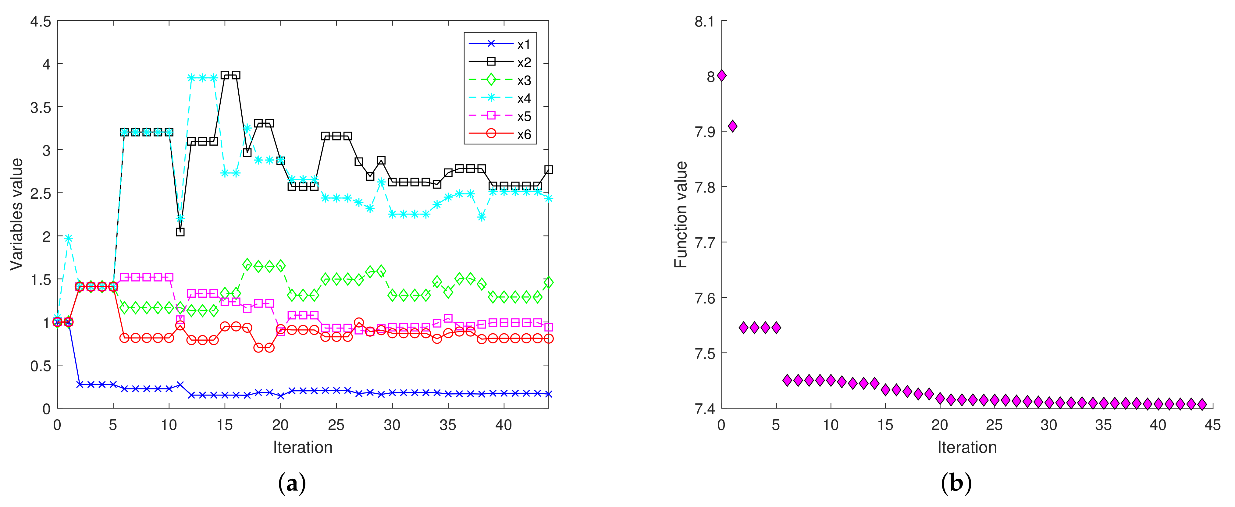
$CR=0.0504$. Hence, the reconstructed matrix $\mathbf{A}$ is acceptable, referring to Saaty’s 0.1 cut-off rule. In addition, the first 44 iterations and values of the variables for each iteration are provided in Table 3 and in Figure 2, respectively. The first graph in Figure 2 shows the evolution of the variables with respect to the number of iterations. Moreover, the convergence of the variables is not monotone. This is mainly due to the contraction step. For example, when we look at the value of $x_2$ at iterations 11, 18, and 27, it fluctuates. Furthermore, the value of ${\lambda }_{max}$ in Table 3 at iterations 2 and 6 drops significantly due to the expansion step.

Table 3. Iteration number, incumbent optimal value of ${\lambda }_{max}$, and simplex procedure for minimization (13).

Iter	Min ${\mathit{\lambda }}_{\mathit{max}}$	Procedure	Iter	Min ${\mathit{\lambda }}_{\mathit{max}}$	Procedure
0	8.00047	-	23	7.41505	contract inside
1	7.90912	initial simplex	24	7.4145	reflect
2	7.54525	expand	25	7.4145	contract inside
3	7.54525	reflect	26	7.4145	reflect
4	7.54525	reflect	27	7.4129	contract outside
5	7.54525	reflect	28	7.41214	contract outside
6	7.45024	expand	29	7.4112	contract inside
7	7.45024	reflect	30	7.40973	reflect
8	7.45024	reflect	31	7.40973	contract inside
9	7.45024	reflect	32	7.40973	contract inside
10	7.45024	reflect	33	7.40973	contract outside
11	7.44758	contract inside	34	7.40898	reflect
12	7.44479	contract outside	35	7.40884	reflect
13	7.44479	reflect	36	7.40875	contract inside
14	7.44479	reflect	37	7.40875	reflect
15	7.43308	contract inside	38	7.40868	reflect
16	7.43308	reflect	39	7.4075	reflect
17	7.43011	contract inside	40	7.4075	reflect
18	7.42561	contract inside	41	7.4075	contract outside
19	7.42561	contract inside	42	7.4075	reflect
20	7.41755	reflect	43	7.4075	reflect
21	7.41505	contract inside	44	7.40673	reflect
22	7.41505	reflect

Figure 2. The values of $x_1,\dots ,x_6$, and the first 44 iterations of the algorithm with the function value for minimization (13): (a) evolution of the variables with respect to iterations; and (b) function value vs. iteration.

In this example, we used the values for termination: $\mathtt{TolX}={10}^{-4}$, $\mathtt{TolFun}={10}^{-4}$, $\mathtt{MaxIter}=44$ and $\mathtt{MaxFunEvals}=77$. There is no significant difference in the ${\lambda }_{max}$ values after the 44th iteration.

Using the method of cyclic coordinates in [15], the optimal solution to problem (13) is ${\mathbf{x}}^{*}=(0.1618,2.7206,1.3464,2.5804,0.8960,0.7731)$. Similarly, using the least square method (LSM) in [20], the solution is ${\mathbf{x}}^{*}=(0.1651,2.7098,1.3498,2.5638,0.9103,0.7851)$. Both approaches provide the same $CR$ value in this problem, i.e., $CR=0.0504$.

5. Numerical Simulations

In this section, we validate the performance of the proposed algorithm by numerical simulations because of the following reasons. If the optimization problem is strictly convex, then the global convergence is guaranteed for one dimension (1 missing comparison). For dimension two, it may converge to a non-stationary point, though the problem is strictly convex [50]. McKinnon constructed a family of functions of two variables that are strictly convex with up to three-times continuously differentiable for which the algorithm converges to a non-stationary point. Furthermore, another version of the algorithm (adaptive Nelder-Mead algorithm, [48]) among several variants of the Nelder-Mead algorithm (see for instance, [60,61]), has been studied for high dimensional problems, but its global convergence is not well examined.

In general, the convergence properties of the proposed algorithm lack a precise statement. However, the numerical simulations could help clarify the performance of the algorithm with respect to the positive interval constraints [37]. The simulation results can provide information on how well the proposed algorithm fills an incomplete matrix, and validate its performance by considering the number of missing comparisons at large.

In the introduction, we specified that only incomplete PCMs corresponding to connected graphs are taken into account. In fact, it is also worth noting that, if the undirected graph associated with the incomplete matrix is connected, then the parameterized eigenvalue function becomes strictly convex, and therefore the optimal solution will be unique [15]. We stress again that we only consider the case of connected undirected graphs for examining the results of our simulation.

Here, it should be recalled that the Nelder-Mead algorithm directly provides the values to the missing entries. Finally, the values fill in the gap and then give the reconstructed (complete) PCMs. The simulation results obtained by the algorithm are measured by Saaty’s inconsistency ratio (CR).

5.1. Simulation Strategy

To examine the performance of the algorithm at different levels of inconsistencies, we chose two types of random PCMs:

(i)

Random matrices from the Saaty scale $\{1/9,1/8,\dots ,1/2,1,2,\dots ,8,9\}$; and

(ii)

Random consistent matrices on $[1/9,9]$ with a slight modification by multiplicative perturbation using the log-normal distribution ($\mu =0,\sigma =0.65$) which leads to inconsistent PCMs with more realistic CR values close to Saaty’s threshold $0.1$. To be more precise, the consistent matrix is modified by multiplicative perturbation U (Hadamard component-wise multiplication by U respecting the interval $[1/9,9]$ and then reconstruct the lower triangular matrix through reciprocity), where U is an upper triangular matrix generated from the log-normal distribution [62] (pp. 131–134).

Note that type (ii) matrices correspond to more reasonable real-life cases with respect to the very general type (i) matrices.

In order to construct an incomplete PCM, the procedure of an ’eliminating strategy’ in both classes of matrices with matrix size $n=4,5,6,7,8,9,10$ is given as follows. First, a complete pairwise comparison matrix is generated. Then, we remove one or more entries at random using a uniform distribution in the upper triangular first to produce a various number of missing entries for each matrix size accordingly. Subsequently, we reconstruct the lower triangle starting from the upper one to have the reciprocals of the unknowns. Furthermore, an incomplete PCM will hence be constructed. In all this, there is a test to check whether the graph is connected.

In the end, a complete PCM is reconstructed on the basis of a connected graph by applying the proposed algorithm with bound constraints on $[1/9,9]$. Furthermore, then the average CR on the 10,000 simulations will be calculated for a fixed number of missing entries (k) from the given matrix size n (a similar procedure was applied by [63] (pp. 7–8)). More precisely, the steps for calculating the average CR of the reconstructed matrices on the basis of connected graphs for both matrix types a and b are as follows:

• Fix k and n;
• Generate a random complete PCM on $[1/9,9]$;
• Make the matrix incomplete at random positions using a uniform distribution;
• Identify whether the graph associated with an incomplete matrix is connected or disconnected. If it is connected, then we apply the proposed algorithm for the optimal completion of the incomplete PCM using the same interval constraint $[1/9,9]$;
• Compute and save the CR value for the reconstructed matrix;
• Repeat steps b–e until 10,000 CR values are obtained;
• Calculate the average CR.

5.2. Simulation Results

The results of simulations of the matrix type a are reported in Table 4 and in Figure 3. The numbers reported in boldface font are calculated from the spanning trees. This happens when $k=n(n-1)/2-(n-1)=(n-1)(n-2)/2$. Such numbers do not appear in Table 4 if $n\ge 7$. Due to excessive processing time, we did not compute the average $CR$ for all $k>12$ except for some random large k values shown in Tables 6 and in 7.

Table 4. Average CR of 10,000 random matrices from the Saaty scale.

	Matrix Size n
$\mathit{k}$	4	5	6	7	8	9	10
0	1.0028	1.0007	1.0022	0.9990	0.9988	1.0003	1.0008
1	0.6512	0.8350	0.9022	0.9357	0.9556	0.9675	0.9728
2	0.3432	0.6682	0.8091	0.8731	0.9117	0.9365	0.9497
3	0.0602	0.4983	0.7094	0.8066	0.8651	0.8989	0.9217
4	−	0.3460	0.6062	0.7479	0.8219	0.8667	0.8940
5	−	0.1904	0.5107	0.6744	0.7688	0.8338	0.8695
6	−	0.0530	0.4113	0.6094	0.7296	0.8012	0.8447
7	−	−	0.3161	0.5429	0.6768	0.7631	0.8209
8	−	−	0.2168	0.4773	0.6348	0.7292	0.7907
9	−	−	0.1313	0.4125	0.5855	0.6979	0.7647
10	−	−	0.0481	0.3445	0.5420	0.6612	0.7369
11	−	−	−	0.2811	0.4944	0.6278	0.7128
12	−	−	−	0.2144	0.4432	0.5914	0.6845

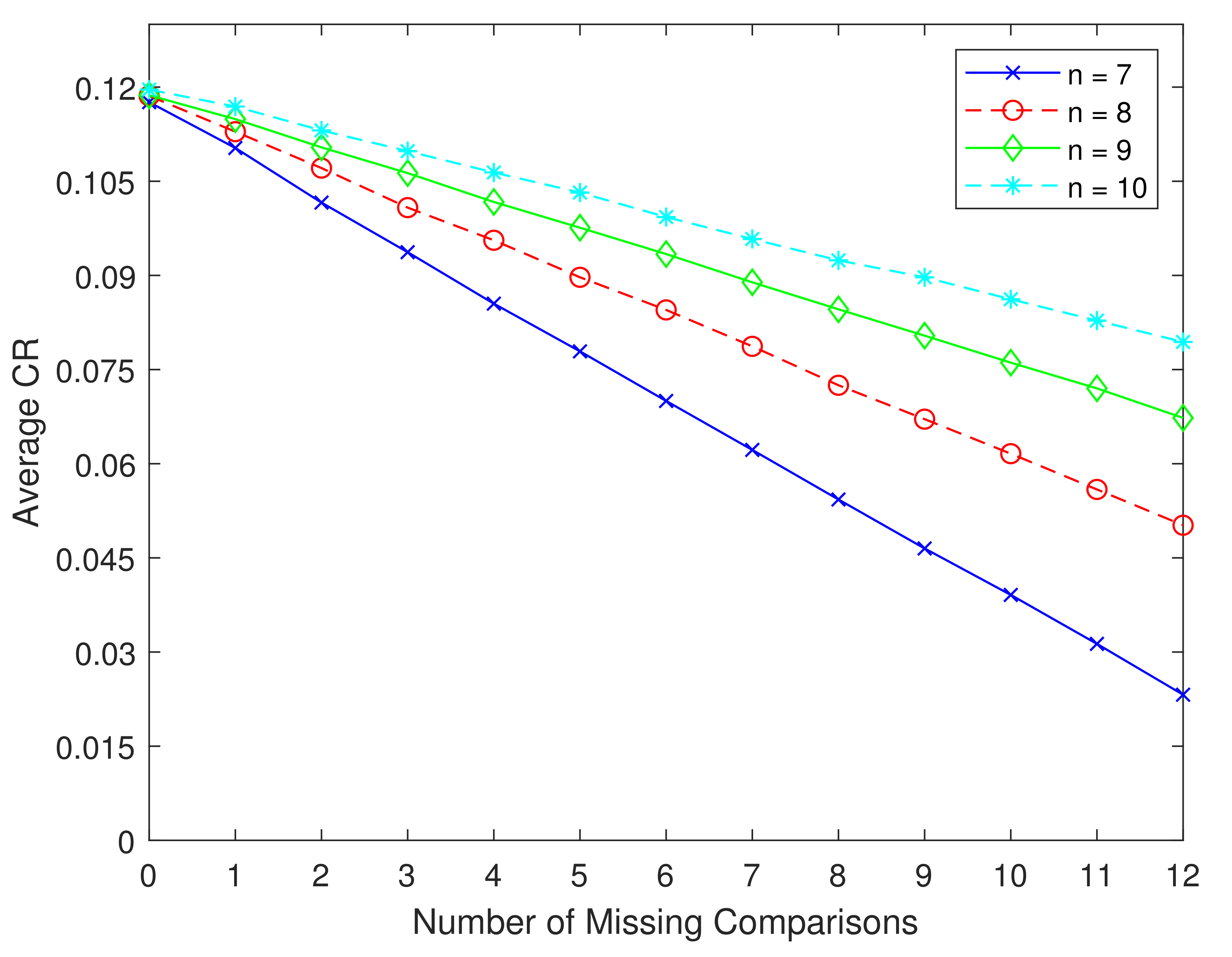
Figure 3. Average $CR$ of 10,000 matrices vs. the number of missing comparisons k with respect to the matrix size n corresponding to Table 4.

The first row in Table 4 represents the average CR of the original matrices when the number of missing entries is null, i.e., $k=0$. It can be observed that the average CR decreases across the columns when the number of missing entries rises in each matrix size n. On the contrary, the sequence is increasing across all rows with the exception of $k=0$. Note that our ’initial complete matrices are, on average, inconsistent.

The relations between the number of missing comparisons (k) and their respective average CR are depicted in Figure 3. As it can be seen from all line graphs, they are decreasing for each n while the number of missing comparisons (k) is increasing.

Having the same type of simulations work, the average values of CR obtained from the matrix type b are presented in Table 5 and in Figure 4. The numbers that appear in boldface font are also calculated from the spanning trees. The results are similar to Table 4 and Figure 3 in terms of monotonic values. An interesting simulation result, in this case, is that the average CR values of the last row in each column are less than Saaty’s threshold 0.1, even though the initial complete matrices had a $CR$, on average, greater than 0.1.

Table 5. Average $CR$ of 10,000 modified consistent matrices using log-normal distribution.

	Matrix Size n
$\mathit{k}$	4	5	6	7	8	9	10
0	0.1210	0.1178	0.1171	0.1176	0.1186	0.1187	0.1196
1	0.0802	0.0974	0.1050	0.1103	0.1129	0.1149	0.1169
2	0.0405	0.0787	0.0938	0.1016	0.1071	0.1104	0.1131
3	$\mathbf{0.0020}$	0.0578	0.0809	0.0937	0.1008	0.1063	0.1098
4	−	0.0373	0.0700	0.0855	0.0956	0.1017	0.1064
5	−	0.0211	0.0576	0.0779	0.0897	0.0976	0.1032
6	−	$\mathbf{0.0020}$	0.0462	0.0700	0.0845	0.0934	0.0993
7	−	−	0.0345	0.0622	0.0787	0.0889	0.0958
8	−	−	0.0234	0.0543	0.0725	0.0846	0.0924
9	−	−	0.0125	0.0465	0.0671	0.0804	0.0897
10	−	−	$\mathbf{0.0019}$	0.0391	0.0616	0.0761	0.0862
11	−	−	−	0.0313	0.0559	0.0720	0.0828
12	−	−	−	0.0232	0.0502	0.0673	0.0794

Figure 4. Average $CR$ of 10,000 matrices vs. number of missing comparisons k with respect to the matrix size n corresponding to Table 5.

In our simulations, we observed the performance of the algorithm by taking the matrix size n from 4 up to 10, and the number of missing comparisons (k) up to 12 because of excessive computational time. However, the average CR for some number of missing comparisons (k) are reported in Table 6 and Table 7, in order to examine the efficiency of the algorithm for large k. Since our simulation results are based on connected graphs, the eigenvalue function is strictly convex and therefore the optimal solutions obtained by the proposed algorithm are unique. Moreover, the algorithm provides more consistent PCMs with more incomplete information. This means that when k is closer to $n(n-1)/2$.

Table 6. Average CR of 10,000 random matrices from the Saaty scale for an arbitrarily large number of missing comparisons k with respect to matrix size n that continued from Table 4.

	$\mathit{n}=8$		$\mathit{n}=9$		$\mathit{n}=10$
$\mathit{k}$	Average CR	$\mathit{k}$	Average CR	$\mathit{k}$	Average CR	$\mathit{k}$	Average CR
13	0.3935	14	0.5186	20	0.4634	31	0.1553
15	0.3011	16	0.4479	25	0.3236	32	0.1308
18	0.1621	17	0.4112	28	0.2361	33	0.1032
19	0.1206	22	0.2312	29	0.2091	35	0.0568
21	0.0436	23	0.1953	30	0.1819	36	0.0350

Table 7. Average CR of 10,000 modified consistent matrices for an arbitrarily large number of missing comparisons k with respect to matrix size n that continued from Table 5.

	$\mathit{n}=8$		$\mathit{n}=9$		$\mathit{n}=10$
$\mathit{k}$	Average CR	$\mathit{k}$	Average CR	$\mathit{k}$	Average CR	$\mathit{k}$	Average CR
13	0.0444	14	0.0592	20	0.0523	31	0.0169
15	0.0335	16	0.0506	25	0.0364	33	0.0136
18	0.0171	17	0.0461	28	0.0263	33	0.0106
19	0.0125	22	0.0252	29	0.0232	35	0.0049
21	0.0024	23	0.0212	30	0.0199	36	0.0021

We conclude that the algorithm performs well and is capable of providing an optimal completion for the incomplete PCM up to $k=(n-1)(n-2)/2$. Furthermore, due to the connectedness of the associated undirected graphs used in our numerical simulations, the optimal solutions obtained by the method are unique (from Theorem 1).

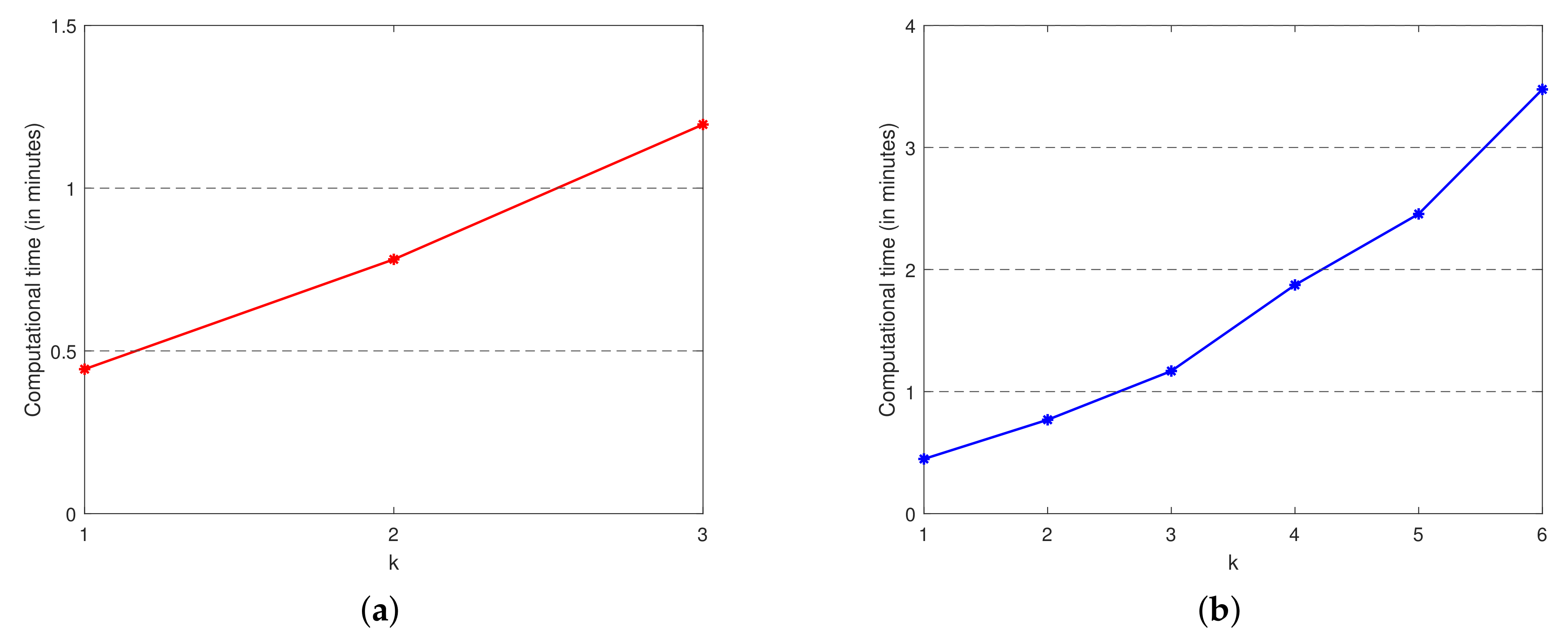
The computation time of the proposed algorithm to reconstruct complete PCMs from the incomplete PCMs and then to calculate the average CR of 10,000 completed PCMs versus to the number of missing comparisons k corresponding to Table 4 for matrices of size $n=4,5,6,7,8,9,10$ is shown in Figure 5. The computation time is calculated using MATLAB’s tic-toc function. As can be seen in Figure 5, at each matrix size n, the computation time increases when the number of missing comparisons (k) increases. Note that the execution time excludes the formation of the initial and incomplete matrices in the process.

Figure 5. Computational time for the average $CR$ of 10,000 matrices vs. number of missing comparisons k with respect to matrix size n corresponding to Table 4: (a) $n=4$; (b) $n=5$; (c) $n=6$; and (d) $n=7,8,9,10$.

All simulation results were run on a laptop (Intel(R) core(TM) i5-8250u, CPU: 1.80 GHz and RAM: 16 GB) using MATLAB (R2020b).

6. Conclusions

In this paper, we studied an application of the Nelder-Mead algorithm to the constrained `${\lambda }_{max}$-optimal completion’ and provided numerical simulations to study its performance. Our simulation results indicate that the proposed algorithm is capable of estimating the missing values in the incomplete PCMs, and it is simple, adaptable and efficient. Furthermore, the obtained solution is unique if and only if the undirected graph underlying the incomplete PCM is connected (by Theorem 1). It should be noted that the associated graph is necessarily connected if $k\le n-2$ and possibly connected if there are at most $k=(n-1)(n-2)/2$ missing comparisons. If $k>(n-1)(n-2)/2$, the graph is not connected because the number of known entries in the incomplete matrix is less than $n-1$ (see, e.g., [63] (p. 7)). Most importantly, the average CR in Table 4 and Table 5 are calculated on the basis of connected undirected graphs.

Our proposal has its roots in the most widely used inconsistency index, as the $CR$ proposed by Saaty. If, on the one hand, the $CR$ was considered the standard for the quantification of inconsistency, on the other hand, its role has been limited to this simple task. Its use for other purposes, as for instance, the optimal completion of pairwise comparisons matrices, has been impaired by its perception as a function difficult to treat. One of the purposes of this paper is also to help demystify this view.

The future research could be a comparative analysis of the algorithm with other optimal completion methods (see for instance, refs. [13,15,18,20,64]).

References

- Hammond, J.S.; Keeney, R.L.; Raiffa, H. Smart Choices: A Practical Guide to Making Better Decisions; Harvard Business School Press: Boston, MA, USA, 1999. [Google Scholar]
- Saaty, T.L. A scaling method for priorities in hierarchical structures. J. Math. Psychol. 1977, 15, 234–281. [Google Scholar] [CrossRef]
- Saaty, T.L. The Analytic Hierarchy Process; McGraw-Hill: New York, NY, USA, 1980. [Google Scholar]
- Keeney, R.; Raiffa, H.; Rajala, D.W. Decisions with Multiple Objectives: Preferences and Value Trade-Offs. IEEE Trans. Syst. Man Cybern. 1979, 9, 403. [Google Scholar] [CrossRef]
- Rezaei, J. Best-worst multi-criteria decision-making method. Omega 1977, 53, 49–57. [Google Scholar] [CrossRef]
- Figueira, J.R.; Mousseau, V.; Roy, B. ELECTRE methods. Multiple Criteria Decis. Anal. 2016, 155–185. [Google Scholar]
- Qi, X.; Yu, X.; Wang, L.; Liao, X.; Zhang, S. PROMETHEE for prioritized criteria. Soft Comput. 2019, 23, 11419–11432. [Google Scholar] [CrossRef]
- Bana e Costa, C.A.; De Corte, J.-M.; Figueira, J.R.; Vansnick, J.C. On the Mathematical Foundations of MACBETH in Multiple Criteria Decision Analysis: State of the Art Surveys; Figueira, J., Greco, S., Ehrgott, M., Eds.; The London School of Economics and Political Science: London, UK, 2005. [Google Scholar]
- Hansen, P.; Ombler, F. A new method for scoring additive multi-attribute value models using pairwise rankings of alternatives. J. Multiple Criteria Decis. Anal. 2008, 15, 87–107. [Google Scholar] [CrossRef]
- Lin, C.-C. A revised framework for deriving preference values from pairwise comparison matrices. Eur. J. Oper. Res. 2007, 176, 1145–1150. [Google Scholar] [CrossRef]
- Harker, P.T. Incomplete pairwise comparisons in the Analytic Hierarchy Process. Math. Model. 1987, 9, 837–8487. [Google Scholar] [CrossRef]
- Shiraishi, S.; Obata, T. On a maximization problem arising from a positive reciprocal matrix in AHP. Bull. Inform. Cybern. 2002, 34, 91–96. [Google Scholar] [CrossRef]
- Shiraishi, S.; Obata, T. Properties of a positive reciprocal matrix and their application to AHP. J. Oper. Res. Soc. Jpn. 1998, 41, 404–414. [Google Scholar] [CrossRef]
- Ábele-Nagy, K. Minimization of the Perron eigenvalue of incomplete pairwise comparison matrices by Newton iteration. Acta Univ. Sapientiae Inform. 2015, 7, 58–71. [Google Scholar] [CrossRef]
- Bozóki, S.; Fülöp, J.; Rónyai, L. On optimal completion of incomplete pairwise comparison matrices. Math. Comput. Model. 2010, 52, 318–333. [Google Scholar] [CrossRef]
- Tekile, H.A. Gradient Descent Method for Perron Eigenvalue Minimization of Incomplete Pairwise Comparison Matrices. Int. J. Math. Appl. 2019, 7, 137–148. [Google Scholar]
- Brunelli, M. A survey of inconsistency indices for pairwise comparisons. Int. J. Gen. Syst. 2015, 47, 751–771. [Google Scholar] [CrossRef]
- Fedrizzi, M.; Giove, S. Incomplete pairwise comparison and consistency optimization. Eur. J. Oper. Res. 2007, 183, 303–313. [Google Scholar] [CrossRef]
- Benítez, J.; Delgado-Galván, X.; Izquierdo, J.; Pérez-García, R. Consistent completion of incomplete judgments in decision making using AHP. J. Comput. Appl. Math. 2015, 290, 412–422. [Google Scholar] [CrossRef]
- Ergu, D.; Kou, G.; Peng, Y.; Zhang, M. Estimating the missing values for the incomplete decision matrix and consistency optimization in emergency management. Appl. Math. Model. 2016, 40, 254–267. [Google Scholar] [CrossRef]
- Zhou, X.; Hu, Y.; Deng, Y.; Chan, F.T.S.; Ishizaka, A. A DEMATEL-based completion method for incomplete pairwise comparison matrix in AHP. Ann. Oper. Res. 2018, 271, 1045–1066. [Google Scholar] [CrossRef]
- Kułakowski, K. On the geometric mean method for incomplete pairwise comparisons. Mathematics 2020, 8, 1873. [Google Scholar] [CrossRef]
- Alrasheedi, M. Incomplete pairwise comparative judgments: Recent developments and a proposed method. Decis. Sci. Lett. 2019, 8, 261–274. [Google Scholar] [CrossRef]
- Brunelli, M.; Fedrizzi, M.; Giove, S. Reconstruction methods for incomplete fuzzy preference relations: A numerical comparison. Int. Workshop Fuzzy Log. Appl. 2007, 86–93. [Google Scholar]
- Harker, P.T. Alternative modes of questioning in the Analytic Hierarchy process. Math. Model. 1987, 9, 353–360. [Google Scholar] [CrossRef]
- Ureña, R.; Chiclana, F.; Morente-Molinera, J.A.; Herrera-Viedma, E. Managing incomplete preference relations in decision making: A review and future trends. Inf. Sci. 2015, 302, 14–32. [Google Scholar] [CrossRef]
- Arbel, A.; Vargas, L.G. Preference simulation and preference programming: Robustness issues in priority derivation. Eur. J. Oper. Res. 1993, 69, 200–209. [Google Scholar] [CrossRef]
- Saaty, T.L.; Vargas, L.G. Uncertainty and rank order in the Analytic Hierarchy Process. Eur. J. Oper. Res. 1987, 32, 107–117. [Google Scholar] [CrossRef]
- Salo, A.; Hämäläinen, R.P. Preference assessment by imprecise ratio statements. Oper. Res. 1992, 40, 1053–1061. [Google Scholar] [CrossRef]
- Wang, Z.-J. Eigenvector driven interval priority derivation and acceptability checking for interval multiplicative pairwise comparison matrices. Comput. Ind. Eng. 2021, 156, 107–215. [Google Scholar] [CrossRef]
- Obata, T.; Shunsuke, S. Computational study of characteristic polynomial of 4th order PCM in AHP. Bull. Inform. Cybern. 2021, 1–12. [Google Scholar] [CrossRef]
- Alonso, J.A.; Lamata, M.T. Consistency in the Analytic Hierarchy Process: A new approach. Int. J. Uncertain. Fuzziness Knowl. Based Syst. 2006, 14, 445–459. [Google Scholar] [CrossRef]
- Nelder, J.A.; Mead, R. A simplex method for function minimization. Comput. J. 1965, 7, 308–313. [Google Scholar] [CrossRef]
- D’Errico, J. Fminsearchbnd, Fminsearchcon File Exchange—MATLAB Central. Available online: https://it.mathworks.com/matlabcentral/fileexchange/8277-fminsearchbnd-fminsearchcon (accessed on 16 February 2021).
- Mehta, V.K.; Dasgupta, B. A constrained optimization algorithm based on the simplex search method. Eng. Optim. 2012, 44, 537–550. [Google Scholar] [CrossRef]
- Oldenhuis, R. Optimize. MathWorks File Exchange. Available online: https://it.mathworks.com/matlabcentral/fileexchange/24298-minimize (accessed on 16 May 2021).
- Gill, P.E.; Murray, W.; Wright, M.H. Practical Optimization; SIAM: Philadelphia, PA, USA, 2019. [Google Scholar]
- Tepljakov, A. Fractional-Order Modeling and Control of Dynamic Systems; Springer: Berlin, Germany, 2017. [Google Scholar]
- Lagarias, J.C.; Reeds, J.A.; Wright, M.H.; Wright, P.E. Convergence properties of the Nelder-Mead simplex method in low dimensions. SIAM J. Optim. 1998, 9, 112–147. [Google Scholar] [CrossRef]
- Nocedal, J.; Wright, S. Numerical Optimization, 2nd ed.; Springer Science & Business Media: Berlin/Heidelberg, Germany, 2006; pp. 238–240. [Google Scholar]
- Singer, S.; Nelder, J. Nelder-Mead algorithm. Scholarpedia 2009, 4, 2928. [Google Scholar] [CrossRef]
- Wright, M. Direct search methods: Once scorned, now respectable. In Numerical Analysis: Proceedings of the 1995 Dundee Biennial Conference in Numerical Analysis; Addison-Wesley: Boston, MA, USA, 1996; pp. 191–208. [Google Scholar]
- Press, W.H.; Teukolsky, S.A.; Vetterling, W.T.; Flannery, B.P. Numerical Recipes in C: The Art of Scientific Computing, 2nd ed.; University of Cambridge: Cambridge, UK, 1992. [Google Scholar]
- The MathWorks, Inc. MATLAB’s Fminsearch Documentation. Available online: https://it.mathworks.com/help/optim/ug/fminsearch-algorithm.html (accessed on 16 May 2021).
- Kochenderfer, M.J.; Wheeler, T.A. Algorithms for Optimization; MIT Press: London, UK, 2019; pp. 105–108. [Google Scholar]
- Weisstein, E.W. “Nelder-Mead Method.” From MathWorld—A Wolfram Web Resource. Available online: https://mathworld.wolfram.com/Nelder-MeadMethod.html (accessed on 16 July 2021).
- Kelley, C.T. Detection and remediation of stagnation in the Nelder-Mead algorithm using a sufficient decrease condition. SIAM J. Optim. 1999, 10, 43–55. [Google Scholar] [CrossRef]
- Gao, F.; Han, L. Implementing the Nelder-Mead simplex algorithm with adaptive parameters. Comput. Optim. Appl. 2012, 51, 259–277. [Google Scholar] [CrossRef]
- Lagarias, J.C.; Poonen, B.; Wright, M.H. Convergence of the Restricted Nelder-Mead Algorithm in Two Dimensions. SIAM J. Optim. 2012, 22, 501–532. [Google Scholar] [CrossRef]
- McKinnon, K.I. Convergence of the Nelder-Mead Simplex method to a nonstationary Point. SIAM J. Optim. 1998, 176, 148–158. [Google Scholar] [CrossRef]
- Singer, S.; Singer, S. Complexity analysis of Nelder-Mead search iterations. In Proceedings of the 1. Conference on Applied Mathematics and Computation; PMF–Matematicki Odjel: Zagreb, Croatia, 1999; pp. 185–196. [Google Scholar]
- Singer, S.; Singer, S. Efficient implementation of the Nelder-Mead search algorithm. Appl. Numer. Anal. Comput. Math. 2004, 1, 524–534. [Google Scholar] [CrossRef]
- Takahama, T.; Sakai, S. Constrained optimization by applying the α constrained method to the nonlinear simplex method with mutations. IEEE Trans. Evol. Comput. 2005, 9, 437–451. [Google Scholar] [CrossRef]
- Deb, K.; Agrawal, S.; Pratap, A.; Meyarivan, T. A fast elitist non-dominated sorting genetic algorithm for multi-objective optimization: NSGA-II. In Proceedings of the International Conference on Parallel Problem Solving from Nature, Leiden, The Netherlands, 5–9 September 2000; pp. 849–858. [Google Scholar]
- Pham, D.; Ghanbarzadeh, A.; Koc, E.; Otri, S.; Rahim, S.; Zaidi, M. The Bees Algorithm; Technical Note; Manufacturing Engineering Centre, Cardiff University: Cardiff, UK, 2005. [Google Scholar]
- Baudin, M.; Nelder-Mead User’s Manual. Consortium Scilab-Digiteo. 2010. Available online: http://forge.scilab.org/upload/docneldermead/files/neldermead.pdf (accessed on 15 October 2020).
- Kelley, C.T. Iterative Methods for Optimization; SIAM: Philadelphia, PA, USA, 1999. [Google Scholar]
- Shiraishi, S.; Tsuneshi, O. Some remarks on the maximum eigenvalue of 3rd order pairwise comparison matrices in AHP. Obata Bull. Inform. Cybern. 2021, 53, 1–13. [Google Scholar] [CrossRef]
- Benítez, J.; Delgado-Galván, X.; Izquierdo, J.; Pérez-García, R. Achieving matrix consistency in AHP through linearization. Appl. Math. Model. 2011, 35, 4449–4457. [Google Scholar] [CrossRef]
- Byatt, D. Convergent Variants of the Nelder-Mead Algorithm. Master’s Thesis, University of Canterbury, Canterbury, UK, 2000. [Google Scholar]
- Price, C.J.; Coope, I.D.; Byatt, D. A convergent variant of the Nelder-Mead algorithm. J. Optim. Theory Appl. 2002, 113, 5–19. [Google Scholar] [CrossRef]
- Forbes, C.; Evans, M.; Hastings, N.; Peacock, B. Statistical Distributions, 4th ed.; John Wiley & Sons, Inc.: Hoboken, NJ, USA, 2011; pp. 131–134. [Google Scholar]
- Ágoston, K.C.; Csató, L. Extension of Saaty’s inconsistency index to incomplete comparisons: Approximated thresholds. arXiv 2021, arXiv:2102.10558. [Google Scholar]
- Koczkodaj, W.W.; Herman, M.W.; Orlowski, M. Managing null entries in pairwise comparisons. Knowl. Inf. Syst. 1999, 1, 119–125. [Google Scholar] [CrossRef][Green Version]
Publisher’s Note: MDPI stays neutral with regard to jurisdictional claims in published maps and institutional affiliations. |
© 2021 by the authors. Licensee MDPI, Basel, Switzerland. This article is an open access article distributed under the terms and conditions of the Creative Commons Attribution (CC BY) license (https://creativecommons.org/licenses/by/4.0/).