Multi-Objective Task Scheduling Optimization in Spatial Crowdsourcing

Abstract

Recently, with the development of mobile devices and the crowdsourcing platform, spatial crowdsourcing (SC) has become more widespread. In SC, workers need to physically travel to complete spatial–temporal tasks during a certain period of time. The main problem in SC platforms is scheduling a set of proper workers to achieve a set of spatial tasks based on different objectives. In actuality, real-world applications of SC need to optimize multiple objectives together, and these objectives may sometimes conflict with one another. Furthermore, there is a lack of research dealing with the multi-objective optimization (MOO) problem within an SC environment. Thus, in this work we focused on task scheduling based on multi-objective optimization (TS-MOO) in SC, which is based on maximizing the number of completed tasks, minimizing the total travel costs, and ensuring the balance of the workload between workers. To solve the previous problem, we developed a new method, i.e., the multi-objective task scheduling optimization (MOTSO) model that consists of two algorithms, namely, the multi-objective particle swarm optimization (MOPSO) algorithm with our fitness function Alabbadi, et al. and the ranking strategy algorithm based on the task entropy concept and task execution duration. The main purpose of our ranking strategy is to improve and enhance the performance of our MOPSO. The primary goal of the proposed MOTSO model is to find an optimal solution based on the multiple objectives that conflict with one another. We conducted our experiment with both synthetic and real datasets; the experimental results and statistical analysis showed that our proposed model is effective in terms of maximizing the number of completed tasks, minimizing the total travel costs, and balancing the workload between workers.

1. Introduction

Crowdsourcing is an outsourcing platform that facilitates the achievement of time-consuming and costly tasks. It is an optimal way to solve complicated problems that need human intelligence [1]. Spatial crowdsourcing (SC) is a kind of crowdsourcing that is referred to as geo-crowdsourcing or location-aware crowdsourcing. In SC, workers must travel physically to a specific location to complete spatial–temporal tasks, such as taking pictures and videos, gathering weather information, computing the noise level, and observing waiting times of restaurant and food delivery. In fact, SC is popular in the research community and industry.

SC consists of multiple agents that interact with one another: the requester who publishes tasks on the platform, the worker who moves to locations in order to complete the requested tasks, and the SC server who connects the requester and the worker. SC also has primary challenges, i.e., task assignment, incentive mechanism, security and privacy threats, and quality control. Most of the critical issues depend on task assignment, and so the task assignment issue is a core challenge of SC [2,3,4], which refers to assigning particular tasks to suitable workers who should finish these tasks under specific goals and time constraints.

SC can be classified based on three aspects according to [5,6], as presented in Figure 1. The first classification is the worker’s motivation, which can be classified into two types: reward-based and voluntary. Reward-based workers should complete SC tasks correctly to receive a particular reward, while voluntary workers are self-incentivized to complete a spatial task. The second aspect in the SC classification is the task publishing mode, which is classified into the server-assigned task (SAT) mode, where the server assigns available tasks to suitable workers according to the optimal goal, and the worker-selected task (WST) mode, where the workers select any task based on the optimal goal. The third SC classification is based on the numbers of workers, meaning that tasks can be assigned to a single reliable worker or to multiple workers, if most of the workers are reliable. Indeed, in the SAT mode, the server has full control to assign a task to a suitable worker. Therefore, the server can design more optimization techniques to increase the throughput of the system and to provide a balanced workload for each worker [7]. Based on this, in this work, we relied on the SAT mode to design an effective model commensurate with our objectives. The shaded rectangles in Figure 1 indicate the categories we focused on in this work.

Figure 1. A classification of spatial crowdsourcing. Reward = reward-based worker; voluntary = voluntary-based worker; SAT = server-assigned task; WST = worker-selected task; single = single worker; multiple = multiple workers.

In SC, the task assignment issue has been formulated as task matching [4,6,8,9] or task scheduling [2,10,11]. Regarding continuous movement between locations in SC, each worker must adopt an optimal plan in order to complete each task assigned to him/her according to certain predefined objectives. Therefore, the task assignment problem needs to direct its attention to the task scheduling problem [5]. In contrast, real applications of SC need to optimize several objectives at the same time in order to benefit from SC, some of which may conflict with one another [5]. However, very few studies have addressed the problem of multi-objective optimization (MOO) within an SC environment; therefore, MOO must be considered in SC. Thus, we formulated a novel solution for the problem in SC, namely, task scheduling based on multi-objective optimization (TS-MOO) in SC. We focused on optimizing three primary conflicting objectives that have the same importance, i.e., maximizing the number of completed tasks (|V|), minimizing the total travel costs (TTCs), and ensuring a balance of the workload between workers (WLB). The workload balance between workers is essential in SC, as it helps to avoid overload between workers but this objective is often ignored [5]; additionally, reaching a balanced workload between workers is useful for speeding up the completion of requested tasks [2,12].

Meta-heuristic algorithms, such as particle swarm optimization (PSO), have been used to resolve task scheduling problems [13,14,15]. PSO was first discovered by Eberhart [16], who was inspired by the social behavior of animals. PSO has many advantages [17], including the simplicity in its concepts, its durability of parameters, being easy to implement, being able to achieve the optimal solution quickly, and being fast in terms of controlling the computation. Additionally, PSO has the ability to find an optimal solution in different applications. For instance, it was extended to multi-objective particle swarm optimization (MOPSO) in order to solve MOO effectively by [18] when merging the advantages of PSO and MOO.

This research aims to find an optimal multi-objective task scheduling approach based on the three conflicting objectives mentioned previously. Thus, we propose the multi-objective task scheduling optimization (MOTSO) model, which involves two primary novel algorithms. The first algorithm is based on a relatively new fitness function, which was introduced in detail in our previous work [19], while the second algorithm is the ranking strategy algorithm, which is discussed in this paper. The main goal of the ranking strategy algorithm is to improve and enhance the performance of our MOPSO.

The motivation for this work stems from the fact that in recent years, many governments have become interested in geographical or spatial tasks such as gathering geographic data and measuring spatial data within SC [5]. Moreover, geographical information has great importance to people’s daily lives [20]. Thus, there are many applications that are used for different purposes, e.g., Uber [21], which is a taxi ride-sharing application; Google Maps [22] and Waze [23], which are GPS-based geographical navigation applications that allow drivers to share traffic and road information in a quick and easy manner; and Yelp [24], which is a food discovery and delivery service. Other successful examples include TaskRabbit [25], which provides household tasks and home services, and Gigwalk [26], which is a marketplace for sensing tasks such as geo-images, videos, or collecting answers about stores. These are only some examples of the available applications, as there are many other applications with a range of purposes.

Despite the attention paid to the SC field, most of the previous research in this area did not address the TS-MOO problem, which deals with the three conflicting objectives in SC. Our motivation is based on the fact that there is a need for a method that addresses the TS-MOO problem in SC, in order to determine the optimal scheduling for a task based on the three primary conflicting objectives mentioned, which are adopted in this study and treated with equal importance.

An additional example is the accident reporting application to manage accident-related activities; in more detail, when a traffic accident occurs and there are no casualties, one party (the requester) will send a request to the platform. The platform (server) will then assign this task to a suitable worker; the worker must attend the location of the accident to investigate and will receive the details related to the accident in order to determine the responsibility between all parties involved. Then, the worker will issue an accident report that contains all of the details (such as a photograph of the accident and damage evaluation reports) to all parties involved in the incident. This platform aims to assist the traffic police in order to enhance road safety and to provide better monitoring for field operations. Figure 2 shows a certain scenario that we have set up for SC.

Figure 2. A spatial crowdsourcing (SC) scenario of the multi-objective task scheduling optimization (MOTSO) model.

In Figure 2, $t_{j }= ⟨l_{t_j},d_{t_j}⟩$ $l_{t_j}$ is the location of the task, and $d_{t_j}$ is the time duration of a task. Meanwhile, the two sets for the server are tasks $T= \left\{t_1, t_2, t_3, \dots t_n\right\}$ and workers W= {$w_1, w_2, w_3, \dots w_{m }\}$. The requesters send a query (SC-Query), which includes the task and its constraints, to the SC server. Then, any available workers would consequently send their locations to the server. Thus, each requested task is assigned to a certain worker by the server. The workers should be assigned tasks in a manner that achieves the maximum number of completed tasks by minimizing the total traveled distance by the worker to complete said tasks. Applying this scenario to the accident reporting application mentioned previously will lead to covering a large number of accidents with minimal travel costs. At the same time, it will allow for distributing tasks between workers fairly in order to avoid the overload of the workers and to reach a balanced workload among them. Indeed, the worker must move within a certain plan and in a perfect way between the different locations to complete their assigned tasks. Therefore, the server must achieve optimal scheduling based on the three objectives mentioned earlier.

With the above in mind, we propose the MOTSO model to deal with the conflicting objectives in order to achieve optimal task scheduling; the assumptions underlying our model are that workers are volunteers, that each worker should complete one task only, and that all workers are reliable. We tested our model using real and synthetic datasets, and we conducted extensive experiments to evaluate the performance of the MOTSO model. The results of our experiments show the effectiveness of the proposed model for small- and large-scale environments.

2. Related Work

Recently, the spatial crowdsourcing field has gained much attention in both research and industry communities, e.g., Gigwalk and TaskRabbit. There are many surveys in the SC area (e.g., [5,27,28,29,30]) that mention the main taxonomy, challenges, and general techniques of task assignment in SC. A general example of SC is Gmission, which was developed by [20]. Gmission is a typical SC platform that has location-dependent tasks. This means that the system assigns spatial tasks to nearby workers. Thus, the workers should go to a particular location to complete the assigned tasks. This system allows individuals to register on the platform through the interface model to post tasks. After this, they can collect answers to their tasks, which are submitted in a specific format by the worker after executing them. The system can check whether the worker has reached the location of their assigned tasks by tracing the worker’s location upon their submitted answer.

In this section, we review the most common research works that have studied the task assignment problem in SC. The task assignment problem is formulated as either the task matching problem [3,4,6,8,9,12,31,32,33] or the task scheduling problem [2,7,10,11], depending on the objective to be achieved. In contrast, there are limited studies that have highlighted the MOO in SC. We display our related works regarding three aspects commensurate with our research aspects as follows: task matching in SC, task scheduling in SC, and the binary-objective optimization problem in SC.

2.1. Task Matching in SC

Some studies have focused on an SC task matching technique to solve diverse objectives. For instance, Kazemi et al. [6] presented a framework in the SAT mode, and they assumed all workers are reliable in SC. The main objective of [6] was to solve the maximum task assignment (MTA). The researchers formulated MTA as a matching problem, and then they tried to solve MTA by reducing the maximum flow problem. In more detail, the worker’s reliability was integrated into the framework mentioned in [6] by Kazemi et al. [9]. They tried to maximize the number of assigned tasks that require many confident workers to achieve these tasks [9]. They focused on the maximum correct task assignment (MCTA) problem and tried to solve it by proposing three approaches based on the 3D matching technique. Furthermore, other studies such as [8,31] associated each worker to a task using a skill score under different constraints. Kazemi et al. [31] extended the framework of [6] by considering the expertise score of a worker and the maximum score assignment (MSA). For instance, when online workers are ready, they send their inquiry—which includes their region, capacity, and expertise—to the SC server. Then, the SC server matches each task to one worker under satisfying constraints. This framework proposes three heuristic algorithms based on MWBM that aim to maximize the score of the assignment task. In [8], multi-skill SC (MS-SC) was considered as an approach for finding suitable workers under multi-skill task, budget, and time/distance constraints with the maximum score. Then, three approximate approaches were proposed, i.e., the greedy-based matching, greedy divide-and-conquer (g-D&C), and cost model-based adaptive algorithms.

Real-time matching is considered in SC as mentioned in [3,4,12,32]. For instance, maximizing the total utility score is the main objective of both [3,4]. The authors in [3] addressed the global online micro-task allocation problem in SC. They proposed the two-phase global online allocation algorithm (TGOA) to solve the proposed problem, by dividing a set of tasks and workers into groups based on their order of arrival order. The first group was allocated a greedy assignment to find the highest utility value between the workers and the tasks, while the second group adopted an optimal strategy to find the optimal match between the workers and the tasks. Then, the authors proposed the greedy TGOA algorithm to improve the efficiency and scalability of TGOA. Meanwhile, Song et al. [4] introduced a trichromatic online matching problem in real-time SC. They considered three sides or objects, i.e., task, worker, and workplace, during the assignment. They reduced the problem to the 3D matching problem and then solved it by introducing the greedy and threshold-based randomized algorithm to improve the performance of the greedy algorithm in terms of maximizing the utility score. This model is suitable only for SC applications that require a workplace.

Moreover, the real-time framework proposed in [32] can solve the hyper-local SC problem, where the task is assigned to the closest worker within a circular region. The main challenge in [32] was to maximize the assigned task under budget constraints. The authors investigated the problem under two variants; the first variant was a fixed budget, under which the authors proposed two heuristic algorithms. The second variant was a dynamic budget, under which they proposed two algorithms to solve the problem. Factually, the hyper-local approach discussed in [32] means the worker might not need to travel to complete a spatial task, which is not applicable to most SC applications such as home delivery services and Uber. Therefore, we did not focus on the hyper-local SC in our study.

In [33], the task assignment problem in SC was considered as a distributed environment to ensure the maximization of the number of workers and tasks arriving in a short time. The authors solved the mentioned task assignment problem in a parallel fashion using the partition method over cloud servers.

In the continual movement between locations in SC, each worker should have an optimal way to complete the assigned tasks under predefined constraints. Subsequently, it is necessary to focus on the task scheduling issue to solve the task assignment problem. Consideration of task scheduling is essential for helping each worker view their trajectories to complete all of their assigned tasks. Thus, in this work, we highlight the task scheduling problem based on MOO, and we present some of the most common studies focused on task scheduling in SC.

2.2. Task Scheduling Problem in SC

The task scheduling problem in SC has been addressed by some researchers based on several objectives [2,7,10,11]. For instance, the researchers in [11] were the first to formulate the task scheduling problem in SC within the WST model. Through the proposed maximum task scheduling problem, the number of completed tasks is maximized considering the expiration time and travel costs. Meanwhile, the authors in [7] addressed an oriented online route recommendation for WST. The research in [7] was an extension of [11], considering an online model, i.e., they updated the route of the worker when new tasks appeared under the expiration time. To solve the proposed problem in [7], the authors introduced two approaches: The first was the get-next task, which selects the next task greedily in order to reduce the response time, and the other is the re-route approach, which conducts a full search and finds an optimal route with newly released tasks.

Regarding the SAT, the authors of [10] mixed task matching and task scheduling to solve maximum task scheduling in order to improve the number of completed tasks and the travel costs under the expiration time. However, the authors of [10] did not consider the workload between workers, which means that the workload is still imbalanced between workers, leading to work overload.

Meanwhile, Sun et al. [2] proposed load balancing-based spatial task scheduling to minimize the waiting time for the user by avoiding overloading a worker. They did so by devising the load balancing algorithm (LBA) based on two strategies: the imbalance ratio and location entropy to find the task schedule plan greedily.

All of the abovementioned research addressed the task scheduling problem in SC but optimized only one main objective; they did not consider the MOO problem, and real applications require the optimization of many objectives at the same time to utilize the SC better and to gain more of its advantages. In this work, we optimized three objectives that had the same importance, i.e., maximizing the number of completed tasks (|V|), minimizing the TTCs, and ensuring a balance of the workload between workers to avoid overloading said workers. More details for optimizing two objectives are discussed in Section 2.3.

2.3. The Binary-Objective Optimization Problem in SC

According to task matching, the researchers in [34] proposed the multi-objective optimization problem to optimize only two objectives, namely, travel costs and task reliability in SC. Then, they reduced the problem to the minimum-cost maximum weight bipartite matching problem. To solve the proposed problem, they introduced the distance reliability ratio (DRR) approach, which is based on combinatorial fractional programming. Then, they extended this approach by adapting two algorithms, namely, the combinatorial multi-armed bandit model with semi-bandit learning, in order to estimate the reliability of a worker.

Additionally, meta-heuristic algorithms were utilized to a limited extent to resolve the MOO problem [12,35]. For instance, Tran et al. [12] extended their proposed approach, which was introduced in [32], to solve the MOO problem in hyper-local spatial crowdsourcing using a genetic algorithm. The two objective optimizations were maximizing the coverage task and minimizing the highest workload across all workers to avoid worker overloading, all under budget variants. Meanwhile, MOPSO was used to solve the problem in [35]; this is a heterogeneous SC task allocation (HSC-TA) problem that optimizes only two objectives. In [35], MOPSO was used to simultaneously minimize the incentive cost and to maximize the task coverage under some constraints.

Indeed, previous studies [12,34,35] addressed only two objectives for the optimization in SC. Unlike all of the abovementioned studies, we addressed TS-MOO in SC based on three objectives and produced a novel solution, i.e., the MOTSO model. Our model involves two main algorithms, namely, the MOPSO algorithm [19] and the ranking strategy algorithm, to enhance our MOPSO algorithm. This is the first model that aims to achieve multi-objective task scheduling based on three conflicting objective optimizations in an SC environment. Table 1 shows a summary of the literature for task assignment in SC.

Table 1. Summary of the literature for task assignment in SC.

References	Task Assignment Problem		Optimization
	Matching	Scheduling	Single Objective	Binary Objective
[6]	√		√
[9]	√		√
[31]	√		√
[8]	√		√
[3]	√		√
[12]	√			√
[4]	√		√
[32]	√		√
[33]	√		√
[11]		√	√
[7]		√	√
[10]	√	√	√
[2]		√	√
[34]	√			√
[35]		√		√

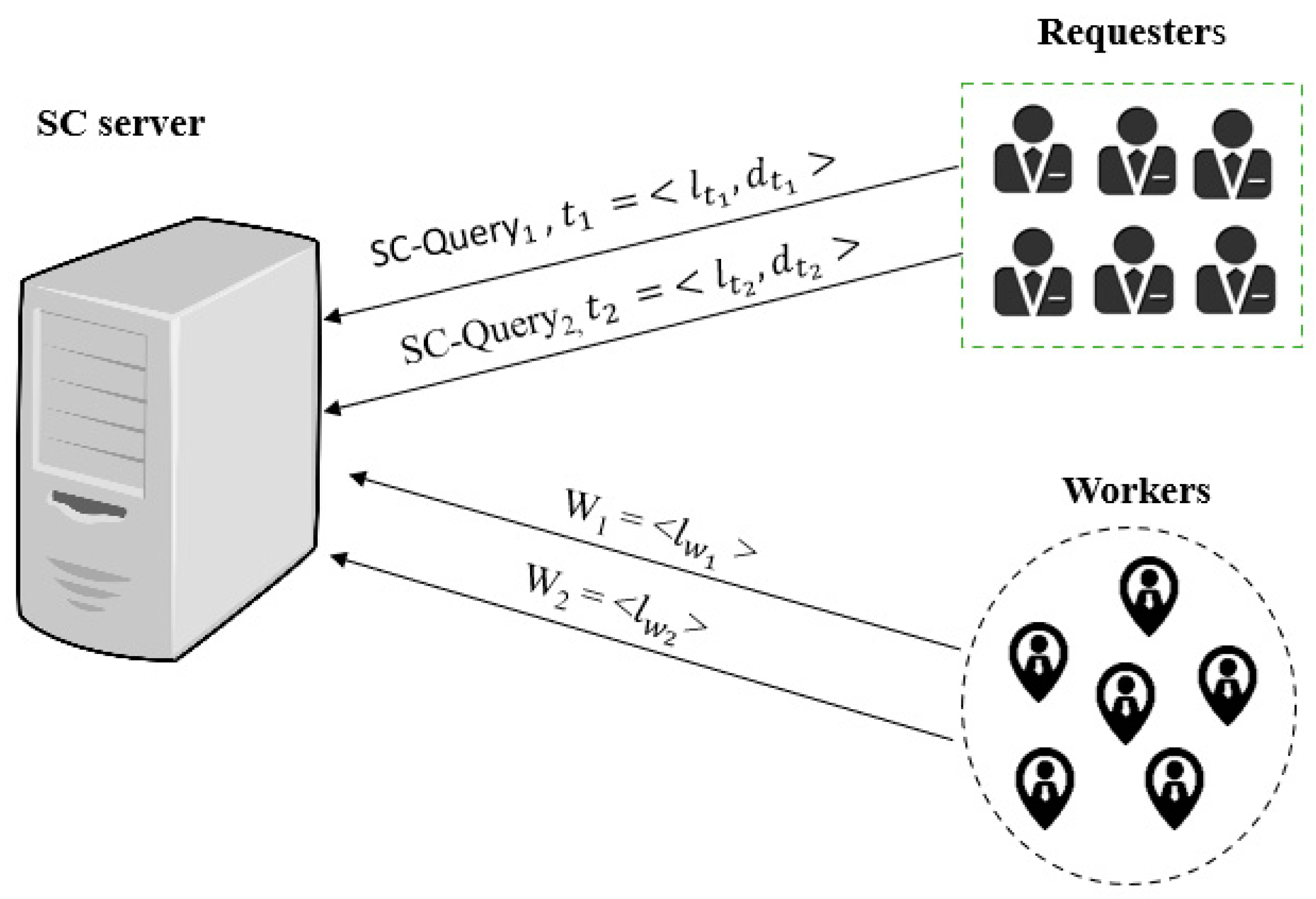
3. The MOTSO Model in SC

The MOTSO model was designed based on the integration of two main algorithms to realize the primary objectives of the research. The main procedure of our model is illustrated in Figure 3; the model starts with the ranking strategy algorithm, then utilizing the MOPSO algorithm. The following sections explain these algorithms in detail.

Figure 3. The procedure of the multi-objective task scheduling optimization (MOTSO) model. TED = task execution duration table; TE = task entropy table; RTED = ranked TED; RTE = ranked TE; w1 = first worker; w2 = second worker; w3 = third worker; t1 = first task; t2 = second task.

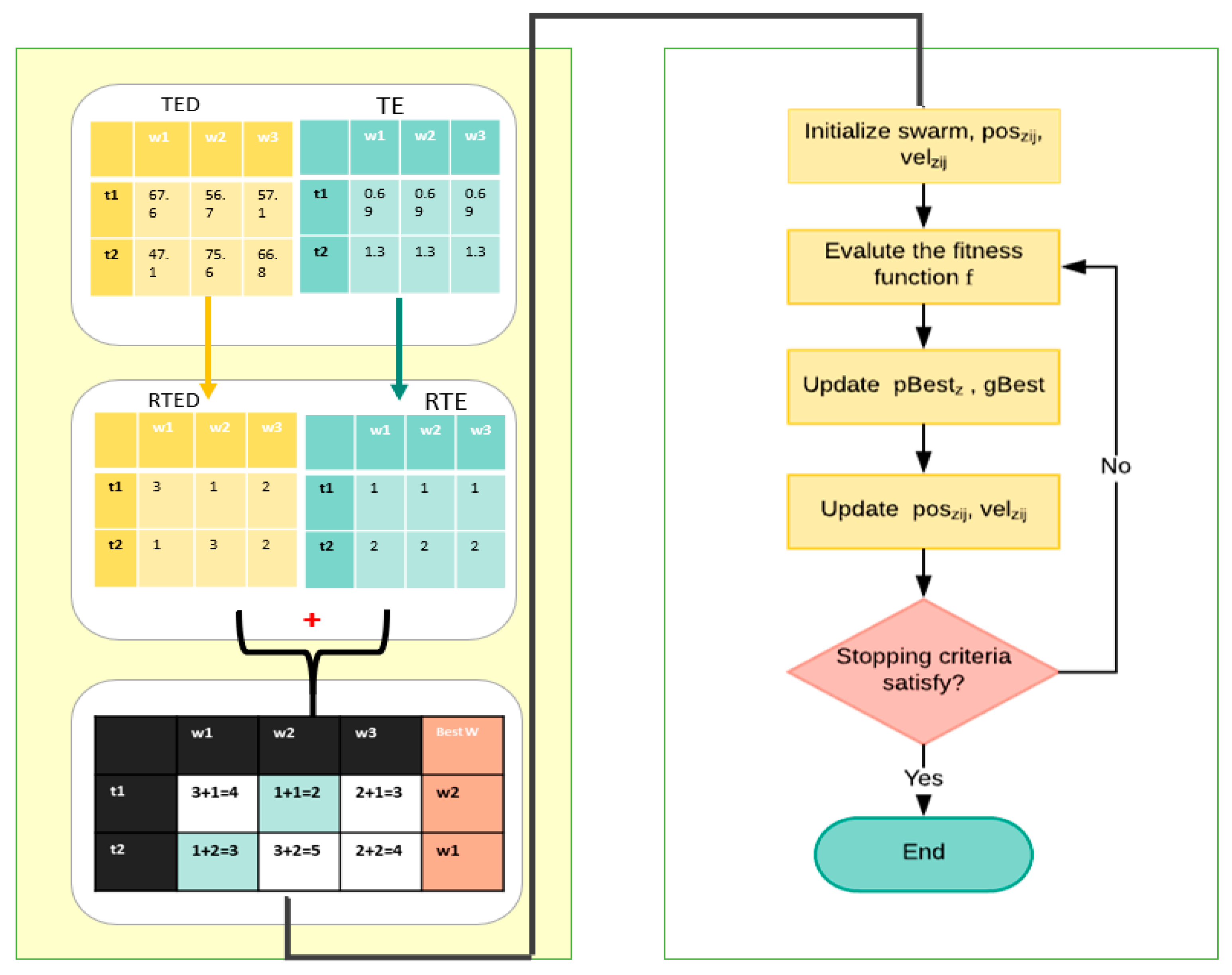
3.1. The Ranking Strategy Algorithm

The ranking strategy in our work is the pre-computation in our model. It aims to enhance the performance of our MOPSO algorithm [19]. Due to a huge search space that consists of thousands of available workers and spatial tasks where the initial particles are produced randomly, it is unlikely to be close to the optimal solution or to have it satisfying convergence performance. Thus, we improved our MOPSO model by utilizing the output solutions of this pre-computation phase (the ranking strategy) to initialize the position of the swarm directly.

Generally, the ranking strategy algorithm begins with generating both a task execution duration (TED) table and a task entropy (TE) table to construct a ranked table that determines the optimal worker (who has the least value) for each task.

Algorithm 1 describes the pre-computation stage, which starts by computing the TED and TE, as shown in lines 5–11. The computational results of these steps are stored in two different tables. After that, the TED and TE are sorted and ranked into tables (RTED and RTE) according to the lines 12 and 13. Then, these two ranked tables are combined into a ranked table to select the optimal workers for each task, as presented in Algorithm 1 (lines 14–20).

Algorithm 1. Pseudo code for algorithm pre-computation.

// Pre-computation

Input:   set of tasks T and set of workers W

Output:

Initialize TE, TC, TED, RTED, RTE, Ranked with size [|T|][|W|]

Foreach task do

Foreach worker do

= computeTC(t,w) // compute travel duration using (1).

= computeTED (t,w) // compute task execution duration using  (2).

=  computeTE(t,w) // compute task entropy using (3).

End Foreach

End Foreach

RTED = Rank(TED); // sort ascending and rank each worker for each task.

RTE = Rank(TE); // sort ascending and rank each task for each worker

Foreach task do

Foreach worker  do

=  +

End Foreach

End Foreach

= Rank () //sort ascending and rank

Return

3.1.1. Task Execution Duration (TED) and Ranked Task Execution Duration (RTED)

The TED refers to the required duration for the worker to arrive at the task’s location and to complete it. The TED can be computed by summing the execution duration (task duration) $d_{t_j}$ with traveling duration $T{C}_{ij}$, while the traveling duration can be computed by dividing the distance between the worker and the task by the speed of worker, as per the following equation:

$$T{C}_{ij}= \left(\frac{cost\left(w_i,t_j\right)}{s_{w_i}}\right), t_j\in T and w_i\in W$$

(1)

where $cost\left(w_i,t_j\right)$ is the travel cost between worker $w_i$ and task $t_j$, divided by the speed of the worker $s_{w_i},$ where the speed of the worker parameter is application-dependent.

$$TED \left(i, j\right)={ d}_{t_j}+ T{C}_{ij},\hspace{1em}{t}_j\in T and w_i\in W$$

(2)

where $d_{t_j}$ is the duration time of the task $t_j$, and $T{C}_{ij}$ is the traveling duration spent by the worker $w_i$ to arrive at the task’s location $t_j$.

Practically, the TED table is represented as an i × j matrix, where i and j indicate the number of tasks and the number of workers, respectively. The TED is computed between each worker and task using Equation (2). Then, we ranked the TED values for all of the tasks according to the least value of each row i (task) by sorting the workers into ascending order to select a suitable worker for each task, as presented in Table 2 and Table 3. The reason behind sorting the workers in an ascending order is to correspond the travel cost minimization objective. Thus, the allocation of a worker to a certain task is based on a smaller TED value, which will help to improve and minimize the travel costs. In other words, the best worker to execute a specific task is the closest one to the task’s location and the faster one in terms of task execution duration. Further, we need to sort the task’s entropies because they affect the task execution [12]. More details about the ranking of tasks entropy are provided in the next section.

Table 2. Task execution duration (TED).

	w1	w2	w3	w4	w5
t1	137.5286391016494	140.77934794265565	140.83953070394318	132.77599556103092	156.88627234146358
t2	47.12959736369906	85.88725867729572	75.65173447900676	77.63439324242962	66.8175097791553
t3	92.55306850854014	130.09070678927753	92.66485742716874	101.97479734391655	88.3209190565524

Table 3. Ranked task execution duration (RTED).

	w1	w2	w3	w4	w5
t1	2	3	4	1	5
t2	1	5	3	4	2
t3	2	5	3	4	1
t4	1	2	3	5	4

3.1.2. Task Entropy (TE) and Ranked Task Entropy (RTE)

Considering the popularity of location entropy is useful for maximizing task assignment [12]. Location entropy takes into consideration the number of visitors (workers in our case) to a particular location. In other words, if the location is visited by few workers, then each task within this location should be given a higher priority to be assigned first, because any task with a little entropy has a lower chance to be completed in the next iteration. In our study, the space was represented as 2D cells called a grid; the entropy of the cells was computed and stored in historical data in order to allow for real-time task scheduling, i.e., to reduce the time for recalculating the location entropy every time.

The TE table was structured as a i × j matrix, where i is the number of tasks and j is the number of workers (Table 4). Thus, to compute the entropy of the task, we divided the 2D map into several cells; then, we calculated the entropy for each cell based on worker occurrence, as in Equation (3). Then, the incoming tasks took the cell’s entropy value in which they appeared.

$$TE \left(t\right)=-{\displaystyle \sum }_{w\in W_t}{P}_t\left(w\right)log{P}_t\left(w\right)$$

(3)

where $W_t$ is a set of distinct users that visited location of task t, $P_t\left(w\right)$ is the probability of visits to a task location t that belongs to user $w$, and $P_t\left(w\right)=\frac{\left|O_{w,t}\right|}{\left|O_t\right|}$. Meanwhile, $\left|O_t\right|$ indicates the number of the visits to a task location in the O_t set, while $\left|O_{w,t}\right|$ indicates the number of visits of the same worker to a task location in the O_w,t set.

Table 4. Task entropy (TE).

	w1	w2	w3	w4	w5
t1	0.6931471805599453	0.6931471805599453	0.6931471805599453	0.6931471805599453	0.6931471805599453
t2	0.0	0.0	0.0	0.0	0.0
t3	1.386943611198906	1.386943611198906	1.386943611198906	1.386943611198906	1.386943611198906
t4	0.6931471805599453	0.6931471805599453	0.6931471805599453	0.6931471805599453	0.6931471805599453

After that, we ranked the TE table according to the task’s entropy value by sorting the tasks in ascending order so as to first select the task with the smallest entropy, as shown in Table 5. The reason behind sorting the tasks in ascending order was to correspond to first objective, i.e., maximizing the number of completed tasks; therefore, we give the highest priority to the task with the smallest entropy to help maximize the number of completed tasks.

Table 5. Ranked task entropy (RTE).

	w1	w2	w3	w4	w5
t1	2	2	2	2	2
t2	1	1	1	1	1
t3	4	4	4	4	4
t4	3	3	3	3	3

3.1.3. The Ranked Tables

In this step, the RTED and the RTE tables were summed into a new ranked table to select the optimal workers (who have the lowest values) for each task, as shown in Table 6. All of the shaded cells in Table 6 represent the best solution.

Table 6. Ranked table.

	w1	w2	w3	w4	w5	The Optimal Worker
t1	2 + 2 = 4	3 + 2 = 5	4 + 2 = 6	1 + 2 = 3	5 + 2 = 7	w4
t2	1 + 1 = 2	5 + 1 = 6	3 + 1 = 4	4 + 1 = 5	2 + 1 = 3	w1
t3	2 + 4 = 6	5 + 4 = 9	3 + 4 = 7	4 + 4 = 8	1 + 4 = 5	w5
t4	1 + 3 = 4	2 + 3 = 5	3 + 3 = 6	5 + 3 = 8	4 + 3 = 7	w1

To clarify further, we explain here our ranking strategy through a real example. We ran the ranking strategy algorithm with only five workers and four tasks. Table 2 presents the results of the TED between each task and worker, computed using Equation (2). For each task (row), the algorithm sorted the workers in ascending order based on the TED value. For example, for t1, w4 had the smallest TED value; thus, it took the value of 1 in the RTED table. Then, w1 = 2, w2 = 3, w3 = 4, and w5 = 5. This was done for each task until completing the RTED table. Table 4 shows the results of the TE computed for each task using Equation (3). For each column, the algorithm sorted the tasks in ascending order according to the smallest TE value. For instance, t2 had the smallest entropy value, so it took the value of 1 in the RTE table. Then, t1 = 2, t4 = 3, t3 = 4, etc. After that, RTED and RTE were summed to the ranked table, as shown in Table 6. In our example, the optimal worker for task 1 (t1) was worker 4 (w4), because his ranked value was 3 (where 1 + 2 = 3), which is the smallest compared to the other workers, and so on.

In our study, we introduced task completion priority; this means that if the optimal worker has more than one task, the worker must complete the task that has the smaller value compared to the other tasks assigned to them. Two reasons behind giving the task (with a smaller ranked value) a higher priority for completion is to reduce the total travel costs—in that the worker moves first to the closest task—and to ensure the completion of the task that has the lower entropy because higher priority is given to the task that has the lowest entropy in TE, as shown in Table 4 and as we mentioned earlier.

For more clarification, in Table 6, w1 has t2 and t4, meaning the worker must start by completing t2 then t4 because the ranked value of t2 is equal to 2, which is less than the ranked value of t3, which is equal to 4. After completing the ranked table and finding an optimal worker for each task, the MOPSO starts by utilizing this ranked table as a position of all particles, instead of randomly initializing a position of particles. The next section presents our MOPSO.

3.2. Multi-Objective Particle Swarm Optimization

MOPSO consists of several significant steps included in each iteration, as shown in Figure 4. The MOPSO algorithm starts with initializing the swarm, velocity, position, and PBestz values. The velocity of all particles is initialized randomly. Due to the huge search space (i.e., the thousands of available workers and spatial tasks), we propose utilizing the output solutions of the pre-computation phase to initialize the position of the swarm directly. We used the ranked table values as the position of the particles at the first iteration to enhance the MOPSO’s capability for achieving satisfying solutions, through accelerating the convergence effectively and to be close to the global target instead of the local target. The steps of our MOPSO and the fitness function were explained in more detail in our previous study [19].

Figure 4. Flowchart of the multi-objective particle swarm optimization (MOPSO) [19].

4. Performance Evaluation

The overall adopted algorithms were tested as one unit to evaluate the effectiveness of the MOTSO model. We implemented the proposed model using a Java environment, conducted on an Intel(R) Core(TM) i9-8950 CPU @2.90 GHz with 32 GB RAM(Intel Corporation, Santa Clara CA, USA). We used both a synthetic dataset (SYN) with SCAWQ and a real dataset (Gowalla) to test and compare our proposed model to the state-of-the-art algorithms. We generated synthetic data with uniformly (UNI) distributed grids (200 × 200). According to the synthetic dataset, we defined two different cases: the first case (case 1) with 600 independent spatial tasks and 600 workers, and the second case with 1200 workers and 1200 independent spatial tasks. Moreover, the Gowalla check-in dataset in our experiment [36] did not include tasks; thus, in our examination, we selected 2400 tasks and workers randomly from Gowalla venues by SCAWG with random task durations, as per [4]. The parameter settings used to implement our model are illustrated in Table 7. It should be noted that varying some of our model parameters (e.g., population number (P), iteration number (I), and duration max (D)) led to different results. Finally, we ran each experiment 10 times and calculated the average value for each factor.

Table 7. Experimental settings.

	Parameter	Parameter Value
MOPSO configuration	P	50
	I	80
	N	[0,1]
	C1, C2	2.00, 2.00
	r1, r2	[0,1]
SC configuration	No.w	Case1 = 600 Case2 = 1200 Gowalla = 2400
	No.t	Case1 = 600 Case2 = 1200 Gowalla = 2400
	S	80
	D	90

In this section, the test results include both the synthetic dataset (with the two cases mentioned previously) and the real dataset (Gowalla). Then, we compared our proposed model with several algorithms to evaluate the effectiveness of the MOTSO model. In Section 4.1, we present the results and discuss the ranking strategy in more detail; in Section 4.2, we present and discuss the results of the proposed MOTSO model based on our three conflicting objectives, as presented in Section 4.2.1, Section 4.2.2 and Section 4.2.3.

In Table 7:

• N is the inertia weight;
• P is population number;
• I is iteration number;
• D is duration max;
• C1 and C2 are acceleration coefficients;
• r1 and r2 are random numbers;
• S is the speed of workers;
• No.w is the number of workers;
• No.t is the number of tasks.

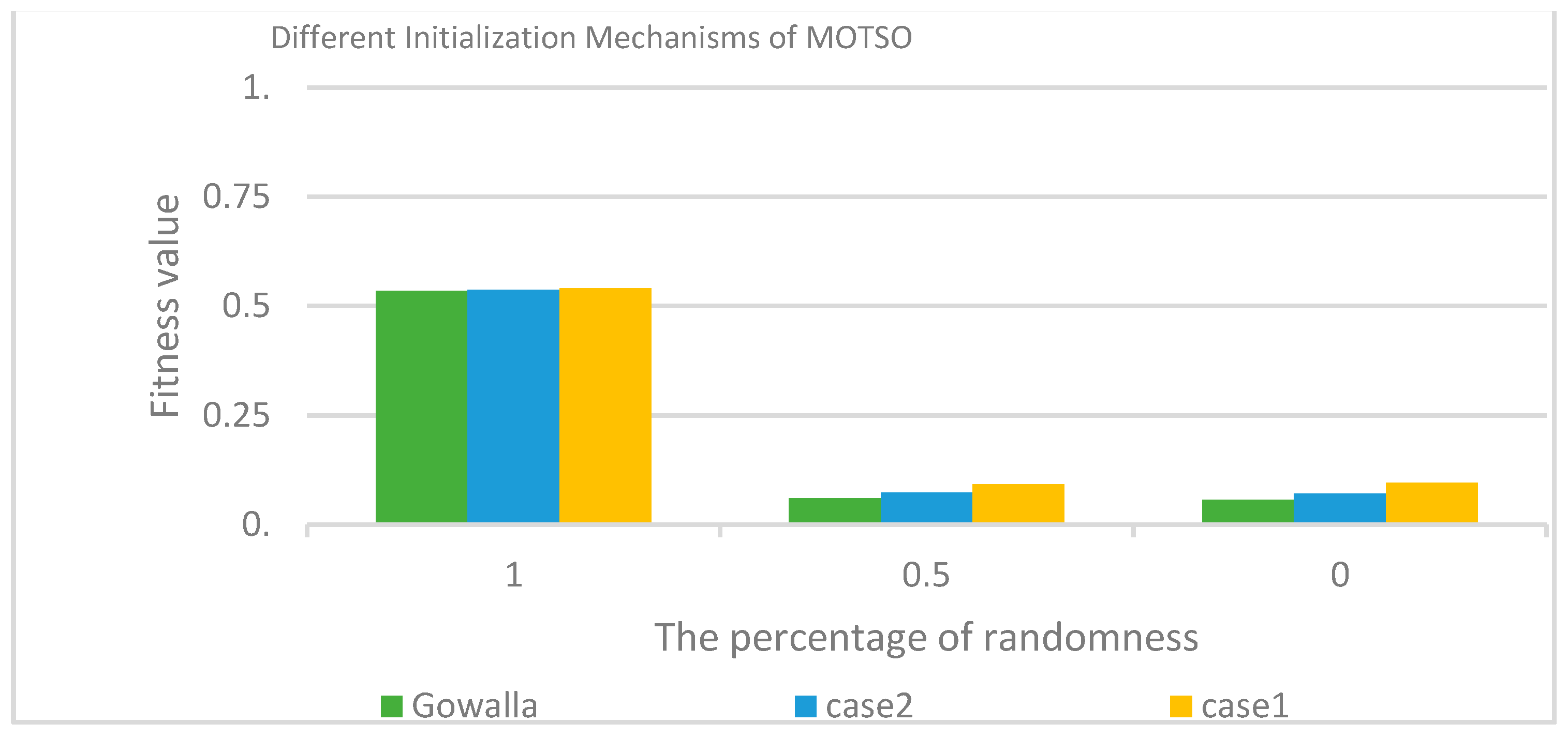
4.1. The Performance of the Ranking Strategy Algorithm

The primary purpose of employing the ranking strategy stage in our model was to enhance the performance of the MOPSO based on the primary objectives of our research. We examined the performance of our model and the impact of the ranking strategy stage on the fitness value by varying the three initialization mechanisms of the positions of the particles in the first iteration under the same parameters, and by randomly initializing the velocity of all particles. The following are the initialization mechanisms of the particles’ positions:

• Initializing the position of a particle randomly (the percentage of randomness is 100%);
• Initializing the position of a hybrid particle, both randomly and from the ranked table (the percentage of randomness is 50%);
• Initializing the positions of all particles from the ranked table (the percentage of randomness is 0%).

The fitness function value was computed using Equation (4), as mentioned in our study [19]:

$$f=NTTC+NWLB+\left(1-NV\right)$$

(4)

where $NTTC$ is the normalized TTCs, $NWLB$ is the normalized WLB, and NV is the normalized |V|. Meanwhile, $\left(1-NV\right)$ is the reverse of NV, meaning that we converted the objective of maximizing the number of completed tasks into another form—that is, minimizing the number of uncompleted tasks—in order to unify the direction of the optimization of our objectives. The results of the fitness function values are presented in Table 8.

Table 8. The results of the fitness function values when varying the initialization mechanisms.

Dataset	Fitness Function Value
	100% (Randomly)	50% (Hybrid)	0% (Ranked table)
Case 1	0.540143	0.092286	0.096544
Case 2	0.537479	0.073181	0.071633
Gowalla	0.535224	0.060976	0.056781

In more detail, we investigated the variation of the three initialization mechanisms on each objective (i.e., the number of completed tasks, the total travel costs, and the balance of workers’ workload). It should be noted that in the fitness function, we reversed the maximizing the number of completed tasks objective to a new form, i.e., minimizing the number of uncompleted tasks objective. In order to unify the direction of all objectives in terms of “minimizing”, in Table 9 we display the results of $1-NV$, which is the number of uncompleted tasks, as well as the normalized TTCs (NTTCs) and the normalized workload balance (NWLB).

Table 9. Normalization values of the objectives in terms of minimization when varying the initialization mechanisms.

	Normalization Values for Each Objective in Terms of Minimization
	$1-\mathit{N}\mathit{V}$			NWLB			NTTC
	100%	50%	0%	100%	50%	0%	100%	50%	0%
Case 1	0.34853	0.026923	0.034188	0.039943	0.048828	0.051251	0.15167	0.016535	0.011105
Case 2	0.35715	0.026961	0.027024	0.028998	0.034157	0.036681	0.151331	0.012063	0.007929
Gowalla	0.365401	0.026474	0.024522	0.020456	0.024455	0.026705	0.149367	0.010047	0.005554

Table 8 and Table 9 show the evaluation of using the ranking strategy and its impact on the performance of our proposed model. Figure 5 illustrates that there are no essential differences between the performance of the proposed MOTSO model when setting the percentage of randomness to 0% or 50%. Thus, we focused on only two of initialization mechanisms:

Figure 5. The fitness value when varying the initialization mechanisms.

• Initializing the positions of all particles randomly;
• Initializing the positions of all particles using the output of the ranking strategy stage.

Figure 5 shows that using the output of the ranking strategy as the particle’s position in the first iteration (the percentage of randomness is 0%) improves the fitness value to approximately 82% and 86% in case 1 and case 2, respectively, and to approximately 89% in the real dataset compared to initializing the positions of all particles randomly. Due to the huge search space included in our research (i.e., consisting of hundreds or thousands of available workers and spatial tasks), the ranking strategy improves the convergence of the particles to the best solution regarding the objectives of the MOTSO model.

There is a big difference in both the number of completed tasks and the total travel costs, as shown in Figure 6, when the positions of all particles are initialized from the output of the ranking strategy in the first iteration, as mentioned in Section 3.

Figure 6. The percentages of completed tasks using the proposed MOTSO model for case 1 (a), case 2 (b), and Gowalla (c).

The number of completed tasks can be improved by the ranking strategy to approximately 90% in case 1, 92% in case 2, and 93% in Gowalla. The total travel costs can be reduced when using the ranking strategy to approximately 93%, 95%, and 96% in case 1, case 2, and Gowalla, respectively, compared to the random initialization of particles under the same parameter settings. Otherwise, there are no important differences in WLB. The reason behind these improvements in only two objectives is because the ranking strategy contains two main tables. The first table is the TED table, which positively affects the reduction of travel costs, where the best worker is selected to perform a specific task based on who is closest to this task’s location. The second table is the TE table, where the task entropy helps to maximize the number of completed tasks.

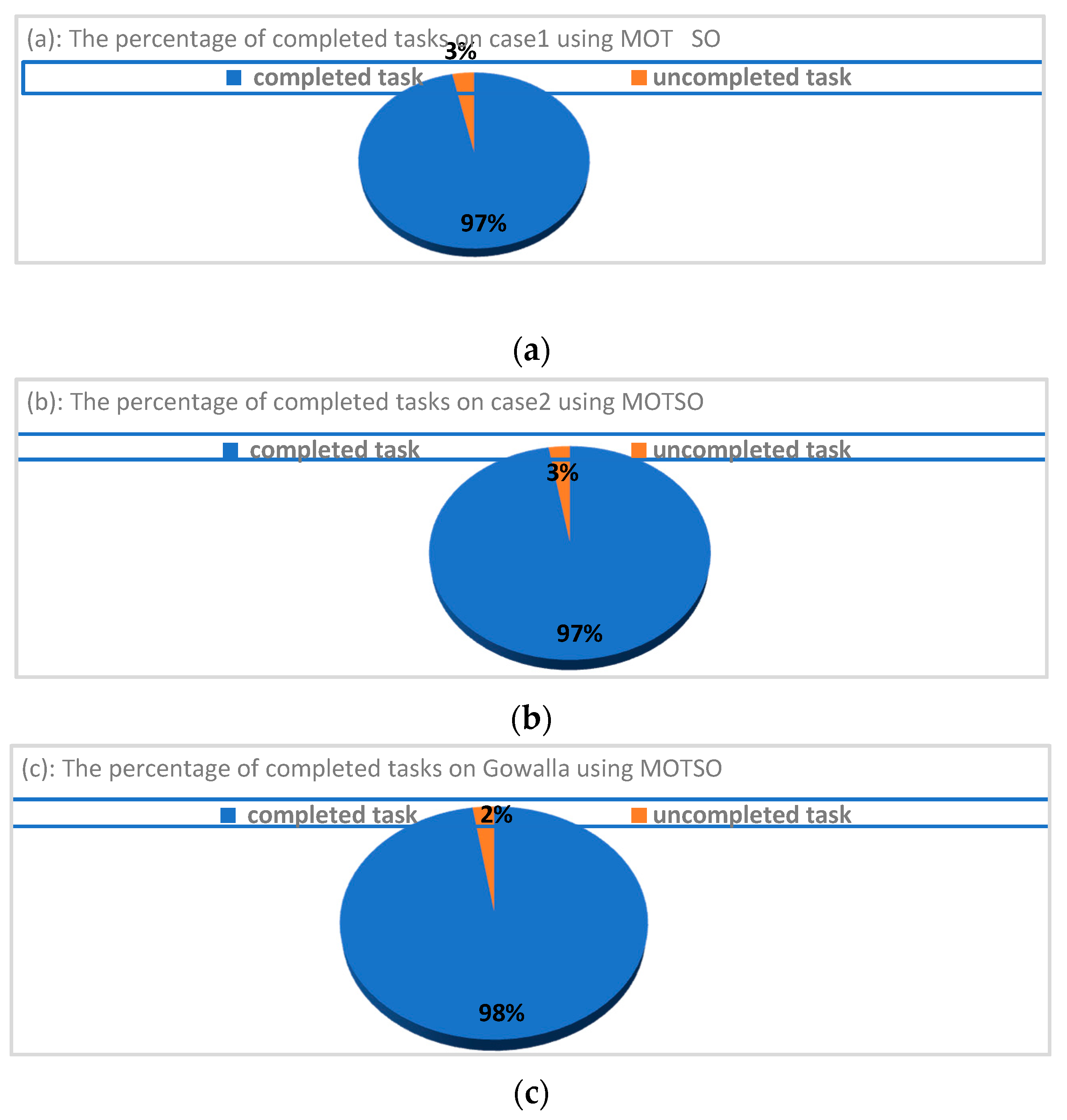
4.2. Performance of the MOTSO Model

The proposed model aims to maximize the number of a completed tasks, as well as to minimize the TTCs and to ensure the balance of the workload between workers. Here, we present the detailed results of using the MOTSO model based on the MOPSO algorithm, and we discuss the findings for each research objective in the following sections.

4.2.1. Maximizing the Number of Completed Tasks

According to the first objective, i.e., maximizing the number of completed tasks, Table 10 shows the results of the number of tasks achieved using our proposed model in the synthetic dataset (with two cases) and the Gowalla dataset; |V| and |T| indicate the number of completed tasks and the total number of tasks in the task set, respectively. Indeed, there are no differences in the performance of MOTSO between the synthetic dataset (in two cases) and the real dataset, that is, the performance of our proposed solution was compared by the different algorithms mentioned in related works [2,10], in terms of the number of completed tasks using the Gowalla dataset.

Table 10. The result of the total travel costs (TTCs) using our MOTSO model.

Dataset	Total Travel Cost Using MOTSO
	TTCs
Case 1	637.2025
Case 2	917.3457
Gowalla	1292.929

The percentages of the completed tasks are presented in Figure 7, where our MOTSO model achieved the highest percentage of completed tasks, reaching approximately 98% compared to the other algorithms (i.e., baseline algorithm (A&S), global assignment and local scheduling algorithm (GALS), naïve local assignment local scheduling based on location (NLALA-L), naïve local assignment local scheduling based on task-oriented partitioning (NLALS-T), bisection-based local assignment and local scheduling based on K-means (BLALS-K), bisection-based local assignment and local scheduling based on task-oriented partitioning (BLALS-T), baseline algorithm (BLA), load-balancing algorithm (LBA), and the divide-and-conquer algorithm (DCA)) in [2,10]. In other words, the performance of the proposed MOTSO was better than that of the other methods, as illustrated in Figure 7. Based on this, our MOTSO model achieved effective performance regarding the first objective of the MOTSO model, i.e., maximizing the number of completed tasks, because we adapted the MOPSO based on a fitness function that considers the number of completed tasks in each iteration, which helped to improve and increase the number of completed tasks. Additionally, consideration of the task entropy in the ranking strategy algorithm helped to maximize the number of completed tasks.

Figure 7. The percentage of completed tasks using different algorithms. A&S = baseline algorithm; GALS = global assignment and local scheduling algorithm; NLALA-L = naïve local assignment local scheduling based on location; NLALS-T = naïve local assignment local scheduling based on task-oriented partitioning; BLALS-K = bisection-based local assignment and local scheduling based on K-means; BLALS-T = bisection-based local assignment and local scheduling; BLA = baseline algorithm; LBA = load-balancing algorithm; DCA = divide-and-conquer algorithm.

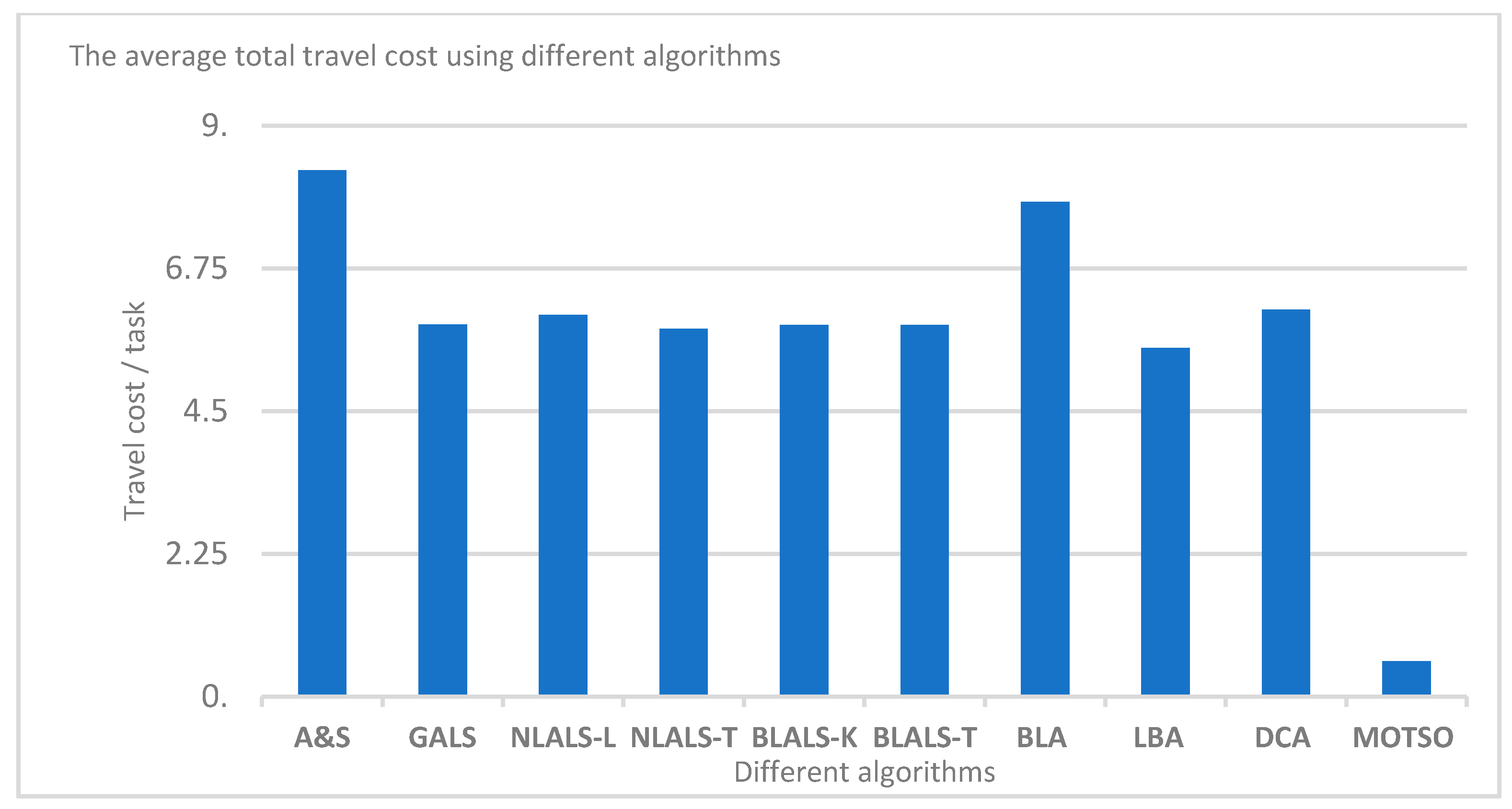
4.2.2. Minimizing the Total Travel Costs (TTCs)

The TTCs are a fundamental component, given the nature of the moves taken by a worker from one location to another in order to achieve spatial tasks. Table 10 presents the total travel costs achieved by the proposed model.

The effectiveness of the MOTSO model in terms of the minimizing the total travel cost objective was compared with the different algorithms mentioned in [2,10] using only the Gowalla dataset because there were no differences between the MOTSO results between the synthetic and real datasets. In order to conduct the comparison, we calculated the average TTC (i.e., the ratio of total travel costs per number of completed tasks using the equation mentioned in our previous work [19]):

$$Average Travel Cost \left(ATC\right)= \frac{TTC}{\left|V\right|}$$

(5)

where TTC is the total travel cost and |V| is the number of completed tasks $v_{ij}$. The results of the average travel cost (ATC) using the Gowalla dataset for all algorithms are presented in Table 11.

Table 11. The results of the average travel cost (ATC) using different algorithms.

Using Gowalla
Name of algorithm	ATC value
A&S	8.30
GALS	5.87
NLALA-L	6.02
NLALS-T	5.80
BLALS-K	5.86
BLALS-T	5.86
BLA	7.8
LBA	5.5
DCA	6.1
MOTSO (our model)	0.5527457

Figure 8 illustrates that the proposed MOTSO model outperforms all of the methods regarding minimizing the average travel cost per task, i.e., the results of the experiment validate the effectiveness of the MOTSO model in terms of minimizing the total travel costs. The reason behind this outperformance in the TTC objective is the application of the TED table in selecting the best worker (who is the closest to the task’s location) to perform a specific task, as well as the task completion priority, where the same worker starts with the nearest task firstly in their schedule.

Figure 8. The average total travel cost using different algorithms.

4.2.3. Minimizing the Standard Deviation of the Workload Balance

In our model, the workload for each worker was the traveled distance plus the duration of the execution time for the tasks done by the same worker, as calculated in [19].

We considered the standard deviation as a metric to quantify the workload between all workers because the decreased standard deviation of the worker’s workload helps to prevent overloading between the workers. Table 12 shows the standard deviation of the workload balance results using the MOTSO model.

Table 12. The results of the standard deviation of the workload balance (WLB) using the MOTSO model.

Dataset	Workload Balancing Using MOTSO
	WLB
Case 1	55.58566
Case 2	56.42424
Gowalla	58.01609

The baseline in our work was the approach introduced in [2]. We compared the MOTSO using the BLA to evaluate the effectiveness of our model according to the workload balance objective under the same experimental settings. Moreover, we computed the standard deviations of workload balance for the two algorithms, i.e., the BLA and our MOTSO model. Furthermore, we conducted a statistical test to compare the two different standard deviation values; for this, we selected t (independent-samples t-test).

Regarding the synthetic dataset (case 1), there was a significant difference in the scores for the BLA (M = 184.1136, SD = 47.17132) and our MOTSO model (M = 44.32074, SD = 55.58566); where the value of t (1198) = 46.9692 and p = 0.0001. These results show that our MOTSO model is able to reduce the workload of a worker compared to the BLA. In case 2, the score of the BLA was M = 185.4424 and SD = 45.72034, while the score of our BLA was M = 44.411495 and SD = 56.424235; based on the t-value (2398) being 67.2718 (p = 0.0001), there was a significant difference in the scores for the BLA and MOTSO in case 2. These results indicate that our model can improve the workload of workers.

According to the results of the real dataset (Gowalla), the BLA score was M = 182.2911 and SD = 48.25323 and that of our MOTSO was M = 44.339762 and SD = 58.016085, where t-value (4798) = 89.5599 and p = 0.0001. There was a significant difference between the results of the two algorithms, where the workload of the worker decreased more with our MOTSO model.

Based on the previously mentioned results of an independent-samples t-test, p > 0.05 in both the synthetic dataset and the Gowalla dataset, so there was a significant difference between the two algorithms in terms of minimizing the standard deviation of the workload balance, which is in favor of our model. In other words, our model improves the workload balance between all workers compared to the BLA. Thus, our MOTSO model is effective in regard to the load balancing objective.

5. Conclusions

Recently, a new framework referred to as spatial crowdsourcing (SC) was introduced to achieve spatial tasks in a crowdsourcing environment. However, there are many challenges in SC, with the core one being task assignment, formulated as the task matching or task scheduling problem.

Task scheduling is an important issue, where the worker can view their trajectories to complete all tasks that are assigned to them. In real applications, SC usually requires optimizing several objectives, many of which may be conflicting. However, there is a lack of studies that address the multi-objective optimization problem, as well as the task scheduling problem, within an SC environment.

In this study, we focused on the TS-MOO issue in SC, which aims to maximize the number of completed tasks, minimize the total travel costs, and ensure the balance of the workload between workers. To solve this issue, we proposed a new MOTSO model to find the optimal task scheduling approach based on three conflicting objectives. The MOTSO model includes a modification of two main algorithms related to fitness function and the ranking strategy to enhance its performance.

We conducted experiments to evaluate the proposed method using a synthetic and a real dataset. The extensive results and statistical analyses showed that our proposed model proved effective in terms of maximizing the number of completed tasks, minimizing the total travel costs, and ensuring the balance of the workload between workers.

As regards future work, we plan to extend our model to deal with complex tasks that require multiple workers to finish one task. Additionally, we plan to extend our model to deal with heterogeneous tasks in SC.

References

1. Wang, Y.; Jia, X.; Jin, Q.; Ma, J. Mobile crowdsourcing: Framework, challenges, and solutions. Concurr. Comput. Pr. Exp. 2016, 29, e3789. [Google Scholar] [CrossRef]
2. Sun, D.; Gao, Y.; Yu, D. Efficient and Load Balancing Strategy for Task Scheduling in Spatial Crowdsourcing. In Web-Age Information Management; Song, S., Tong, Y., Eds.; Springer: Berlin, Germany, 2016; pp. 161–173. [Google Scholar]
3. Tong, Y.; She, J.; Ding, B.; Wang, L.; Chen, L. Online mobile Micro-Task Allocation in spatial crowdsourcing. In Proceedings of the 2016 IEEE 32nd International Conference on Data Engineering (ICDE), Helsinki, Finland, 16–20 May 2016; pp. 49–60. [Google Scholar]
4. Song, T.; Tong, Y.; Wang, L.; She, J.; Yao, B.; Chen, L.; Xu, K. Trichromatic Online Matching in Real-Time Spatial Crowdsourcing. In Proceedings of the 2017 IEEE 33rd International Conference on Data Engineering (ICDE), San Diego, CA, USA, 19–22 April 2017; pp. 1009–1020. [Google Scholar]
5. Zhao, Y.; Han, Q. Spatial crowdsourcing: Current state and future directions. IEEE Commun. Mag. 2016, 54, 102–107. [Google Scholar] [CrossRef]
6. Kazemi, L.; Shahabi, C. GeoCrowd: Enabling Query Answering with Spatial Crowdsourcing. In Proceedings of the 20th International Conference on Intelligent User Interfaces, Redondo Beach, CA, USA, 6–9 November 2012; pp. 189–198. [Google Scholar]
7. Chen, L.; Shahabi, C. Spatial Crowdsourcing: Challenges and Opportunities. IEEE Data Eng. Bull. 2016, 39, 14–25. [Google Scholar]
8. Cheng, P.; Lian, X.; Chen, L.; Han, J.; Zhao, J. Task Assignment on Multi-Skill Oriented Spatial Crowdsourcing. IEEE Trans. Knowl. Data Eng. 2016, 28, 2201–2215. [Google Scholar] [CrossRef]
9. Kazemi, L.; Shahabi, C.; Chen, L. GeoTruCrowd: Trustworthy Query Answering with Spatial Crowdsourcing. In Proceedings of the 21st ACM SIGSPATIAL International Conference on Advances in Geographic Information Systems, Orlando, FL, USA, 5–8 November 2013; pp. 314–323. [Google Scholar]
10. Deng, D.; Shahabi, C.; Zhu, L. Task matching and scheduling for multiple workers in spatial crowdsourcing. In Proceedings of the 23rd SIGSPATIAL International Conference on Advances in Geographic Information Systems, Seattle, DC, USA, 3–6 November 2015; p. 21. [Google Scholar]
11. Deng, D.; Shahabi, C.; Demiryurek, U. Maximizing the number of worker’s self-selected tasks in spatial crowdsourcing. In Proceedings of the 21st ACM SIGSPATIAL International Conference on Advances in Geographic Information Systems, Orlando, FL, USA, 5–8 November 2013; pp. 324–333. [Google Scholar]
12. Tran, L.; To, H.; Fan, L.; Shahabi, C. A Real-Time Framework for Task Assignment in Hyperlocal Spatial Crowdsourcing. ACM Trans. Intell. Syst. Technol. 2018, 9, 1–26. [Google Scholar] [CrossRef]
13. Tsai, J.-T.; Fang, J.-C.; Chou, J.-H. Optimized task scheduling and resource allocation on cloud computing environment using improved differential evolution algorithm. Comput. Oper. Res. 2013, 40, 3045–3055. [Google Scholar] [CrossRef]
14. Zhang, G.; Zuo, X. Deadline Constrained Task Scheduling Based on Standard-PSO in a Hybrid Cloud. In Advances in Swarm Intelligence; Tan, Y., Shi, Y., Mo, H., Eds.; Springer: Berlin/Heidelberg, Germany, 2013; Volume 7928, pp. 200–209. [Google Scholar]
15. Jana, B.; Chakraborty, M.; Mandal, T. A Task Scheduling Technique Based on Particle Swarm Optimization Algorithm in Cloud Environment. In Soft Computing: Theories and Applications; Ray, K., Sharma, T.K., Rawat, S., Saini, R.K., Bandyopadhyay, A., Eds.; Springer: Singapore, 2019; Volume 742, pp. 525–536. [Google Scholar]
16. Kennedy, J.; Eberhart, R. Particle swarm optimization. In Proceedings of the ICNN’95-International Conference on Neural Networks, Perth, WA, Australia, 27 November–1 December 1995; Volume 4, pp. 1942–1948. [Google Scholar] [CrossRef]
17. Wang, D.; Tan, D.; Liu, L. Particle swarm optimization algorithm: An overview. Soft Comput. 2018, 22, 387–408. [Google Scholar] [CrossRef]
18. Coello, C.C.; Lechuga, M. MOPSO: A proposal for multiple objective particle swarm optimization. In Proceedings of the 2002 Congress on Evolutionary Computation, 2002. CEC ’02, Honolulu, HI, USA, 12–17 May 2003; Volume 2, pp. 1051–1056. [Google Scholar]
19. Alabbadi, A.A.; Abulkhair, M.F. Task-Scheduling Based on Multi-Objective Particle Swarm Optimization in Spatial Crowdsourcing. J. King Abdulaziz Univ. Comput. Inf. Technol. Sci. 2019, 8, 45–57. [Google Scholar] [CrossRef]
20. Chen, Z.; Fu, R.; Zhao, Z.; Liu, Z.; Xia, L.; Chen, L.; Cheng, P.; Cao, C.C.; Tong, Y.; Zhang, C.J. gMission: A General Spatial Crowdsourcing Platform. Proc. VLDB Endow. 2014, 7, 1629–1632. [Google Scholar] [CrossRef]
21. Uber. Available online: https://www.uber.com// (accessed on 22 November 2018).
22. Google Maps. Available online: https://www.google.com/maps (accessed on 22 November 2018).
23. Free Driving Directions, Traffic Reports & GPS Navigation App by Waze. Available online: https://www.waze.com/ (accessed on 22 November 2018).
24. Restaurants, Dentists, Bars, Beauty Salons, Doctors—Yelp. Available online: https://www.yelp.com/ (accessed on 22 November 2018).
25. TaskRabbit Connects You to Safe and Reliable Help in Your Neighborhood. Available online: https://www.taskrabbit.com/ (accessed on 22 November 2018).
26. Gigwalk: We’ve Got Your Brand’s Back—Gigwalk. Available online: http://www.gigwalk.com/ (accessed on 22 November 2018).
27. To, H. Task Assignment in Spatial Crowdsourcing: Challenges and Approaches. In Proceedings of the 3rd ACM SIGSPATIAL PhD Symposium, Burlingame, CA, USA, 31 October 2016; Volume 1, pp. 1–4. [Google Scholar]
28. Cheng, P.; Jian, X.; Chen, L. Task Assignment on Spatial Crowdsourcing (Technical Report). arXiv 2016, arXiv:1605.09675. [Google Scholar]
29. Gummidi, S.R.B.; Xie, X.; Pedersen, T.B. A Survey of Spatial Crowdsourcing. ACM Trans. Database Syst. 2019, 44, 1–46. [Google Scholar] [CrossRef]
30. Tong, Y.; Zhou, Z.; Zeng, Y.; Chen, L.; Shahabi, C. Spatial crowdsourcing: A survey. VLDB J. 2019, 29, 217–250. [Google Scholar] [CrossRef]
31. To, H.; Shahabi, C.; Kazemi, L. A Server-Assigned Spatial Crowdsourcing Framework. ACM Trans. Spat. Algorithms Syst. 2015, 1, 1–28. [Google Scholar] [CrossRef]
32. To, H.; Fan, L.; Tran, L.; Shahabi, C. Real-time task assignment in hyperlocal spatial crowdsourcing under budget constraints. In Proceedings of the 2016 IEEE International Conference on Pervasive Computing and Communications (PerCom), Sydney, NSW, Australia, 14–19 March 2016; pp. 1–8. [Google Scholar]
33. Alfarrarjeh, A.; Emrich, T.; Shahabi, C. Scalable Spatial Crowdsourcing: A Study of Distributed Algorithms. In Proceedings of the 2015 16th IEEE International Conference on Mobile Data Management, Pittsburgh, PA, USA, 15–18 June 2015; Volume 1, pp. 134–144. [Google Scholar]
34. Hassan, U.U.; Curry, E. Efficient task assignment for spatial crowdsourcing: A combinatorial fractional optimization approach with semi-bandit learning. Expert Syst. Appl. 2016, 58, 36–56. [Google Scholar] [CrossRef]
35. Wang, L.; Yu, Z.; Han, Q.; Guo, B.; Xiong, H. Multi-Objective Optimization Based Allocation of Heterogeneous Spatial Crowdsourcing Tasks. IEEE Trans. Mob. Comput. 2017, 17, 1637–1650. [Google Scholar] [CrossRef]
36. SNAP: Network Datasets: Gowalla. Available online: http://snap.stanford.edu/data/loc-gowalla.html (accessed on 17 January 2017).
Publisher’s Note: MDPI stays neutral with regard to jurisdictional claims in published maps and institutional affiliations.
Article Metrics
Citations
Article Access Statistics
Multiple requests from the same IP address are counted as one view.