Hexadecimal Aggregate Approximation Representation and Classification of Time Series Data

Abstract

Time series data are widely found in finance, health, environmental, social, mobile and other fields. A large amount of time series data has been produced due to the general use of smartphones, various sensors, RFID and other internet devices. How a time series is represented is key to the efficient and effective storage and management of time series data, as well as being very important to time series classification. Two new time series representation methods, Hexadecimal Aggregate approXimation (HAX) and Point Aggregate approXimation (PAX), are proposed in this paper. The two methods represent each segment of a time series as a transformable interval object (TIO). Then, each TIO is mapped to a spatial point located on a two-dimensional plane. Finally, the HAX maps each point to a hexadecimal digit so that a time series is converted into a hex string. The experimental results show that HAX has higher classification accuracy than Symbolic Aggregate approXimation (SAX) but a lower one than some SAX variants (SAX-TD, SAX-BD). The HAX has the same space cost as SAX but is lower than these variants. The PAX has higher classification accuracy than HAX and is extremely close to the Euclidean distance (ED) measurement; however, the space cost of PAX is generally much lower than the space cost of ED. HAX and PAX are general representation methods that can also support geoscience time series clustering, indexing and query except for classification.

1. Introduction

Time provides a basic cognitive variable for the continuity and sequential description of object movements and changes in the world [1,2,3,4,5,6]. Human society is facing many challenges, such as environmental pollution, population growth, urban expansion, the transmission of infectious diseases and various natural disaster monitoring and prevention issues, etc. These are all closely related to the concept of time and produce massive data containing information regarding time. Especially in recent years, a large amount of time series data has been produced due to the general use of smartphones, various sensors, RFID and other internet devices [2,3,4,5,6]. Time series data can help us understand history, master the present and predict the future, as well as improve our ability to gain insight, perception and prediction of the evolution of various existences and states in the real world.

Many applications in the fields of scientific research, industry and business produce large amounts of time-series data that need effective analysis, requiring rational representation and efficient similarity computing and search. These applications cover the domains of images, audio, finance, environmental monitoring and other scientific disciplines [7,8,9]. Many creative representation methods for time series data have been proposed for similarity computing, clustering [10], classification [11], indexing and query [3,8,9,12,13,14,15,16,17,18,19,20,21,22,23,24,25,26,27,28,29,30,31,32,33,34,35]. The taxonomy of time series representations includes four types [10]: data-adaptive, non-data adaptive, model-based and data dictated. The main representation methods for time series are shown in Table 1.

Table 1. Main representation methods for time series data (— no indicated by authors; n is the length of time series; T1 non-data adaptive; T2 data-adaptive; T3 data dictated; T4 model-based).

Representation Method	Year	Type	Complexity	References
Auto-regressive (AR) model	1971	T4		[36,37]
Discrete Fourier Transform(DFT)	1993	T1	O(n(log(n)))	[13,38]
Discrete Wavelet Transform (DWT)	1999	T1	O(n)	[12,39]
Singular Value Decomposition (SVD)	1997	T2		[40]
Discrete Cosine Transformation (DCT)	1997	T1	—	[40]
Piecewise Linear Approximation (PLA)	1998	T2	O(n(log(n)))	[17]
Hidden Markov models (HMMs)	1998	T4	—	[41]
Piecewise Aggregate Approximation (PAA) or Segmented Means	2000	T1	O(n)	[42]
Piecewise Constant Approximation (PCA)	2000	T2	—	[43]
Adaptive Piecewise Constant Approximation (APCA)	2002	T2	O(n)	[16]
Perceptually important point (PIP)	2001	T1	—	[44]
Chebyshev Polynomials (CHEB)	2004	T1	—	[45]
Symbolic Aggregate Approximation (SAX)	2003	T2	O(n)	[19,22]
HOT SAX	2005	T2		[46]
Clipped Data	2005	T3	—	[47]
Group SAX	2006	T2		[48]
Extended SAX	2006	T2		[49]
Combining SAX and Piecewise Linear Approximation	2007	T2		[50]
Indexable Piecewise Linear Approximation (IPLA)	2007	T1	—	[51]
1d-SAX	2013	T2		[52]
Move-Split-Merge (MSM)	2013			[53]
SAX-VSM	2013	T2		[54]
SAX-EFG	2014	T2		[55]
Tree-based Representations	2015			[56]
SC-DTW	2015	T1		[57]
Representation based on Local Autopatterns	2016			[58]
Grid Representation	2019			[59]
SAX Navigator	2019	T2		[60]
SAX-ARM	2020	T2		[61]
SAX-BD	2020	T2		[62]
Data-driven Kernel-based Probabilistic SAX	2021	T2		[63]

The most commonly used approximation representations are the PAA [42] and SAX [19,22,64] methods. In the last decades, most of time series data indexing methods [23,25,31,32,65,66] have been based on SAX [19,22]. The SAX method reduces an n-length time series to a w-length (w < n) string with an alphabet parameter named α. Though highly simple and straightforward, it is a major limitation because it may lead to some important features being lost [67]. To avoid this problem, the ESAX [68] and SAX-TD [67] methods improve the accuracy of SAX. The ESAX method adds two additional values, a maximum value and a minimum value, to each time series segment as the new feature. The mapping method between the new feature to SAX words is the same as the SAX method. Therefore, the length of the ESAX string is three times that in SAX. The SAX-TD method adds a trend distance for each segment; hence, the length of the symbol string is also two times the original string length. Therefore, both ESAX and SAX-TD methods require additional information to extend the original SAX string. The SAX-BD [62] method has a design integrating the SAX distance with a weighted boundary distance, resulting in it outperforming SAX-TD. Symbolic aggregate approximation methods have proven very effective in compacting the information content of time series. However, typical SAX-based techniques rely on a Gaussian assumption for the underlying data statistics, which often deteriorates their performance in practical scenarios [63].

To overcome this limitation, a novel method, the Hexadecimal Aggregate approXimation representation (HAX) of time series, is proposed in this paper. This method negates any assumption on the probability distribution of time series and represents each segment of a time series as a transformable interval object (TIO), using the transformation distance to measure the similarity between a pair of time series. Then, each TIO is mapped to a hexadecimal symbol by its location on a hexadecimal grid. Therefore, the HAX string is the same length as the SAX string with the same word size, the w parameter. We compare SAX, SAX-TD and SAX-BD methods with HAX methods. Our reason for choosing the SAX-TD and SAX-BD is that the outputs of the SAX-TD and SAX-BD still include the original SAX string, despite including some attachments; hence, there is comparability with the hex string of HAX. The experimental results show that HAX has higher accuracy than the SAX method. The remainder of the paper is organized as follows. Section 2 is the related work, Section 3 details the principle and method of HAX, Section 4 is the experimental evaluation and the last section is the conclusion.

2. Related Work

The most straightforward strategy for the representation of time series involves using a simple shape to reduce a segment, such as the piecewise linear representation (PLR) [17], the perceptually important point (PIP) [44] and the indexable piecewise linear approximation (IPLA) [51], among others. The simple shapes may be a point or a line. For example, the PLR and IPLA represent the original series as a set of straight lines fitting the important points of the series, and the PIP selects some important points of a segment to express the whole segment.

Another type involves choosing a simple value or symbol to express a segment of a time series. The PAA [42] method is the foundation of many time series representation methods, especially for SAX [19,22]. To reduce noise while preserving the trend of a time series, the PAA method takes the mean value over back-to-back points to decrease the number of points, as shown in Figure 1. At first, this method divides the original time series into w fixed-size segments and then computes the average values for each one. The data sequence assembled from the average values is the PAA approximation value of the original time series.

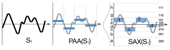
Figure 1. The relationship between PAA and SAX ([5]).

For instance, an n-length time series C is reduced to w symbols. At first, the time series is divided into w segments by the PAA method. The average value of each segment is shown as $\overline{C} = \overline{C_1}, \overline{C_2},\dots , \overline{C_w}$, in which the ith item of $\overline{C}$ is the average value of the ith segment and is computed by the Equation (1).

$$\overline{C_i}=\frac{w}{n}{\displaystyle \sum }_{j=(n/w)(i+1)+1}^{(n/w)i}{C}_j$$

(1)

here, $C_j$ is a one-time point value of the time series C.

The SAX method is one of the most typical time-series representation methods based on symbolic expression and has the same dividing strategy as the PAA method. The difference between the two is the mapping rule that the SAX uses. The SAX method divides a time series into a certain number of fixed-length subsequences (called segments) and uses symbols to represent the mean of each subsequence. There is an assumption that the time series data conforms to the Gaussian distribution, and the average value of each segment has an equal probability in the SAX. These are the base principle of the breakpoint strategy used in the SAX. This strategy makes the SAX method different from the PAA, and it can map each segment into its specified range determined by the Gaussian distribution [69]. Indeed, there is a lookup table in the SAX method with breakpoints that divide a Gaussian distribution in an arbitrary number of equiprobable regions. SAX uses this table to divide the series and map it into a SAX string [19,22], while the parameter w determines how many dimensions to reduce for the n-length time series. The smaller the parameter w is, the larger n/w is, resulting in a higher compression ratio. Finally, the SAX method can map each segment’s average value to an alphabetic symbol. The symbol string after those mappings can roughly indicate the time series.

The SAX method is well known and has been recognized by many researchers; however, the limits are also obvious. Therefore, many extended and updated methods of the SAX have been proposed, with some of the typical ones being the ESAX [67] method and the SAX-TD [66] method, among others. The ESAX method can express the more detailed features of a time series by adding a maximum value and a minimum to a new feature compared to the SAX. In addition, the SAX-TD method improves the ESAX via a trend distance strategy. The SAX-BD [4] method, proposed by us in our previous work, develops the SAX-TD using boundary distance.

3. Hexadecimal Aggregate Approximation Representation

The HAX method lets an n-length time series be reduced to w two-dimensional points in a hexadecimal plane (w < n, typically w << n) where each point locates at a hexadecimal cell and may be represented by the cell order (a hexadecimal digit). Therefore, the HAX method will reduce an n-length time series to w hexadecimal digits. Although storage space is cheap, we remain consistent in our thinking that space count is important. We intend to consider big data and aim to use SAX and HAX methods in an in-memory data index structure, so the space cost remains an important factor. Table 2 shows the major notations for the HAX method used in this paper.

Table 2. A summarization of the notations.

T	A time series T = v1, v2, …, vn
S	A piecewise aggregate approximation of a time series S = s1, s2, …, sw
P	A point set aggregate approximation of a time series P = p1, p2, …, pw
H	A hexadecimal digit representation of a time series H = h1, h2, …, hw
w	The number of PAA segments representing time series T
n	The arbitrary length of time series T
t(i)	ith time point
Window(i)	A time window between (i − 1)th and ith time points
Subseries(i)	A subseries within Window(i)
Segment(i)	A fitting segment for Subseries(i)
TIO(i) or TIOAB	A transformable interval object for Segment(i); point A is the starting point and B is the endpoint for Segment(i).

3.1. Basic Principle of HAX

The main purpose of a time series representation method is to reduce the dimensionality of time series and then measure the similarity between two time series objects. The HAX method uses fitting segments to simplify a subseries. As shown in Figure 2, part (a) and part (b) respectively show two pieces of the time series 1 and 2 in the time ranges [t(i − 1), t(i)] and [t(i), t(i + 1)]. We take the diagonal of the smallest bounding rectangle of each subseries as its summary. For example, in Figure 2a, the summary of subseries (i) is the line segment AB or segment (i), and the summary of subseries (i + 1) is the line segment EF or segment (i + 1). The rule for selecting a suitable diagonal is the degree of fitting the diagonal to the time series segment. However, the calculation cost of this rule is too high. In the actual computing process, the maximum and minimum values of the subseries may be used for fast diagonal direction computing.

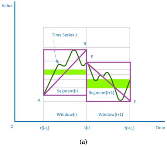
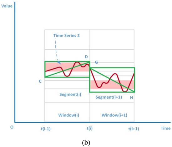
Figure 2. Summary of time series 1 and 2. (a) Summary of time series 1 (b) Summary of time series 2.

For the similarity of the subseries (i) of TimeSeries1 and TimeSeries2 in Figure 2, we may use the number of transformation steps of the segment AB and the segment CD to measure it. We call the number of transformation steps the transformation distance (TD), as shown in Figure 3. From CD to AB, this goes through vertical translation transformation (Figure 3a,b), rotation transformation (Figure 3b,c) and scale transformation (Figure 3c,d). The fewer transformation steps and the smaller the number of changes are, the higher the similarity is.

Figure 3. The transformations distance between AB and CD. (a) translation transformation; (b) rotation transformation; (c) scale transformation; (d) AB = CD.

Since the AB angle is arbitrary, it is not suitable for fast computing. The AB and the CD are transformed at the same time to make them parallel to the V axis, and then other transformations are performed to make them coincide, as shown in Figure 4.

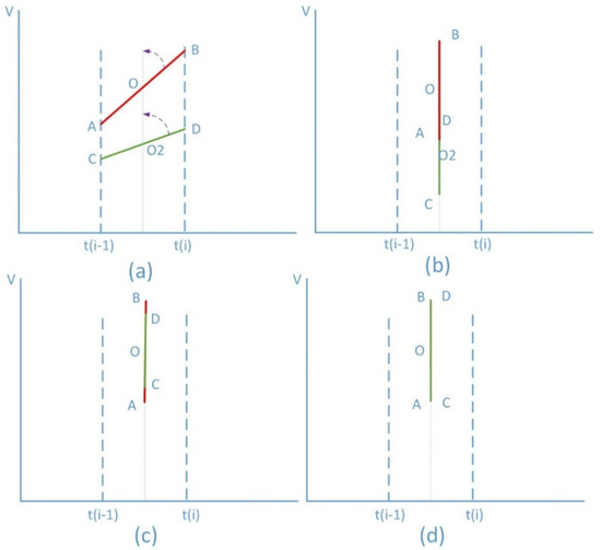
Figure 4. Change the order of the transformation distance calculation between AB and CD. (a) rotation transformation; (b) translation transformation; (c) scale transformation; (d) AB = CD.

After this transformation, AB and CD can be rotated by angles α and β, respectively, so that the summary segment is always parallel to the axis V and the value of point B is always greater than the value of point A (shown in Figure 5). We call the transformed segments AB and CD transformable interval objects (TIO). The two TIOs can be represented by the following Formula:

$$TI{O}_{AB}=(V_A,V_B,\alpha )$$

(2)

$$TI{O}_{CD}=(V_C,V_D,\beta )$$

(3)

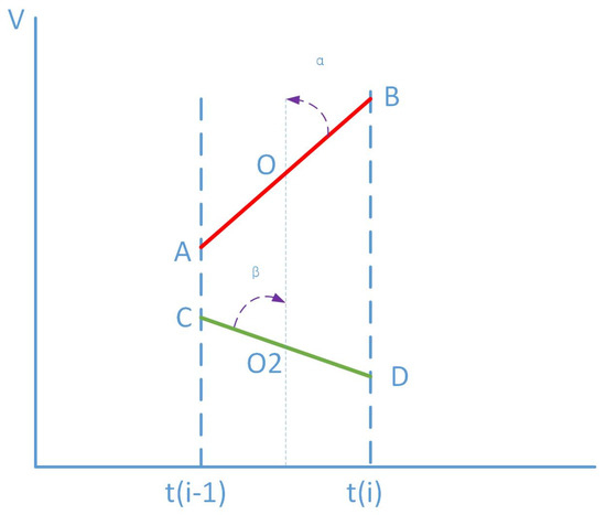
Figure 5. Transformable interval objects AB and CD.

Given that the distance between the center point of TIO_AB and the center point of TIO_CD is D₀, and S₀ is the scaling variable, the similarity distance between TIO_AB and TIO_CD is noted as:

$$DIST(TI{O}_{AB},TI{O}_{CD})=a\times \left|D_0\right|+b\times \left|\alpha -\beta \right|+c\times \left|S_0-1\right|$$

(4)

where D₀ is calculated by the Formula (5)

$$D_0=((V_A+V_B)-(V_C+V_D))∕2$$

(5)

and S₀ can be calculated by the Formula (6).

$$S_0=(V_B-V_A)\times cos\beta /(V_C-V_C)\times cos\alpha$$

(6)

The larger the DIST is, the smaller the similarity is, where a is the translation transformation factor, b is the angle transformation factor and c is the expansion transformation factor. Generally, the translation transformation factor and the rotation transformation angle factor have a greater effect, and the scaling transformation factor has a smaller effect. Therefore, Formula (4) can discard $c\times \left|S_0-1\right|$ while calculating the approximate similarity distance, and V_M can be the average value of the subseries. In Formula (5), D₀ can be approximated by the difference between the average value of the two subseries. In this way, each TIO can be expressed as Formula (7):

$$\mathrm{TIO}=(V_M,A)$$

(7)

where $V_M$ is the median value of V in Formulas (2) and (3), and A is still the angle to the axis V in the range (−90, 90).

Let V be the vertical coordinate axis and let angle A be the horizontal coordinate axis. A two-dimensional plane called the TIO plane has been constructed, and each TIO is a point on the plane, as illustrated in Figure 6, which shows the TIO points corresponding to the four subseries in Figure 2. On the two-dimensional TIO plane, the points with greater similarity are closer to each other in that space. Generally, the TIO plane can be divided into many areas, such as 64, 128, 256 or 512, etc. To save storage space, we can divide the plane into at least 16 and up to 256 areas. This allows each area to be represented by an 8 bits number. The higher the area count is, the more accurate the distance measure between two sequences is; however, the more the count of areas, the more difficult the computation as well. To map an area into a single digit, the TIO plane is divided into sixteen areas in this paper. Each area is represented by a hexadecimal number from 0 to F, as shown in Figure 7. Each TIO point must fall into one of the areas. The hexadecimal code of this area is used to represent the point. In that way, a subseries can be converted into a TIO point and finally to a hexadecimal digit. Therefore, a time series can be represented as a hexadecimal string. For example, Figure 2a can be represented by a hexadecimal string as “04”, and Figure 2b as “35”. This is also how we obtain the full name of HAX: the Hexadecimal Aggregate approXimation representation.

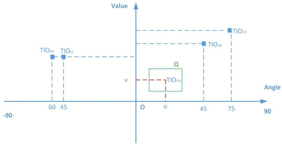
Figure 6. TIO points on the TIO plane.

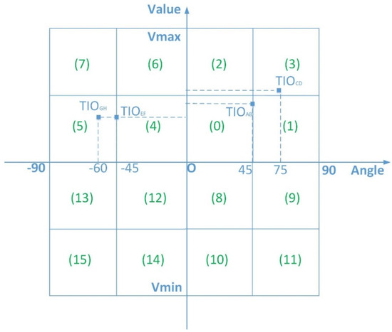
Figure 7. A 4 × 4 HAX grid plane.

3.2. HAX Distance Measures

The HAX transformation principle has been described in detail in the above section. Based on the principle, time-series objects can be easily converted into HAX strings, and the similarity between two time series objects can be measured by the distance between two corresponding HAX strings. This process can be described using the following Formula. Given a time series T which contains n values,

T = {v₁, v₂, …, v_n}

(8)

T is split into w segments S by PAA (paaMapper),

S = paaMapper(T) = {s₁,s₂, …,s_w}

(9)

where s_i is ith subseries. Via the TIO transformation, each subseries in S can be converted into a TIO point in a set of TIO points P,

P = tioMapper(S) = {p₁,p₂, …, p_w}

(10)

where p_j is a coordinate (s_j, a_j) and a_j is a rotation angle of segment(j) corresponding to subseries(j). Each point corresponds to a HAX character and P can then be converted into a HAX string H through the transformation haxMapper,

H = haxMapper(P) = {h₁,h₂, …, h_w}

(11)

Therefore, the approximate distance between two time series can be estimated by the distance between two corresponding HAX strings. Next, we discuss how to calculate the distance between two HAX characters.

Given two time series objects T^q and T^c, the similarity between these two can be estimated by many kinds of distances. The most commonly used is the Euclidean distance (ED), as follows:

$$\mathrm{ED}(T^q,T^c)=\sqrt[2]{{\displaystyle \sum }_{i=1}^n{(v_i^q-v_i^c)}^2}$$

(12)

However, the real time computation of ED is very inefficient for long time series. Hence the PAA splits a long time series into w short segments to reduce the dimension of the time series and adopt the segment distance (SD) to estimate the similarity as follows:

$$\mathrm{SD}(S^q,S^c)=\sqrt[2]{{\displaystyle \sum }_{j=1}^w{(s_j^q-s_j^c)}^2}$$

(13)

where

$$s_j=\frac{w}{n}{\displaystyle \sum }_{j=(n/w)(i+1)+1}^{(n/w)i}{v}_j$$

(14)

Although the SD decreases the computation of ED, it also discards the trend of a time series. Therefore, the PAX distance (PD) in this paper is expressed by TIO points and is designed to take into account the impact of the trend. The Formula is as follows:

$$\mathrm{PD}(P^q,P^c)=\sqrt[2]{{\displaystyle \sum }_{j=1}^w{(p_j^q-p_j^c)}^2}=\sqrt[2]{{\displaystyle \sum }_{j=1}^w({(s_j^q-s_j^c)}^2+f{(a_j^q-a_j^c)}^2)}$$

(15)

where f is a real number between (0, 1), used to adjust the weight between the V axis distance and the A axis (angle) distance so that the difference between PD and ED approaches 0 as much as possible. If there is no adjustment weight, f = 1. We call this method Point Aggregate approXimation representation (PAX).

The PAX enhances the accuracy of the similarity measurement of time series, but there are two factors in this method, and it is not convenient for character variables. Then, we use the haxMapper to map it to a hexadecimal character. The distance between the HAX (HD) strings H^q and H^c is used to measure the similarity distance between the two time series, denoted as

$$\begin{gathered} \mathrm{HD}(H^q,H^c)=\sqrt[2]{{\displaystyle \sum }_{j=1}^w{\left(haxMapper\left(p_j^q\right)-haxMapper(p_j^c\right))}^2} \\ =\sqrt[2]{{\displaystyle \sum }_{j=1}^w{\left(h_j^q-h_j^c\right)}^2} \end{gathered}$$

(16)

where haxMapper may have different mapping ways, using either sequential grid coding mapping or other mapping methods such as the Hilbert curve filling or Z-Ordering curve filling methods. This paper focuses on the basic sequential grid coding method, shown in Figure 7.

4. Experimental Evaluation

To verify the representation method proposed in this paper, we conducted an experimental evaluation for the HAX method and compared it with the SAX. The SAX method was selected because the SAX and the HAX methods are both symbol-based representation methods based on the PAA division and have the same string length for a time series object. In addition, the PAX method is a middle process result of the HAX and the length of its representation string is 16 times that of the HAX. Therefore, our experimental evaluation included the PAX and ED methods.

Since the analysis of time series data, which is based on the calculation of the similarity distance regardless of whether it is classification, clustering or query, we selected the simplest and most representative: the one nearest neighbor (1-NN) classification method [68] for the experiments of comparison [55,68,69]. All algorithms were implemented in Java, and the source code can be found at https://github.com/zhenwenhe/series.git, accessed on 29 September 2021. Next, we introduce the experimental data set and method parameter settings and then analyze the experimental results.

4.1. Experimental Data

This experiment used the latest time-series data set UCRArchive2018 [7]. The data set has been widely used in time series data analysis and mining algorithm experiments since 2002. After expansion in 2015 and 2018, UCRArchive2018 contains a total of 128 data sets. There are 14 data sets that are variable-length. Variable-length refers to the different lengths of sequences in the dataset and is not a very common time series. Since we did not consider the similarity measurement between variable-length time series data in the implementation of the algorithm, the experiment in this paper eliminated the 14 variable-length data sets. The data list used is shown in Table 3. The column ID is the order number of each data set in UCRArchive2018, which ranges from 1 to 144. The column Type shows the time series data type of each data set. The column Name is the name of each data set. The column Train is the number of series for the train set, and the column Test is the number of series for the test set. The column Class presents the class number in each data set in the UCRArchive2018. The column Length presents the point number of the correspondent time series in the data set. Each dataset has two parts, Train and Test, one for training the parameters and the other for the testing test. The datasets contain classes ranging from 2 to 60 and have the lengths of time series varying from 15 to 2844. The database was used in many recent papers [9,11]. We intend to cover time series in finance and economics in future works.

Table 3. A list of test data sets.

ID	Type	Name	Train	Test	Class	Length
1	Device	ACSF1	100	100	10	1460
2	Image	Adiac	390	391	37	176
3	Image	ArrowHead	36	175	3	251
4	Spectro	Beef	30	30	5	470
5	Image	BeetleFly	20	20	2	512
6	Image	BirdChicken	20	20	2	512
7	Simulated	BME	30	150	3	128
8	Sensor	Car	60	60	4	577
9	Simulated	CBF	30	900	3	128
10	Traffic	Chinatown	20	343	2	24
11	Sensor	ChlorineConcentration	467	3840	3	166
12	Sensor	CinCECGTorso	40	1380	4	1639
13	Spectro	Coffee	28	28	2	286
14	Device	Computers	250	250	2	720
15	Motion	CricketX	390	390	12	300
16	Motion	CricketY	390	390	12	300
17	Motion	CricketZ	390	390	12	300
18	Image	Crop	7200	16,800	24	46
19	Image	DiatomSizeReduction	16	306	4	345
20	Image	DistalPhalanxOutlineAgeGroup	400	139	3	80
21	Image	DistalPhalanxOutlineCorrect	600	276	2	80
22	Image	DistalPhalanxTW	400	139	6	80
23	Sensor	Earthquakes	322	139	2	512
24	ECG	ECG200	100	100	2	96
25	ECG	ECG5000	500	4500	5	140
26	ECG	ECGFiveDays	23	861	2	136
27	Device	ElectricDevices	8926	7711	7	96
28	EOG	EOGHorizontalSignal	362	362	12	1250
29	EOG	EOGVerticalSignal	362	362	12	1250
30	Spectro	EthanolLevel	504	500	4	1751
31	Image	FaceAll	560	1690	14	131
32	Image	FaceFour	24	88	4	350
33	Image	FacesUCR	200	2050	14	131
34	Image	FiftyWords	450	455	50	270
35	Image	Fish	175	175	7	463
36	Sensor	FordA	3601	1320	2	500
37	Sensor	FordB	3636	810	2	500
38	Sensor	FreezerRegularTrain	150	2850	2	301
39	Sensor	FreezerSmallTrain	28	2850	2	301
40	HRM	Fungi	18	186	18	201
41	Motion	GunPoint	50	150	2	150
42	Motion	GunPointAgeSpan	135	316	2	150
43	Motion	GunPointMaleVersusFemale	135	316	2	150
44	Motion	GunPointOldVersusYoung	136	315	2	150
45	Spectro	Ham	109	105	2	431
46	Image	HandOutlines	1000	370	2	2709
47	Motion	Haptics	155	308	5	1092
48	Image	Herring	64	64	2	512
49	Device	HouseTwenty	40	119	2	2000
50	Motion	InlineSkate	100	550	7	1882
51	EPG	InsectEPGRegularTrain	62	249	3	601
52	EPG	InsectEPGSmallTrain	17	249	3	601
53	Sensor	InsectWingbeatSound	220	1980	11	256
54	Sensor	ItalyPowerDemand	67	1029	2	24
55	Device	LargeKitchenAppliances	375	375	3	720
56	Sensor	Lightning2	60	61	2	637
57	Sensor	Lightning7	70	73	7	319
58	Simulated	Mallat	55	2345	8	1024
59	Spectro	Meat	60	60	3	448
60	Image	MedicalImages	381	760	10	99
61	Traffic	MelbournePedestrian	1194	2439	10	24
62	Image	MiddlePhalanxOutlineAgeGroup	400	154	3	80
63	Image	MiddlePhalanxOutlineCorrect	600	291	2	80
64	Image	MiddlePhalanxTW	399	154	6	80
65	Image	MixedShapesRegularTrain	500	2425	5	1024
66	Image	MixedShapesSmallTrain	100	2425	5	1024
67	Sensor	MoteStrain	20	1252	2	84
68	ECG	NonInvasiveFetalECGThorax1	1800	1965	42	750
69	ECG	NonInvasiveFetalECGThorax2	1800	1965	42	750
70	Spectro	OliveOil	30	30	4	570
71	Image	OSULeaf	200	242	6	427
72	Image	PhalangesOutlinesCorrect	1800	858	2	80
73	Sensor	Phoneme	214	1896	39	1024
74	Hemodynamics	PigAirwayPressure	104	208	52	2000
75	Hemodynamics	PigArtPressure	104	208	52	2000
76	Hemodynamics	PigCVP	104	208	52	2000
77	Sensor	Plane	105	105	7	144
78	Power	PowerCons	180	180	2	144
79	Image	ProximalPhalanxOutlineAgeGroup	400	205	3	80
80	Image	ProximalPhalanxOutlineCorrect	600	291	2	80
81	Image	ProximalPhalanxTW	400	205	6	80
82	Device	RefrigerationDevices	375	375	3	720
83	Spectrum	Rock	20	50	4	2844
84	Device	ScreenType	375	375	3	720
85	Spectrum	SemgHandGenderCh2	300	600	2	1500
86	Spectrum	SemgHandMovementCh2	450	450	6	1500
87	Spectrum	SemgHandSubjectCh2	450	450	5	1500
88	Simulated	ShapeletSim	20	180	2	500
89	Image	ShapesAll	600	600	60	512
90	Device	SmallKitchenAppliances	375	375	3	720
91	Simulated	SmoothSubspace	150	150	3	15
92	Sensor	SonyAIBORobotSurface1	20	601	2	70
93	Sensor	SonyAIBORobotSurface2	27	953	2	65
94	Sensor	StarLightCurves	1000	8236	3	1024
95	Spectro	Strawberry	613	370	2	235
96	Image	SwedishLeaf	500	625	15	128
97	Image	Symbols	25	995	6	398
98	Simulated	SyntheticControl	300	300	6	60
99	Motion	ToeSegmentation1	40	228	2	277
100	Motion	ToeSegmentation2	36	130	2	343
101	Sensor	Trace	100	100	4	275
102	ECG	TwoLeadECG	23	1139	2	82
103	Simulated	TwoPatterns	1000	4000	4	128
104	Simulated	UMD	36	144	3	150
105	Motion	UWaveGestureLibraryAll	896	3582	8	945
106	Motion	UWaveGestureLibraryX	896	3582	8	315
107	Motion	UWaveGestureLibraryY	896	3582	8	315
108	Motion	UWaveGestureLibraryZ	896	3582	8	315
109	Sensor	Wafer	1000	6164	2	152
110	Spectro	Wine	57	54	2	234
111	Image	WordSynonyms	267	638	25	270
112	Motion	Worms	181	77	5	900
113	Motion	WormsTwoClass	181	77	2	900
114	Image	Yoga	300	3000	2	426

4.2. Experimental Parameter Setting

Since both the HAX and the SAX methods are based on PAA division, the parameter w represents the dimension size in the PAA. In addition, the alpha parameter represents the alphabet size in the SAX. In our experiment, the two methods used the same w parameter. For each data set, the range of w was [5,20]. For the SAX method and each w, the range of the corresponding parameter alpha was [3,16]. According to the existing references about SAX, the nearest neighbor classification accuracy results for SAX are always the best for the UCRArchive2018 when the range of w is [5,20] and the range of the corresponding parameter alpha is [3,16]. The score is computed for each w for HAX and each combination of w and alpha for the SAX method. Therefore, we used the average score to measure the accuracy. The classification algorithm 1-NN was used to classify each different parameter setting of each data set, and then a calculation of the classification accuracy scores was carried out. For example, for each data set in the experimental database, the HAX method would calculate 16 scores and then get an average value of the scores; while the SAX method would calculate 16 × 14 scores and then compute the average score. We used the average of this classification accuracy rate as a measured variable.

4.3. Experimental Results and Analysis

Four methods, the SAX, SAX_TD, SAX-BD and ED, were the baseline methods, and the classification accuracy of each representation method was calculated based on the 1-NN. Table 4 shows the experimental results. The column ID is the identifier of the data set in Table 3. The columns, ED, PAX, HAX, SAX, SAX-TD and SAX-BD, are the representation methods’ names. The values in each column of the methods are the classification accuracy values. Figure 8 shows the results in a plot. Our previous work [62] presented the comparison results among SAX, ESAX, SAX-TD and SAX-BD. Here we will focus on the comparison of HAX, SAX, PAX, SAX-BD and ED.

Table 4. Classification accuracy on UCRArchive2018.

ID	ED	SAX	SAX-TD	SAX-BD	PAX	HAX
1	0.54	0.13	0.63	0.60	0.38	0.23
2	0.61	0.08	0.59	0.74	0.47	0.15
3	0.80	0.52	0.75	0.84	0.73	0.56
4	0.83	0.70	0.81	0.80	0.84	0.88
5	0.67	0.40	0.58	0.90	0.60	0.51
6	0.75	0.72	0.75	0.80	0.74	0.75
7	0.55	0.57	0.59	0.94	0.63	0.58
8	0.85	0.84	0.88	0.88	0.96	0.71
9	0.73	0.49	0.70	0.97	0.67	0.53
10	0.95	0.76	0.93	0.96	0.81	0.70
11	0.65	0.42	0.54	0.94	0.58	0.46
12	0.90	0.66	0.75	1.00	0.79	0.71
13	1.00	0.51	0.95	0.62	0.90	0.62
14	0.58	0.51	0.53	0.67	0.52	0.57
15	0.58	0.43	0.55	0.63	0.59	0.27
16	0.57	0.43	0.52	0.68	0.61	0.26
17	0.59	0.44	0.56	0.97	0.62	0.33
18	0.71	0.28	0.68	0.73	0.70	0.34
19	0.93	0.24	0.95	0.75	0.91	0.67
20	0.63	0.53	0.66	0.63	0.68	0.62
21	0.72	0.57	0.71	0.71	0.71	0.63
22	0.63	0.42	0.58	0.91	0.60	0.54
23	0.88	0.80	0.88	0.88	0.87	0.80
24	0.92	0.87	0.92	0.40	0.92	0.89
25	0.80	0.68	0.82	0.40	0.80	0.68
26	0.42	0.29	0.36	0.30	0.41	0.21
27	0.44	0.30	0.40	0.79	0.34	0.23
28	0.71	0.66	0.68	0.88	0.65	0.66
29	0.55	0.43	0.57	0.83	0.58	0.48
30	0.27	0.25	0.28	0.68	0.28	0.27
31	0.71	0.35	0.72	0.83	0.69	0.35
32	0.78	0.53	0.72	0.69	0.80	0.69
33	0.77	0.40	0.65	0.61	0.74	0.39
34	0.63	0.54	0.63	0.86	0.66	0.49
35	0.78	0.25	0.70	0.96	0.68	0.24
36	0.67	0.51	0.57	0.94	0.57	0.53
37	0.61	0.51	0.52	0.99	0.52	0.51
38	0.80	0.66	0.88	1.00	0.91	0.63
39	0.68	0.67	0.69	0.68	0.70	0.67
40	0.82	0.54	0.80	0.88	0.88	0.46
41	0.91	0.72	0.87	0.43	0.92	0.75
42	0.90	0.65	0.91	0.63	0.98	0.83
43	0.97	0.65	0.99	0.80	0.99	0.87
44	0.95	0.64	1.00	0.35	1.00	1.00
45	0.60	0.54	0.59	0.78	0.58	0.58
46	0.86	0.62	0.85	0.68	0.82	0.75
47	0.37	0.29	0.35	0.58	0.35	0.31
48	0.52	0.52	0.53	0.95	0.54	0.53
49	0.66	0.67	0.69	0.58	0.64	0.61
50	0.34	0.25	0.29	0.85	0.33	0.25
51	0.68	0.41	0.67	0.73	1.00	1.00
52	0.66	0.20	0.59	0.93	1.00	1.00
53	0.56	0.43	0.53	0.68	0.54	0.45
54	0.96	0.82	0.95	0.91	0.95	0.89
55	0.49	0.42	0.49	0.53	0.53	0.38
56	0.75	0.69	0.74	0.74	0.78	0.60
57	0.58	0.50	0.56	0.52	0.66	0.37
58	0.91	0.39	0.83	0.88	0.90	0.54
59	0.93	0.33	0.91	0.82	0.91	0.46
60	0.68	0.51	0.67	0.88	0.69	0.48
61	0.85	0.43	0.92	0.90	0.82	0.41
62	0.52	0.36	0.49	0.56	0.50	0.42
63	0.77	0.53	0.72	0.77	0.73	0.61
64	0.51	0.29	0.51	0.12	0.53	0.41
65	0.90	0.79	0.86	0.18	0.87	0.76
66	0.84	0.74	0.80	0.35	0.81	0.71
67	0.88	0.75	0.82	0.14	0.84	0.75
68	0.83	0.13	0.72	1.00	0.73	0.17
69	0.88	0.15	0.80	0.97	0.77	0.20
70	0.52	0.45	0.50	0.82	0.50	0.40
71	0.87	0.30	0.85	0.87	0.81	0.31
72	0.76	0.56	0.72	0.76	0.72	0.62
73	0.11	0.06	0.07	0.48	0.09	0.06
74	0.06	0.05	0.08	0.86	0.12	0.06
75	0.13	0.02	0.11	0.45	0.22	0.11
76	0.08	0.04	0.05	0.95	0.14	0.06
77	0.96	0.73	0.96	0.79	0.96	0.87
78	0.93	0.81	0.91	0.88	0.97	0.87
79	0.79	0.48	0.78	0.64	0.77	0.64
80	0.81	0.57	0.76	0.77	0.74	0.64
81	0.71	0.36	0.70	0.64	0.70	0.58
82	0.39	0.36	0.38	0.94	0.39	0.35
83	0.84	0.46	0.72	0.76	0.54	0.68
84	0.36	0.38	0.37	0.86	0.39	0.37
85	0.76	0.55	0.63	0.96	0.80	0.56
86	0.37	0.25	0.33	0.88	0.60	0.22
87	0.40	0.33	0.37	0.91	0.70	0.31
88	0.54	0.50	0.50	0.95	0.49	0.50
89	0.75	0.53	0.71	0.75	0.72	0.53
90	0.34	0.44	0.58	0.88	0.58	0.53
91	0.91	0.52	0.84	1.00	0.97	0.85
92	0.70	0.64	0.66	0.94	0.74	0.64
93	0.86	0.78	0.84	0.95	0.84	0.79
94	0.85	0.80	0.87	0.99	0.88	0.84
95	0.95	0.57	0.93	1.00	0.92	0.76
96	0.79	0.38	0.74	0.57	0.76	0.37
97	0.90	0.76	0.88	0.62	0.89	0.81
98	0.88	0.87	0.89	0.56	0.98	0.66
99	0.68	0.63	0.64	0.69	0.68	0.60
100	0.81	0.81	0.83	0.83	0.85	0.74
101	0.76	0.49	0.66	0.86	0.76	0.59
102	0.75	0.59	0.77	0.73	0.70	0.65
103	0.91	0.78	0.88	0.83	0.91	0.51
104	0.76	0.64	0.77	0.79	0.78	0.68
105	0.95	0.81	0.92	0.88	0.92	0.72
106	0.74	0.66	0.72	0.71	0.73	0.61
107	0.66	0.58	0.65	0.65	0.67	0.51
108	0.65	0.59	0.64	0.65	0.65	0.55
109	1.00	0.98	0.99	0.99	0.99	0.98
110	0.61	0.50	0.55	0.55	0.61	0.51
111	0.62	0.51	0.59	0.61	0.63	0.47
112	0.45	0.47	0.50	0.5	0.52	0.40
113	0.61	0.59	0.60	0.61	0.62	0.54
114	0.83	0.67	0.80	0.78	0.81	0.69

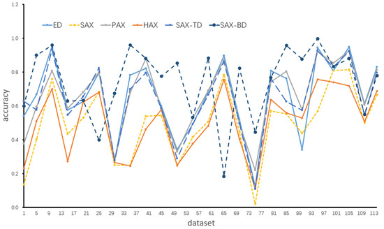
Figure 8. Accuracy comparison plot for Table 4.

The results in Table 4 show that the classification accuracy of the PAX is significantly higher than those of the HAX and SAX methods, and the HAX has some advantages over the SAX classification accuracy. Figure 9 makes the comparison between the HAX and SAX methods more obvious. The X-axis value is the accuracy of the SAX, the Y-axis value is the accuracy of the HAX and the scattered points are mostly in the upper triangle (71 points in the upper triangle and 43 points in the lower triangle). This shows that the accuracy of the HAX is larger than the SAX. Figure 10 makes the comparison between the PAX and SAX methods more obvious. Almost all the scattered points in Figure 10 are in the upper triangle, which shows that the accuracy of the PAX is significantly larger than the SAX.

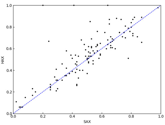
Figure 9. Accuracy comparison between HAX and SAX (71 points in the upper triangle and 43 points in the lower triangle).

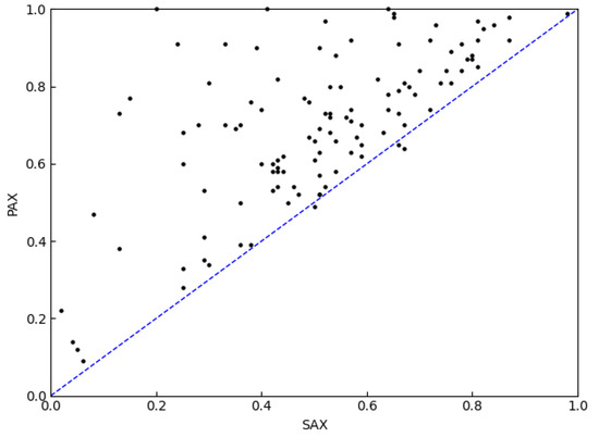
Figure 10. Accuracy comparison between PAX and SAX (111 points in the upper triangle and 3 points in the lower triangle).

The ED is still widely used in equal length time series measurements. In our work, we selected the ED and SAX methods as baselines. Figure 11 shows the accuracy comparison among the HAX, the ED and the SAX. The results show that ED still has higher accuracy when compared with the SAX and HAX methods. Figure 12 shows the accuracy comparison among the PAX, the ED and the SAX. It shows that the accuracy rates of the PAX and ED are very close. Figure 13 makes the comparison between the PAX and ED methods more obvious. About half of the scattered points in Figure 13 are in the upper triangle. Figure 14 makes the comparison between the PAX and SAX-BD methods more obvious. These figures show that the accuracy of PAX is lower than the ED and SAX-BD methods but very close to them.

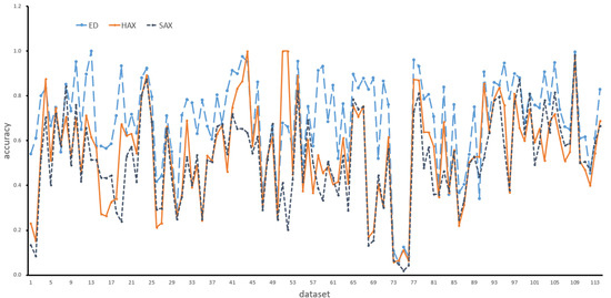
Figure 11. Accuracy comparison among HAX, ED and SAX.

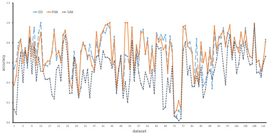
Figure 12. Accuracy comparison among PAX, ED and SAX.

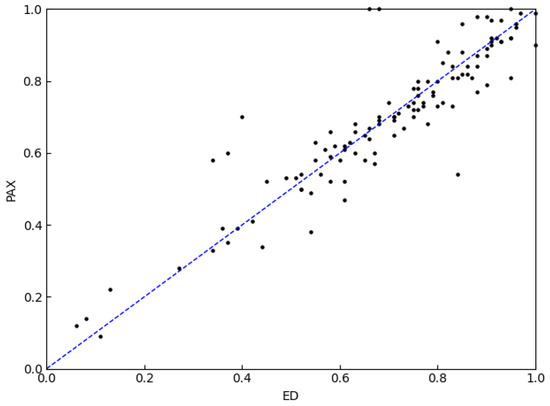
Figure 13. Accuracy comparison between PAX and ED (48 points in the upper triangle and 63 points in the lower triangle).

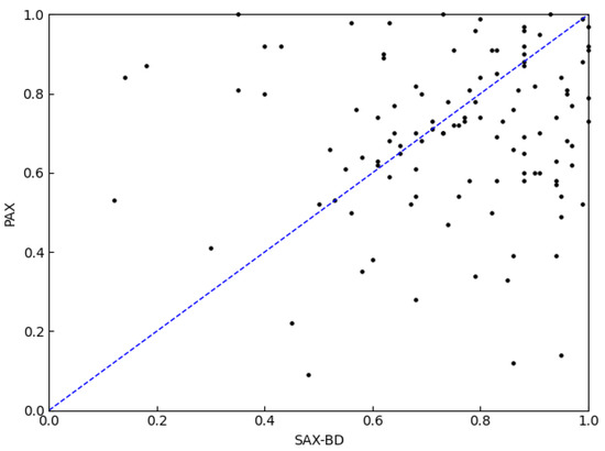
Figure 14. Accuracy comparison between PAX and SAX-BD (50 points in the upper triangle and 54 points in the lower triangle).

In terms of space cost, the HAX realizes the dimensionality reduction of high-dimensional time series by representing a time series as a set of hex strings, reducing the amount of information required for time series storage and making it more convenient to be used in various fields. For a time series with the same parameter w, the length of the hex string is equal to that of the SAX string. While the space cost of SAX-TD is five times that of the SAX, the space cost of SAX-BD is nine times that of the SAX. Although the PAX has higher accuracy than the HAX, it only implements the reduction of the time series to a set two-dimensional data point, and the space cost of PAX is sixteen times greater than that of the HAX. Therefore, they have the following relationship,

$$\mathrm{SC}(\mathrm{HAX})=\mathrm{SC}(\mathrm{SAX})=\mathrm{SC}(\mathrm{SAX}-\mathrm{TD})/5=\mathrm{SC}(\mathrm{SAX}-\mathrm{BD})/9=\mathrm{SC}(\mathrm{PAX})/16=\frac{w}{n}\mathrm{SC}(\mathrm{ED})$$

(17)

in which the SC is a space cost function, n is the length of a time series and w is the piece parameter.

5. Conclusions

In this paper, two new time series representation methods, the Hexadecimal Aggregation approXimate (HAX) and the Point Aggregation approXimate (PAX), are proposed. These two methods negate any assumption on the probability distribution of time series and initially represent each segment of a time series as a Transformable Interval Object (TIO). Then, each TIO is mapped to a spatial point located on a two-dimensional plane. The PAX represents each segment of a time series as a spatial point on the plane. Next, the HAX maps each point of the PAX to a hexadecimal digit by a hexagon grid. Finally, a hex string that can represent a time series is generated by the HAX. The experiment results show that the HAX has higher classification accuracy than the SAX, but one that is lower than most SAX variants, such as SAX-TD and SAX-BD. This is because these variants include some other information that may improve the distance measure of the SAX string. The HAX has the same space cost as the SAX and a lower space cost than the above-mentioned SAX variants. The PAX has higher classification accuracy than the HAX and is very close to the ED, but its space cost is 16 times that of the HAX. However, the space cost of the PAX is generally much less than the space cost of the ED. The HAX is a general time series representation method that can be extended similar to some SAX variants. Our future work will focus on the extension of HAX.

References

- He, Z.; Kraak, M.-J.; Huisman, O.; Ma, X.; Xiao, J. Parallel indexing technique for spatio-temporal data. ISPRS J. Photogramm. Remote. Sens. 2013, 78, 116–128. [Google Scholar] [CrossRef]
- He, Z.; Wu, C.; Liu, G.; Zheng, Z.; Tian, Y. Decomposition tree: A spatio-temporal indexing method for movement big data. Clust. Comput. 2015, 18, 1481–1492. [Google Scholar] [CrossRef]
- He, Z.; Ma, X. A distributed indexing method for timeline similarity query. Algorithms 2018, 11, 41. [Google Scholar] [CrossRef] [Green Version]
- Hamilton, J.D. Time Series Analysis; Princeton University Press: Princeton, NJ, USA, 2020. [Google Scholar]
- Chatfield, C.; Xing, H. The Analysis of Time Series: An Introduction with R; Chapman and Hall/CRC: Boca Raton, FL, USA, 2019. [Google Scholar]
- Hyndman, R.J.; Athanasopoulos, G. Forecasting: Principles and Practice; OTexts: Melbourne, Australia, 2018. [Google Scholar]
- Dau, H.A.; Bagnall, A.; Kamgar, K.; Yeh, C.-C.M.; Zhu, Y.; Gharghabi, S.; Ratanamahatana, C.A.; Keogh, E. The UCR time series archive. IEEE/CAA J. Autom. Sin. 2019, 6, 1293–1305. [Google Scholar] [CrossRef]
- Kondylakis, H.; Dayan, N.; Zoumpatianos, K.; Palpanas, T. Coconut: A scalable bottom-up approach for building data series indexes. arXiv Prepr. 2020, arXiv:2006.13713. [Google Scholar]
- Oregi, I.; Pérez, A.; Del Ser, J.; Lozano, J.A. On-line elastic similarity measures for time series. Pattern Recognit. 2019, 88, 506–517. [Google Scholar] [CrossRef]
- Aghabozorgi, S.; Seyed Shirkhorshidi, A.; Ying Wah, T. Time-series clustering–A decade review. Inf. Syst. 2015, 53, 16–38. [Google Scholar] [CrossRef]
- Ismail Fawaz, H.; Forestier, G.; Weber, J.; Idoumghar, L.; Muller, P.-A. Deep learning for time series classification: A review. Data Min. Knowl. Discov. 2019, 33, 917–963. [Google Scholar] [CrossRef] [Green Version]
- Chan, K.-P.; Fu, A.W.-C. Efficient time series matching by wavelets. In Proceedings of the 15th International Conference on Data Engineering (Cat. No. 99CB36337), Sydney, Australia, 23–26 March 1999; pp. 126–133. [Google Scholar]
- Faloutsos, C.; Ranganathan, M.; Manolopoulos, Y.J.A.S.R. Fast subsequence matching in time-series databases. ACM Sigmod Rec. 1994, 23, 419–429. [Google Scholar] [CrossRef] [Green Version]
- Huang, Y.-W.; Yu, P.S. Adaptive query processing for time-series data. In Proceedings of the Fifth ACM SIGKDD International Conference on Knowledge Discovery and Data Mining, San Diego, CA, USA, 15–18 August 1999; pp. 282–286. [Google Scholar]
- Geurts, P. Pattern extraction for time series classification. In Proceedings of the European Conference on Principles of Data Mining and Knowledge Discovery, Freiburg, Germany, 3–5 September 2001; pp. 115–127. [Google Scholar]
- Chakrabarti, K.; Keogh, E.; Mehrotra, S.; Pazzani, M. Locally adaptive dimensionality reduction for indexing large time series databases. ACM Trans. Database Syst. 2002, 27, 188–228. [Google Scholar] [CrossRef]
- Keogh, E.J.; Pazzani, M.J. An enhanced representation of time series which allows fast and accurate classification, clustering and relevance feedback. In Proceedings of the Knowledge Discovery in Databases, New York, NY, USA, 27–31 August 1998; pp. 239–243. [Google Scholar]
- Keogh, E.; Chakrabarti, K.; Pazzani, M.; Mehrotra, S. Dimensionality reduction for fast similarity search in large time series databases. Inf. Syst. 2001, 3, 263–286. [Google Scholar] [CrossRef]
- Lin, J.; Keogh, E.; Lonardi, S.; Chiu, B. A symbolic representation of time series, with implications for streaming algorithms. In Proceedings of the 8th ACM SIGMOD Workshop on Research Issues in Data Mining and Knowledge Discovery, San Diego, CA, USA, 13 June 2003; pp. 2–11. [Google Scholar]
- Chen, L.; Ng, R. On the marriage of lp-norms and edit distance. In Proceedings of the Thirtieth International Conference on Very Large Data Bases-Volume 30, Toronto, ON, Canada, 31 August–3 September 2004; pp. 792–803. [Google Scholar]
- Chairunnanda, P.; Gopalkrishnan, V.; Chen, L. Enhancing edit distance on real sequences filters using histogram distance on fixed reference ordering. In Proceedings of the 18th International Conference on Pattern Recognition (ICPR’06), Hong Kong, China, 20–24 August 2006; pp. 582–585. [Google Scholar]
- Lin, J.; Keogh, E.; Wei, L.; Lonardi, S. Experiencing SAX: A novel symbolic representation of time series. Data Min. Knowl. Discov. 2007, 15, 107–144. [Google Scholar] [CrossRef] [Green Version]
- Shieh, J.; Keogh, E. iSAX: Disk-aware mining and indexing of massive time series datasets. Data Min. Knowl. Discov. 2009, 19, 24–57. [Google Scholar] [CrossRef] [Green Version]
- Ye, L.; Keogh, E. Time series shapelets: A new primitive for data mining. In Proceedings of the 15th ACM SIGKDD International Conference on Knowledge Discovery and Data Mining, Paris, France, 28 June–1 July 2009; pp. 947–956. [Google Scholar]
- Camerra, A.; Palpanas, T.; Shieh, J.; Keogh, E. iSAX 2.0: Indexing and mining one billion time series. In Proceedings of the 2010 IEEE International Conference on Data Mining, Washington, DC, USA, 13–17 December 2010; pp. 58–67. [Google Scholar]
- He, X.; Shao, C.; Xiong, Y. A new similarity measure based on shape information for invariant with multiple distortions. Neurocomputing 2014, 129, 556–569. [Google Scholar] [CrossRef]
- Bai, S.; Qi, H.-D.; Xiu, N. Constrained best Euclidean distance embedding on a sphere: A matrix optimization approach. SIAM J. Optim. 2015, 25, 439–467. [Google Scholar] [CrossRef] [Green Version]
- Hsu, C.-J.; Huang, K.-S.; Yang, C.-B.; Guo, Y.-P. Flexible dynamic time warping for time series classification. Procedia Comput. Sci. 2015, 51, 2838–2842. [Google Scholar] [CrossRef] [Green Version]
- Roggen, D.; Cuspinera, L.P.; Pombo, G.; Ali, F.; Nguyen-Dinh, L.-V. Limited-memory warping LCSS for real-time low-power pattern recognition in wireless nodes. In Proceedings of the European Conference on Wireless Sensor Networks, Porto, Portugal, 9–11 February 2015; pp. 151–167. [Google Scholar]
- Ares, J.; Lara, J.A.; Lizcano, D.; Suárez, S. A soft computing framework for classifying time series based on fuzzy sets of events. Inf. Sci. 2016, 330, 125–144. [Google Scholar] [CrossRef]
- Zoumpatianos, K.; Idreos, S.; Palpanas, T. ADS: The adaptive data series index. Very Large Data Bases J. 2016, 25, 843–866. [Google Scholar] [CrossRef]
- Yagoubi, D.E.; Akbarinia, R.; Masseglia, F.; Palpanas, T. Dpisax: Massively distributed partitioned isax. In Proceedings of the 2017 IEEE International Conference on Data Mining (ICDM), New Orleans, LA, USA, 18–21 November 2017; pp. 1135–1140. [Google Scholar]
- Yagoubi, D.E.; Akbarinia, R.; Masseglia, F.; Shasha, D. RadiusSketch: Massively distributed indexing of time series. In Proceedings of the 2017 IEEE International Conference on Data Science and Advanced Analytics (DSAA), Tokyo, Japan, 19–21 October 2017; pp. 262–271. [Google Scholar]
- Baldán, F.J.; Benítez, J.M. Distributed FastShapelet Transform: A Big Data time series classification algorithm. Inf. Sci. 2019, 496, 451–463. [Google Scholar] [CrossRef]
- Yagoubi, D.; Akbarinia, R.; Masseglia, F.; Palpanas, T. Massively distributed time series indexing and querying. IEEE Trans. Knowl. Data Eng. 2020, 32, 108–120. [Google Scholar] [CrossRef] [Green Version]
- Serra, J.; Kantz, H.; Serra, X.; Andrzejak, R.G. Predictability of music descriptor time series and its application to cover song detection. IEEE Trans. Audio Speech Lang. Process. 2011, 20, 514–525. [Google Scholar] [CrossRef] [Green Version]
- Box, G.E.P.; Jenkins, G.M.; Reinsel, G.C.; Ljung, G.M. Time Series Analysis: Forecasting and Control; John Wiley & Sons: Hoboken, NJ, USA, 2015. [Google Scholar]
- Agrawal, R.; Faloutsos, C.; Swami, A. Efficient similarity search in sequence databases. In Proceedings of the Foundations of Data Organization and Algorithms, Berlin/Heidelberg, Germany, 21–23 June 1993; pp. 69–84. [Google Scholar]
- Kawagoe, K.; Ueda, T. A similarity search method of time series data with combination of Fourier and wavelet transforms. In Proceedings of the Ninth International Symposium on Temporal Representation and Reasoning, Manchester, UK, 7–9 July 2002; pp. 86–92. [Google Scholar]
- Korn, F.; Jagadish, H.V.; Faloutsos, C. Efficiently supporting ad hoc queries in large datasets of time sequences. ACM Sigmod Rec. 1997, 26, 289–300. [Google Scholar] [CrossRef]
- Azzouzi, M.; Nabney, I.T. Analysing time series structure with hidden Markov models. In Proceedings of the Neural Networks for Signal Processing VIII. Proceedings of the 1998 IEEE Signal Processing Society Workshop (Cat. No. 98TH8378), Cambridge, UK, 2 September 1998; pp. 402–408. [Google Scholar]
- Yi, B.-K.; Faloutsos, C. Fast time sequence indexing for arbitrary Lp norms. In Proceedings of the Very Large Data Bases, Cairo, Egypt, 10–14 September 2000. [Google Scholar]
- Keogh, E.J.; Pazzani, M.J. A simple dimensionality reduction technique for fast similarity search in large time series databases. In Proceedings of the Pacific-Asia Conference on Knowledge Discovery and Data Mining, Kyoto, Japan, 18–20 April 2000; pp. 122–133. [Google Scholar]
- Chung, F.L.K.; Fu, T.-C.; Luk, W.P.R.; Ng, V.T.Y. Flexible time series pattern matching based on perceptually important points. In Proceedings of the Workshop on Learning from Temporal and Spatial Data in International Joint Conference on Artificial Intelligence, Washington, DC, USA, 4–10 August 2001. [Google Scholar]
- Cai, Y.; Ng, R. Indexing spatio-temporal trajectories with Chebyshev polynomials. In Proceedings of the 2004 ACM SIGMOD International Conference on Management of Data, Paris France, 13–18 June 2004; pp. 599–610. [Google Scholar]
- Keogh, E.; Lin, J.; Fu, A. Hot SAX: Efficiently finding the most unusual time series subsequence. In Proceedings of the Fifth IEEE International Conference on Data Mining (ICDM’05), Washington, DC, USA, 27–30 November 2005; p. 8. [Google Scholar]
- Ratanamahatana, C.; Keogh, E.; Bagnall, A.J.; Lonardi, S. A novel bit level time series representation with implication of similarity search and clustering. In Proceedings of the Pacific-Asia Conference on Knowledge Discovery and Data Mining, Hanoi Vietnam, 18–20 May 2005; pp. 771–777. [Google Scholar]
- Lin, J.; Keogh, E. Group SAX: Extending the notion of contrast sets to time series and multimedia data. In Proceedings of the European Conference on Principles of Data Mining and Knowledge Discovery, Berlin, Germany, 18–22 September 2006; pp. 284–296. [Google Scholar]
- Lkhagva, B.; Suzuki, Y.; Kawagoe, K. Extended SAX: Extension of symbolic aggregate approximation for financial time series data representation. DEWS2006 4A-i8 2006, 7. Available online: https://www.ieice.org/~de/DEWS/DEWS2006/doc/4A-i8.pdf (accessed on 29 September 2021).
- Hung, N.Q.V.; Anh, D.T. Combining SAX and piecewise linear approximation to improve similarity search on financial time series. In Proceedings of the 2007 International Symposium on Information Technology Convergence (ISITC’2007), Washington, DC, USA, 23–24 November 2007; pp. 58–62. [Google Scholar]
- Chen, Q.; Chen, L.; Lian, X.; Liu, Y.; Yu, J.X. Indexable PLA for efficient similarity search. In Proceedings of the 33rd International Conference on Very Large Data Bases, Vienna Austria, 23–27 September 2007; pp. 435–446. [Google Scholar]
- Malinowski, S.; Guyet, T.; Quiniou, R.; Tavenard, R. 1d-SAX: A novel symbolic representation for time series. In Proceedings of the International Symposium on Intelligent Data Analysis, London UK, 17–19 October 2013; pp. 273–284. [Google Scholar]
- Stefan, A.; Athitsos, V.; Das, G. The move-split-merge metric for time series. IEEE Trans. Knowl. Data Eng. 2013, 25, 1425–1438. [Google Scholar] [CrossRef] [Green Version]
- Senin, P.; Malinchik, S. SAX-VSM: Interpretable time series classification using SAX and vector space model. In Proceedings of the 2013 IEEE 13th International Conference on Data Mining, Dallas, TX, USA, 7–10 December 2013; pp. 1175–1180. [Google Scholar]
- Kamath, U.; Lin, J.; Jong, K.D. SAX-EFG: An evolutionary feature generation framework for time series classification. In Proceedings of the 2014 Annual Conference on Genetic and Evolutionary Computation, Vancouver, BC, Canada, 12–16 July 2014; pp. 533–540. [Google Scholar]
- Baydogan, M.G.; Runger, G. Learning a symbolic representation for multivariate time series classification. Data Min. Knowl. Discov. 2014, 29, 400–422. [Google Scholar] [CrossRef]
- Zhang, Z.; Tang, P.; Duan, R. Dynamic time warping under pointwise shape context. Inf. Sci. 2015, 315, 88–101. [Google Scholar] [CrossRef]
- Baydogan, M.G.; Runger, G. Time series representation and similarity based on local autopatterns. Data Min. Knowl. Discov. 2015, 30, 476–509. [Google Scholar] [CrossRef]
- Ye, Y.; Jiang, J.; Ge, B.; Dou, Y.; Yang, K. Similarity measures for time series data classification using grid representation and matrix distance. Knowl. Inf. Syst. 2018, 60, 1105–1134. [Google Scholar] [CrossRef]
- Ruta, N.; Sawada, N.; McKeough, K.; Behrisch, M.; Beyer, J. SAX navigator: Time series exploration through hierarchical clustering. In Proceedings of the 2019 IEEE Visualization Conference (VIS), Vancouver, BC, Canada, 20–25 October 2019; pp. 236–240. [Google Scholar]
- Park, H.; Jung, J.-Y. SAX-ARM: Deviant event pattern discovery from multivariate time series using symbolic aggregate approximation and association rule mining. Expert Syst. Appl. 2020, 141, 112950. [Google Scholar] [CrossRef]
- He, Z.; Long, S.; Ma, X.; Zhao, H. A boundary distance-based symbolic aggregate approximation method for time series data. Algorithms 2020, 13, 284. [Google Scholar] [CrossRef]
- Bountrogiannis, K.; Tzagkarakis, G.; Tsakalides, P. Data-driven kernel-based probabilistic SAX for time series dimensionality reduction. In Proceedings of the 2020 28th European Signal Processing Conference (EUSIPCO), Amsterdam, The Netherlands, 24–28 August 2021; pp. 2343–2347. [Google Scholar]
- Sant’Anna, A.; Wickstrom, N. Symbolization of time-series: An evaluation of SAX, Persist, and ACA. In Proceedings of the 4th International Congress on Image and Signal Processing, CISP 2011, October 15, Shanghai, China, 15–17 October 2011; pp. 2223–2228. [Google Scholar]
- Camerra, A.; Shieh, J.; Palpanas, T.; Rakthanmanon, T.; Keogh, E. Beyond one billion time series: Indexing and mining very large time series collections with iSAX2+. Knowl. Inf. Syst. 2013, 39, 123–151. [Google Scholar] [CrossRef]
- Sun, Y.; Li, J.; Liu, J.; Sun, B.; Chow, C. An improvement of symbolic aggregate approximation distance measure for time series. Neurocomputing 2014, 138, 189–198. [Google Scholar] [CrossRef]
- Lkhagva, B.; Yu, S.; Kawagoe, K. New time series data representation ESAX for financial applications. In Proceedings of the 22nd International Conference on Data Engineering Workshops (ICDEW’06), Atlanta, GA, USA, 3–7 April 2006; p. x115. [Google Scholar]
- Altman, N.S. An introduction to kernel and nearest-neighbor nonparametric regression. Am. Stat. 1992, 46, 175–185. [Google Scholar]
- Abanda, A.; Mori, U.; Lozano, J.A. A review on distance based time series classification. Data Min. Knowl. Discov. 2019, 33, 378–412. [Google Scholar] [CrossRef] [Green Version]
Publisher’s Note: MDPI stays neutral with regard to jurisdictional claims in published maps and institutional affiliations. |
© 2021 by the authors. Licensee MDPI, Basel, Switzerland. This article is an open access article distributed under the terms and conditions of the Creative Commons Attribution (CC BY) license (https://creativecommons.org/licenses/by/4.0/).