A Sequential Graph Neural Network for Short Text Classification

Abstract

Short text classification is an important problem of natural language processing (NLP), and graph neural networks (GNNs) have been successfully used to solve different NLP problems. However, few studies employ GNN for short text classification, and most of the existing graph-based models ignore sequential information (e.g., word orders) in each document. In this work, we propose an improved sequence-based feature propagation scheme, which fully uses word representation and document-level word interaction and overcomes the limitations of textual features in short texts. On this basis, we utilize this propagation scheme to construct a lightweight model, sequential GNN (SGNN), and its extended model, ESGNN. Specifically, we build individual graphs for each document in the short text corpus based on word co-occurrence and use a bidirectional long short-term memory network (Bi-LSTM) to extract the sequential features of each document; therefore, word nodes in the document graph retain contextual information. Furthermore, two different simplified graph convolutional networks (GCNs) are used to learn word representations based on their local structures. Finally, word nodes combined with sequential information and local information are incorporated as the document representation. Extensive experiments on seven benchmark datasets demonstrate the effectiveness of our method.

1. Introduction

With the rapid development of network information technology, a large amount of short text data, such as book/movie reviews, online news, and product introductions, are increasingly generated on the Internet [1,2,3]. The existence of such unstructured data provides huge resources for data processing and management to mine useful information [4]. Automatic classification of these short text data is one of the most important tasks in NLP and it is a key prerequisite for the development of applications in different domains, such as news categorization, sentiment analysis, question-answer systems, dialogue systems, and query intent classification [5,6,7,8].

Traditional machine learning methods have initially been leveraged to solve the problem of short text classification [9]. Compared with long texts, short texts have fewer words and less descriptive information, which are sparse [10]. However, text representation obtained by feature engineering in this method is high-dimensional and highly sparse, each word is independent, ignoring the contextual relationship in the text, and the feature expression ability is very weak [11,12,13], which has a great impact on the accuracy of short text classification. Traditional machine learning methods cannot meet the needs of short text classification.

To obtain better features of textual data, distributed representation models [14] and deep learning models (e.g., convolutional and recurrent neural networks) [15,16] have been used to learn text data representations [17,18]. The word embedding obtained from the distributed representation models [19,20], such as Word2Vec [21,22] and GloVe [23], has strong feature expression ability, which helps the existing linear classifier models to significantly improve performance. Convolutional neural networks (CNNs) and recurrent neural networks (RNNs) are typical representatives of deep learning models. CNNs is a variation on the multilayer perceptron, uses two-dimensional matrices and is very effective in computer vision, such as the application of electroencephalogram signals in medical area [24,25]. RNNs are suitable for processing sequential data and has been widely used in Maximum Power Point Tracking, parameter estimators for induction motors and so on [26,27]. Moreover, they both can better learn sentence and document representation. TextCNN uses an one-dimensional convolution layer and k-max-pooling layer to capture the key information similar to n-gram features in the text, and the key point is to capture the local correlation in the text [28]. RNN-based models regard text as a word sequence, aiming to capture word correlation and text structure, and better express contextual information [29]. As CNN and RNN prioritize locality and sequentiality, which can capture the semantic information on the local continuous word sequence in the document [30], these deep learning models have been widely used in short text classification. Compared with traditional text classification models, these models provide better results and achieve significant improvement [17,31]. Additionally, in recent years, with the development of pre-trained language models, people use large-scale pre-trained models for text classification. For example, many studies use pre-training Bert to promote text classification [32,33].

In recent years, GNNs have attracted wide attention [30,34]. GNNs can effectively deal with tasks with rich relational structures and preserve the global structural information of graphs [35]. Moreover, GNNs have recently been used in text classification since GNNs can model complex semantic structures and perform well in handling complex network structures [36,37]. TextRank [38] was the earliest graph-based model that applies graph structures to NLP, representing a natural language text as a graph. Nodes in the graph can represent various types of text units, such as words and collocations, whereas edges can be used to represent different types of relationships between any nodes, such as lexical or semantic relationships. There are two main methods to generate graph structures from complex corpora. One method is to build a large single text graph for the corpus according to the word co-occurrence and document word relationships in the whole corpus. The graph includes word nodes and document nodes. Then, under the supervision of known document node labels, the text classification problem is transformed into the document node classification problem in the large graph, such as TextGCN [35], HyperGAT [39], and TensorGCN [40]. The other method generates small individual graphs for each document in the corpus, such as semantic and syntactic dependency graphs. The words of each document are the nodes of the graph and convert the text classification problem using a graph classification problem, such as S-LSTM [37], the model of [36], and TextING [41].

However, all of these graph-based studies focus on the classification of long texts, and none of them applied GNN to short text classification. Graph-based methods outperform traditional models in long texts because GNNs can capture the global word co-occurrence relationship of nonconsecutive and long-distance semantics in a corpus [42]. However, due to the short length of short texts and limitations of textual features, extracting only the structural features of text graphs limits the ability of text representation. For example, the performance of TextGCN is worse than that of a CNN or RNN on MR [35]. In addition, most graph-based methods ignore the continuous semantic information in each document of the corpus, which is very important to NLP tasks, such as sentiment analysis [43]. Specifically, graph-based methods update the node representation by aggregating the features of neighbor nodes in parallel [44], which only extracts the local features of the document or word nodes, and the contextual information and sequential features of the document are often ignored.

In this work, to address the above issues, we aim to build a GNN model based on the sequential feature propagation scheme while capturing the sequential information and structural information of each document in the corpus and obtain a more accurate text representation for short text classification. Towards this end, we propose an improved sequence-based feature propagation scheme that can better analyze textual features, and we propose a new GNN-based method for short text classification, termed SGNN. First, we train each document in the short text corpus as individual graphs, which use sliding windows to model the contextual structure of words and transform text classification into graph classification. Meanwhile, the pre-trained word embedding is used as the semantic feature of words. Second, according to the distinctive sequential information of the document, we use Bi-LSTM to extract the contextual feature of each word in the document to update the word node representation for each document graph. Compared with previous graph-based models, the sequential information of the document is considered in the feature matrix of each document graph. Third, a simplified GCN is used to aggregate the neighbor features of each word node to learn word representations based on their local structures. Finally, the sufficiently updated word nodes are incorporated as document representations. In addition, we extend the model, termed ESGNN, which retains some initial contextual features in the aggregation process of simplified GCN and effectively alleviates the problem of over-smoothing. In total, our method uses the semantic features of the pretrained word embedding to extract the sequential features and structural features of each document in turn, which increases the feature exchange between words in the document and overcomes the limitations of textual features in short texts. Moreover, since test documents are not mandatory in training, thus we are inductive learning, in which text representation of new documents can be easily obtained using the trained model [41]. We also conduct extensive experiments on seven benchmark datasets, and the results show the effectiveness of our method for short text classification. The overall structure of the model is shown in Figure 1 and the novelty of our work compared with other proposals is shown in Table 1. The main contributions to this paper are summarized as follows:

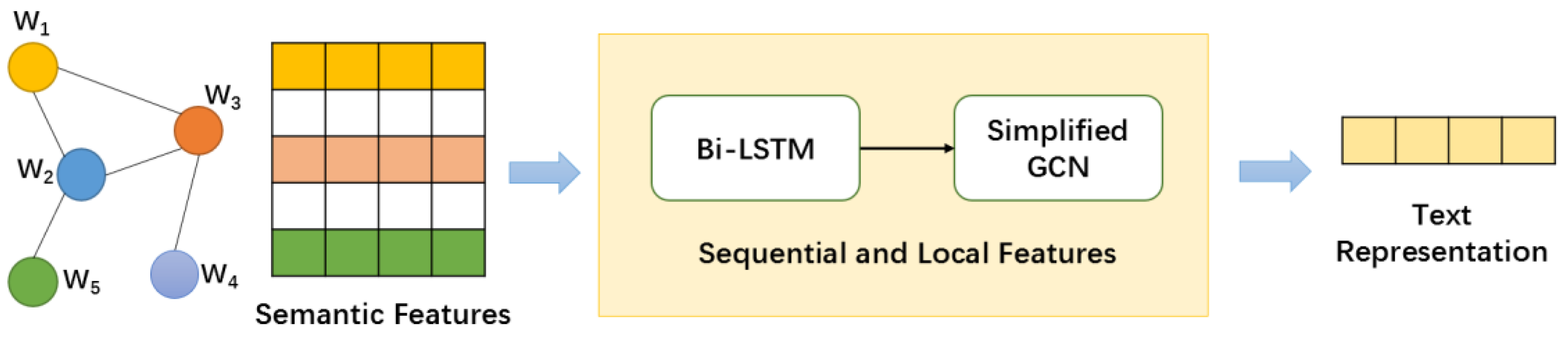
• We propose an improved sequence-based feature propagation scheme. Each document in the corpus is trained as an individual graph, and the sequential features and local features of words in each document are learned, which contributes to the analysis of textual features.
• We propose new GNN-based models, SGNN and ESGNN, for short text classification, combining the Bi-LSTM network and simplified GCNs, which can better understand document semantics and generate more accurate text representation.
• We conduct extensive experiments on seven short text classification datasets with different sentence lengths, and the results show that our approach outperforms state-of-the-art text classification methods.

Figure 1. The whole framework of our method.

Figure 1. The whole framework of our method.

Table 1. The novelty of our work compared with other proposals.

Models	Sequential Information	Structural Information	Inductive Learning
Bi-LSTM	√		√
TextGCN		√
TensorGCN	√	√
S-LSTM		√	√
TextING	√	√	√
Our Model	√	√	√

Table 1. The novelty of our work compared with other proposals.

Models	Sequential Information	Structural Information	Inductive Learning
Bi-LSTM	√		√
TextGCN		√
TensorGCN	√	√
S-LSTM		√	√
TextING	√	√	√
Our Model	√	√	√

The rest of the paper is organized as follows. First, Section 2 introduces our method in detail, which includes graph construction and our proposed models. Second, we describe seven datasets for short text classification, baseline models and experimental settings in detail in Section 3. Section 4 shows the overall test performance of our models and baseline models and reports the experimental results in detail. Finally, we summarize this research and discuss the prospects of future research in Section 5.

2. Methods

In this section, the detailed method is introduced. First, we detail how to construct individual document graphs for each document in the short text corpus. Second, we describe our proposed SGNN model and its extended ESGNN model in detail. Third, we detail how to predict the label for a given text according to the learned representations of documents.

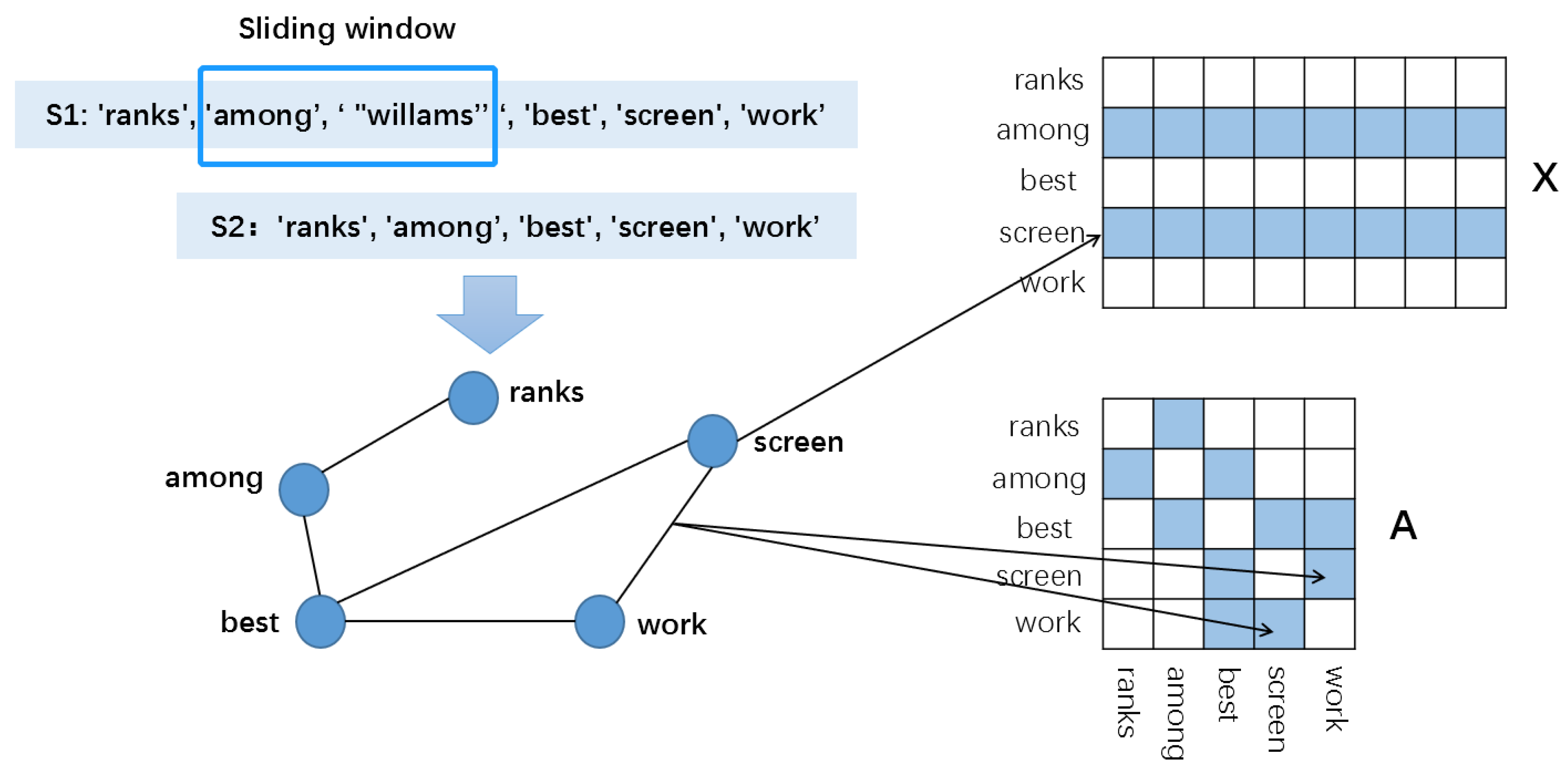
2.1. Graph Construction

We constructed individual graphs for each document in the short text corpus. We represented words as nodes and the co-occurrence relationship between words as edges, denoted as $G=\left(V, E\right)$, where $V$ is the set of nodes and $E$ is the set of edges. First, we preprocessed the text, including cleaning and tokenizing [28], to obtain the word sequence $S1$. Second, we removed the stop words, including the stop words of NLTK (http://www.nltk.org/) (accessed on 30 November 2021) and the words with word frequencies less than 5 in the corpus, to obtain the word sequence $S2$. Third, a fixed-size sliding window (length = 4 at default) was used to generate edges according to word co-occurrence on word sequences $S1$. If the word in the sliding window does not appear in the $S2$ sequence, then delete the node and corresponding edge in the graph. Finally, the embedding of nodes in each document graph were initialized with word embedding, denoted as $X\in R{ }^{\mid V\mid \times d}$, where $d$ is the embedding dimension. An example of constructing a document graph is shown in Figure 2.

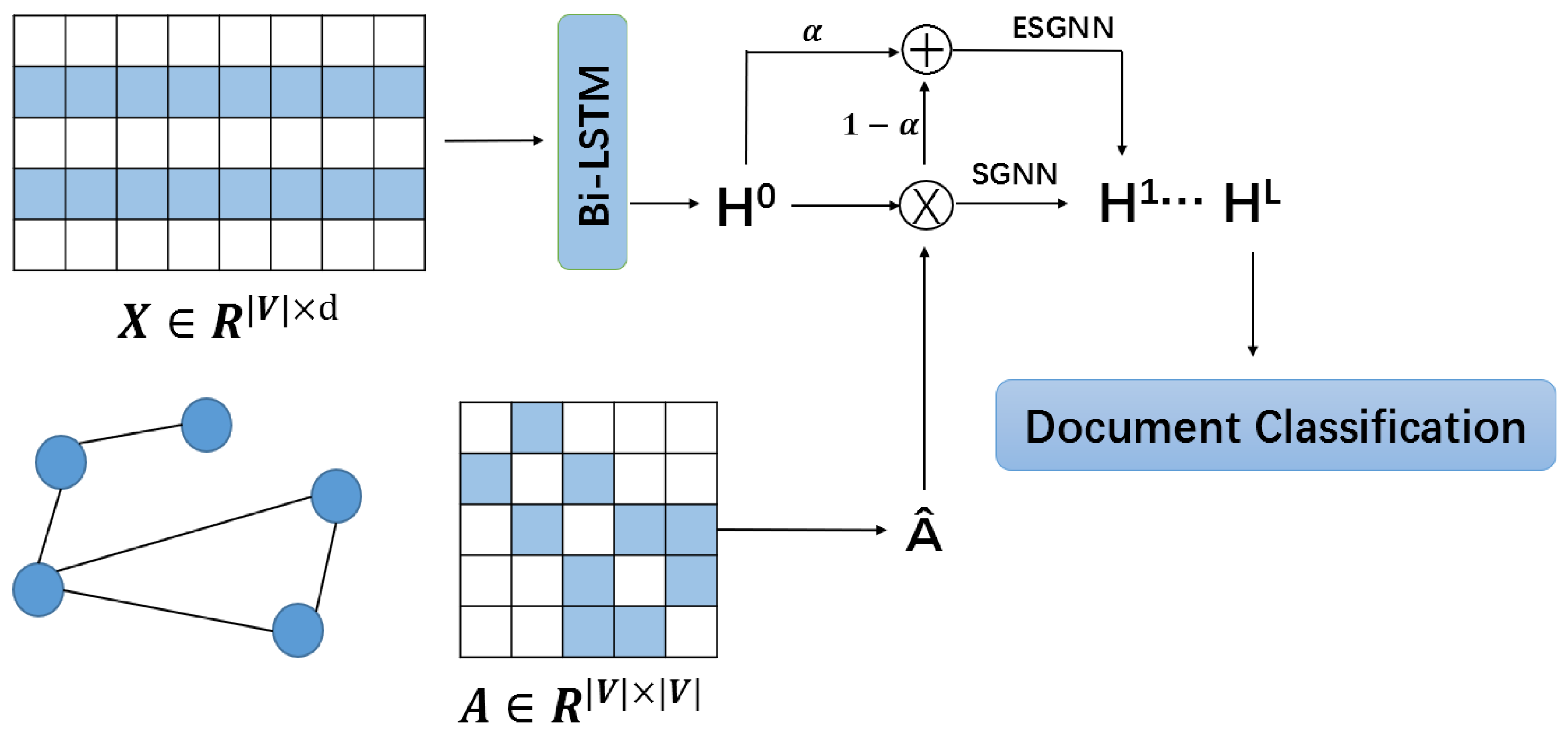
2.2. SGNN Model and ESGNN Model

With the continuous development of GNNs, GCNs are a simple and widely used message passing algorithm for semi-supervised classification [45]. In one message passing layer, GCNs propagate the features of nodes through average aggregation and transform the features of nodes by linear mapping. Its equation is

$$\widehat{A}={\widehat{D}}^{-\frac{1}{2}}\left(A+I_{\mid V\mid }\right){\widehat{D}}^{-\frac{1}{2}}$$

(1)

$$X^{\prime }=\sigma \left(\widehat{A}XW\right)$$

(2)

where $I_{\left|V\right|}$ is the identity matrix, $\widehat{A}={\widehat{D}}^{-\frac{1}{2}}\left(A+I_{\mid V\mid }\right){\widehat{D}}^{-\frac{1}{2}}$ is the symmetrically normalized adjacency matrix with self-loops, with the diagonal degree matrix ${\widehat{D}}_{ij}={{\displaystyle \sum }}_k{\left(A+I_{\mid V\mid }\right)}_{ik}$, $W$ is the trainable weight matrix, $\sigma$ is the activation function, such as ReLU, and $X\in R^{\left|V\right|\times d}$ and $X^{\prime }\in R^{\left|V\right|\times d}$ are the feature matrices of the current layer and next layer, respectively [41].

Recently, it has been found that by decoupling the GCN’s feature transformation and propagation and removing the nonlinearities between GCN layers, the improved GCN is more efficient than the traditional GCN in many tasks [46,47]. Inspired by the above research, we propose SGNN and ESGNN models for short text classification. The model architecture is shown in Figure 3. Since Bi-LSTM can capture bidirectional semantic dependencies, it can well model the sequential information of documents. Therefore, for each document in the short text corpus, Bi-LSTM is used to extract the contextual information between words, learn the unique word representations of each document, and then update the feature matrix of the document graph. Then, we use the simplified GCN to aggregate the features of neighboring nodes on average and update the word node representation. The formulas of the SGNN model are as follows:

$$H^{\left(0\right)}=Bi-LSTM\left(X\right)$$

(3)

$$H^{L+1}=\widehat{A}{H}^{\left(L\right)}$$

(4)

where $H^{\left(L\right)}\in R^{\mid V\mid \times d}$ is the feature matrix of the hidden layer.

In addition, we extend our model with a branch ESGNN, where in the process of node aggregation, through set $\alpha =0.1, 0.2\dots$, the initial contextual feature of words is preserved. The formula of the ESGNN is as follows:

$$H^{L+1}=\left(1-\alpha \right)\widehat{A}{H}^{\left(L\right)}+\alpha H^{\left(0\right)}$$

(5)

2.3. Document Classification

After the word nodes of each document were fully updated, we used global maximum pooling to extract features from the output of the last SGNN or ESGNN layer and obtain the graph-level representation of each document.

$$X_{doc}=MaxPooling\left(H^L\right)$$

(6)

where $X_{doc}\in R^{d^L}$ and L are the layer numbers of the SGNN or the ESGNN model. Finally, the label of the document is predicted by feeding the graph-level embedding $X_{doc}$ into a $softmax$ layer:

$$y_i=softmax\left(X_{doc}{W}_{linear}+b\right)$$

(7)

where $W_{linear}$ and $b$ are weights and bias, respectively. The goal of training is to minimize the cross-entropy loss between ground truth label $y$ and predicted label $y_i$.

$$loss=-ylog{y}_i$$

(8)

3. Materials and Experiments

In this section, we describe our datasets, baseline models, and experimental settings in detail.

3.1. Datasets

We conducted experiments on seven short text datasets, including R8, R52, MR, SearchSnippets, SMS, and Biomedical. The detailed description of each dataset is listed below.

• R52 and R8 are two subsets of the Reuters 21,578 dataset (http://disi.unitn.it/moschitti/corpora.htm) (accessed on 30 November 2021). R8 has 8 categories, which were split to 5485 training and 2189 test documents. R52 has 52 categories, which were split to 6532 training and 2568 test documents.
• Ag News (http://www.di.unipi.it/~gulli/AG_corpus_of_news_articles.html) (accessed on 30 November 2021) is a news dataset from [48], which consists of the following four topics: World, Sports, Business and Sci/Tech. We randomly selected 4000 items from each category to form a dataset for the experiment. In our experiment we called it Ag News Sub.
• MR (https://github.com/mnqu/PTE/tree/master/data/mr) (accessed on 30 November 2021) is a movie review dataset for binary sentiment classification, where each review contains only one sentence [49]. The corpus has 5331 positive and 5331 negative reviews. We used the same training and test set division methods as [50].
• SearchSnippets (http://jwebpro.sourceforge.net/data-web-snippets.tar.gz) (accessed on 30 November 2021) dataset is released by [51], which contains 12,340 documents. It is composed of the search results which based on 8 different domains terms in search engines, including business, computer, health, education, etc.
• SMS (http://www.dt.fee.unicamp.br/~tiago/smsspamcollection/) (accessed on 30 November 2021) is a binary classification dataset collected for short message spam research, which contains 5574 pieces of English, real and unencrypted messages.
• Biomedical is built by [52] from an internationally renowned biomedical platform BioASQ (http://participants-area.bioasq.org/) (accessed on 30 November 2021) and contains 20,000 documents. It consists of 20 categories of titles of the papers that belong to the MeSH theme as the dataset.

We first preprocessed all the datasets by cleaning and tokenizing text as [28]. Then, we deleted stop words defined in NLTK and low-frequency words that appeared less than 5 times for R8, R52, and Ag news sub. For the other four datasets, we did not delete words after cleaning and tokenizing raw text because the documents were very short, so word sequence S1 and word sequence S2 were the same. The statistics of the datasets are shown in

Table 2. Statistics of datasets.

Datasets	Doc	Train	Test	Classes	Avg Length	Max Length
R52	9100	6532	2568	52	69.82	612
R8	7674	5485	2189	8	65.72	520
Ag News Sub	16,000	11,200	4800	4	28.11	146
MR	10,662	7108	3554	2	20.39	56
SearchSnippets	12,340	8636	3704	8	18.10	50
SMS	5574	3900	1674	2	17.11	190
Biomedical	20,000	14,000	6000	20	12.88	53

.

3.2. Baselines

In the experiment, we compared our methods with the different state-of-the-art models. The models used in the experiment are as follows.

• TextCNN [28]: We implemented TextCNN, which uses pretrained word embedding and fine-tuning during the training process, and we set the kernals’ size with (3, 4, 5).
• Bi-LSTM [29]: a bidirectional LSTM that is commonly used in text classification. We input pretrained word embedding to Bi-LSTM.
• Fasttext [52]: A simple and efficient text classification method that takes the average of all word embedding as document representation and then feeds the document representation into a linear classifier. We evaluated it without bigrams.
• SWEM: A simple word embedding model proposed by [53], and in our experiment, we used SWEM-concat and obtained the final text representation through two fully connected layers.
• TextGCN: A graph-based text classification model proposed by [35], which builds a single large graph for the whole corpus and converts text classification into a node classification task based on GCN.
• TensorGCN: A graph-based text classification model in [40], which uses semantic and syntactic contextual information.
• HeteGCN [54]: A model unites the best aspects of predictive text embedding and TextGCN together.
• S-LSTM [37]: A model that treats each sentence or document as a graph and uses repeated steps to exchange local and global information between word nodes at the same time.
• TextING [41]: This model builds individual graphs for each document and uses a gated graph neural network to learn word interactions at the text level.

3.3. Experiment Settings

For all the datasets, we randomly split the training set into a ratio of 9:1 for actual training and validation. We used pretrained 300-dimensional GloVe (http://nlp.stanford.edu/data/glove.6B.zip) (accessed on 30 November 2021) word embedding as the input features, whereas the out-of-vocabulary (OOV) words were set to 0. We referred to [55] and used a maximum sentence length as the truncation for SearchSnippets, Biomedical, and MR, whereas Ag New Sub and SMS were set to 50, and R8 and R52 were set to 100. Empirically, the batch size of our model was 32, the number of layers and the hidden length of Bi-LSTM were 2 and 128, respectively, the learning rate was 0.002 with the Adam [4,56] optimizer, and the dropout rate was 0.5. For learning SGNN and ESGNN, we trained the model for 100 epochs with an early stopping strategy. For baseline models, we used the default parameter settings as in their original papers or implementations. For models using pretrained word embedding, we used 300-dimensional GloVe word embedding.

4. Results and Discussion

In this section, we describe experimental results in detail, and to further analyze our models, we explore the influence of different parameters on the model’s ability in the experiment.

4.1. Test Performance

Table 3. Test accuracy (%) for various models on different datasets. We ran all models 10 times and reported the average ± standard deviation as the experimental result. Best results are shown in bold.

Models	R8	R52	Agnewssub	MR	Searchsnippets	SMS	Biomedical
TextCNN	95.71 ± 0.52	87.59 ± 0.48	88.74 ± 0.16	77.75 ± 0.72	89.52 ± 0.35	99.03 ± 0.05	73.08 ± 0.33
Bi-LSTM	96.31 ± 0.33	90.54 ± 0.91	87.68 ± 0.35	77.68 ± 0.86	84.81 ± 1.40	98.77 ± 0.10	63.42 ± 0.97
fastText	96.13 ± 0.21	92.81 ± 0.09	88.22 ± 0.04	75.14 ± 0.20	88.56 ± 0.12	98.84 ± 0.06	65.17 ± 0.22
SWEM	95.32 ± 0.26	92.94 ± 0.24	87.77 ± 0.05	76.65 ± 0.63	87.36 ± 0.32	98.33 ± 0.11	68.97 ± 0.20
TextGCN	97.07 ± 0.10	93.56 ± 0.18	87.55 ± 0.10	76.74 ± 0.20	83.49 ± 0.20	98.30 ± 0.05	69.67 ± 0.20
TensorGCN	98.04 ± 0.08	95.05 ± 0.11	-	77.91 ± 0.07	-	-	-
S-LSTM	97.67 ± 0.14	94.92 ± 0.19	88.21 ± 0.38	77.75 ± 0.31	87.54 ± 0.33	98.60 ± 0.08	73.77 ± 0.20
TextING	98.04 ± 0.25	95.48 ± 0.19	89.24 ± 0.20	79.82 ± 0.20	87.03 ± 0.43	98.89 ± 0.19	73.88 ± 0.50
SGNN	98.09 ± 0.08	95.46 ± 0.15	89.57 ± 0.25	80.58 ± 0.18	90.68 ± 0.32	99.22 ± 0.11	74.92 ± 0.34
ESGNN	98.23 ± 0.09	95.72 ± 0.16	89.66 ± 0.18	80.93 ± 0.14	90.80 ± 0.21	99.31 ± 0.06	75.34 ± 0.36

and

Table 4. Test Macro-F1 (%) for various models on different datasets. We ran all models 10 times and reported the average as the experimental result. Best results are shown in bold.

Models	R8	R52	Agnewssub	MR	Searchsnippets	SMS	Biomedical
TextCNN	93.24	60.93	88.14	77.25	88.12	97.21	71.95
Bi-LSTM	93.68	63.10	87.06	77.13	83.62	96.91	60.08
fastText	90.76	57.98	88.10	74.45	87.33	95.67	60.55
SWEM	89.29	48.27	86.98	75.67	87.06	95.42	68.19
TextGCN	93.38	67.79	86.88	76.24	82.74	95.62	69.76
HeteGCN	92.33	66.53	-	75.62	-	-	-
S-LSTM	93.80	73.33	87.44	76.96	86.63	96.03	71.53
TextING	93.62	73.38	88.89	79.02	86.26	97.19	72.14
ESGNN	94.31	74.54	88.95	79.83	89.10	97.87	73.02

show the test accuracy and test macro-f1 of all baselines and our two models for all datasets, respectively. We can see that our model achieves optimal results on all datasets, especially for datasets with short average text lengths, such as Ag news sub, MR, Searchsnippets, SMS, and Biomedical. SSGNN has performed better than other baselines, which proves the effectiveness of our method on short text datasets. In addition, ESGNN performs better than SGNN, which shows that the feature extraction ability of the model is more powerful for short text classification. Moreover, we also evaluate the model efficiency by the training time of per epoch, as shown in

Table 5. Training time (minutes) per epoch of GNN-based models.

Dataset	TextGCN	TensorGCN	S-LSTM	TextING	SGNN	ESGNN
MR	1.72	3.34	8.09	2.58	2.42	2.50
R52	2.64	4.32	10.65	4.98	3.19	3.24

; it can be seen that in addition to TextGCN, our method shows better advantages compared with other GNN-based methods, which may be because TextGCN builds a large corpus graph and only captures the structural information of each document.

We note that TextGCN based on a large corpus graph model performs better than traditional models such as CNN and RNN in R8 and R52. This may be because the average texts length of R8 and R52 is relatively long. TextGCN can capture global word co-occurrence in the long-distance corpus by constructing a single large graph and take advantage of GCN in dealing with complex network structure to learn more accurate representations of document nodes. We also note that S-LSTM and TextING based on small graphs perform better than traditional models, which may be because traditional models lack long-distance and non-consecutive word interactions [41]. In addition, they also perform better than TextGCN based on a large corpus graph model. This may be because small graph excludes a large number of words that are far away in the text and have little relationship with the current words [36] to learn more accurate text representation in a specific context, so the generalization ability of the model is further improved. Additionally, both of them make use of the advantage of pretrained word embedding and achieve better results.

Our model performs better than the traditional models and also better than the most advanced graph models, such as S-LSTM and TextING. This may be because our model first captures the continuous semantic information of the document to well model the sequential information of the document, which is considered in the feature matrix of each document graph. In addition, taking advantage of small graphs, local structure features of word nodes are extracted by using the dependency relationship between the word nodes in the document. In summary, our method uses the semantic features of the pretrained word embedding and document-level word interaction, which extracts the sequential information and structural information of each document, to improve the classification accuracy. It has powerful feature extraction and text representation abilities and achieves better classification performance in short text classification.

4.2. Combine with Bert

One of the advantages of the pre-trained model is that it can obtain contextual dynamic word embedding, which shows better results than the static word embedding in NLP tasks [32]. Therefore, we use Bert instead of Bi-LSTM as the input of the model to explore the combination ability of our method with Bert, which is called C-Bert. The formulas of the C-Bert model are as follows:

$$X^{bert}=Bert\left(S\right)$$

(9)

$$H^{L+1}=\left(1-\alpha \right)\widehat{A}{H}^{\left(L\right)}+\alpha X^{bert}$$

(10)

where $S$ is the word sequence of each document in the short text corpus.

The experimental results are shown in

Table 6. Comparison of models based on Bert.

Models	R8	R52	Agnewssub	MR	Searchsnippets	SMS	Biomedical
ESGNN	98.23 ± 0.09	95.72 ± 0.16	89.66 ± 0.18	80.93 ± 0.14	90.80 ± 0.21	99.31 ± 0.06	75.34 ± 0.36
BERT	98.07 ± 0.13	95.79 ± 0.07	90.02 ± 0.23	85.86 ± 0.16	90.15 ± 0.11	99.40 ± 0.05	72.60 ± 0.33
C-BERT	98.28 ± 0.39	96.52 ± 0.85	90.36 ± 0.40	86.06 ± 0.73	90.43 ± 0.60	99.36 ± 0.08	74.15 ± 0.66

. It shows that Bert is better than our model on the five datasets except for Searchsnippets and Biomedical, which may be because of the words out of vocabulary. Moreover, we can find that in addition to SMS, the C-Bert model shows better results than Bert, which proves the effectiveness of our feature propagation scheme.

4.3. Parameter Sensitivity Analysis

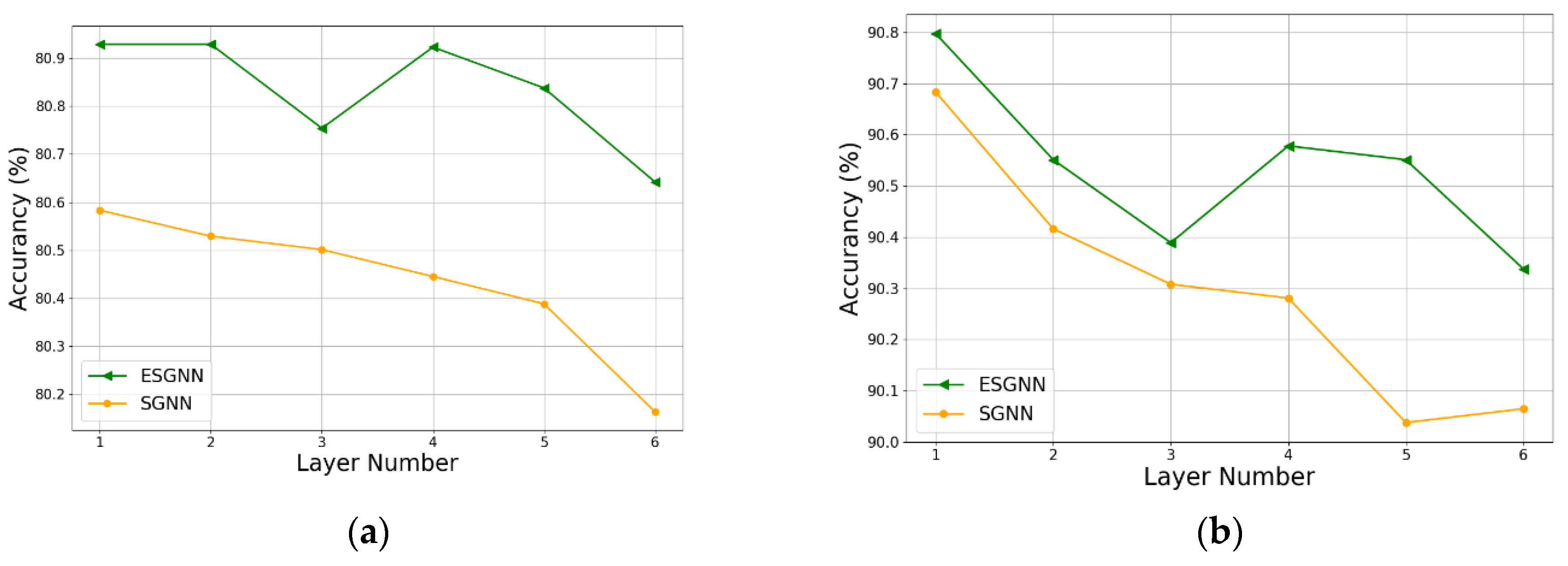
4.3.1. Graph Layers

Figure 4 shows the test performance of our two models using different graph layers on MR and Searchsnippets. The results reveal that when L = 1, the test results of the two datasets are optimal, which shows that the models capture the textual features of each document in the short text corpus well. However, with the increase in the number of layers, both of the models present a different downward trend in different datasets. This may be because of the short average text length in a short text corpus; for word nodes in each document graph, too much received information from high-order neighbors will make the word nodes become overly smooth, which inhibits the generalization ability of the model. In addition, ESGNN performs better than SGNN with the number of layers increasing, which indicates that in the process of node aggregation, preserving proper initial contextual feature information is helpful to alleviate the over-smoothing problem.

4.3.2. Slide Window Sizes

Figure 5 shows the effect of different window sizes on the performance of the SGNN model in MR and Searchsnippets. The generalization ability of the model increases with increasing window size, and each word node has more neighbors, which increases the scope of feature exchange to learn the representation of word nodes more accurately. For both datasets, the model obtains the best results when the window size is equal to 4. However, when the window size is larger than 4, the performance of different datasets shows a different downward trend. This may be because large window sizes may not introduce very close edges for word nodes, resulting in excessive feature exchange.

4.3.3. Probability of $\mathsf{\alpha }$

Figure 6 shows the effect of using different values of α on the performance of the ESGNN model in R52 and Biomedical. The results show that when the α value increases, the trend is similar to window sizes, and the optimum typically lies within α ∈ [0.2, 0.3] but slightly changes for different datasets. The value should be adjusted according to the dataset since the average text length of different datasets is different, and different document graphs exhibit different neighborhood structures [57,58]. In addition, compared with SGNN (the dotted orange line in the figure), we note that too small or too large values will affect the structure information during aggregation, which reduces the feature extraction ability of the ESGNN model.

4.3.4. Proportions of Training Data

GCNs can perform well with a low label rate during training [45]; therefore, to test the robustness of the model for semi-supervised tasks [59], we use different proportions of training datasets to test graph-based models. For MR and SMS, we reduce the training data to 1%, 2.5%, 5%, 10%, 15% and 20%, respectively. Figure 7 shows the test results of ESGNN, SGNN, TextING, S-LSTM, and TextGCN. We note that with the increase in training data, our ESGNN and SGNN models perform better than TextING, S-LSTM, and TextGCN in most cases. The extraction of sequential features also helps to generate a more accurate representation for the word nodes of the test set, which do not appear in the training set, and gives our model stronger feature extraction and text representation abilities in limited training labeled documents.

5. Conclusions

In this work, we propose an improved sequence-based feature propagation scheme that can better analyze textual features. We also propose a new GNN-based method for short text classification, termed SGNN, and its extended model, ESGNN. Each document in the short text corpus is trained as an individual graph; our two models extract the sequential features and structural features of each document in turn from the semantic features of words, which increases the feature exchange between words in the document and overcomes the limitations of textual features in short texts, and the accuracy of short text classification is improved. Moreover, experimental results suggest the strong robustness of our models to less training data compared with other graph-based models. In future work, we will explore more effective feature propagation schemes and propose more effective models to improve the adaptability of the model to different classification tasks in NLP.

References

1. Song, G.; Ye, Y.; Du, X.; Huang, X.; Bie, S. Short Text Classification: A Survey. J. Multimed. 2014, 9, 635–643. [Google Scholar] [CrossRef]
2. Elnagar, A.; Al-Debsi, R.; Einea, O. Arabic text classification using deep learning models. Inf. Process. Manag. 2020, 57, 102121. [Google Scholar] [CrossRef]
3. Tadesse, M.M.; Lin, H.; Xu, B.; Yang, L. Detection of suicide ideation in social media forums using deep learning. Algorithms 2020, 13, 7. [Google Scholar] [CrossRef] [Green Version]
4. Kingma, D.P.; Ba, J.L. Adam: A Method for Stochastic Optimization. In Proceedings of the International Conference on Learning Representations, San Diego, CA, USA, 7–9 May 2015. [Google Scholar]
5. Meng, Y.; Shen, J.; Zhang, C.; Han, J. Weakly-Supervised Neural Text Classification. In Proceedings of the Conference on Information and Knowledge Management, Turin, Italy, 22–26 October 2018; pp. 983–992. [Google Scholar]
6. Chen, Q.; Hu, Q.; Huang, J.X.; He, L.; An, W. Enhancing Recurrent Neural Networks with Positional Attention for Question Answering. In Proceedings of the International ACM SIGIR Conference on Research and Development in Information Retrieval, Tokyo, Japan, 7–21 August 2017; pp. 993–996. [Google Scholar]
7. Elnagar, A.; Lulu, L.; Einea, O. An Annotated Huge Dataset for Standard and Colloquial Arabic Reviews for Subjective Sentiment Analysis. Procedia Comput. Sci. 2018, 142, 182–189. [Google Scholar] [CrossRef]
8. Pintelas, P.; Livieris, I.E. Special issue on ensemble learning and applications. Algorithms 2020, 13, 140. [Google Scholar] [CrossRef]
9. Forman, G. BNS feature scaling: An improved representation over tf-idf for svm text classification. In Proceedings of the Conference on Information and Knowledge Management, Napa Valley, CA, USA, 26–30 October 2008; pp. 263–270. [Google Scholar]
10. Zuo, Y.; Wu, J.; Zhang, H.; Lin, H.; Wang, F.; Xu, K.; Xiong, H. Topic Modeling of Short Texts: A Pseudo-Document View. In Proceedings of the Knowledge Discovery and Data Mining, San Francisco, CA, USA, 13–17 August 2016; pp. 2105–2114. [Google Scholar]
11. Wang, S.; Manning, C. Baselines and Bigrams: Simple, Good Sentiment and Topic Classification. In Proceedings of the Meeting of the Association for Computational Linguistics, Jeju, Korea, 8–14 July 2012; pp. 90–94. [Google Scholar]
12. Zhang, Y.; Jin, R.; Zhou, Z.H. Understanding bag-of-words model: A statistical framework. Int. J. Mach. Learn. Cybern. 2010, 1, 43–52. [Google Scholar] [CrossRef]
13. Mouratidis, D.; Kermanidis, K.L. Ensemble and deep learning for language-independent automatic selection of parallel data. Algorithms 2019, 12, 26. [Google Scholar] [CrossRef] [Green Version]
14. Le, Q.; Mikolov, T. Distributed Representations of Sentences and Documents. In Proceedings of the International Conference on Machine Learning, Beijing, China, 21–26 June 2014; pp. 1188–1196. [Google Scholar]
15. Cunha, W.; Mangaravite, V.; Gomes, C.; Canuto, S.; Resende, E.; Nascimento, C.; Viegas, F.; França, C.; Martins, W.S.; Almeida, J.M. On the cost-effectiveness of neural and non-neural approaches and representations for text classification: A comprehensive comparative study. Inf. Process. Manag. 2021, 58, 102481. [Google Scholar] [CrossRef]
16. Devlin, J.; Chang, M.-W.; Lee, K.; Toutanova, K.N. BERT: Pre-training of Deep Bidirectional Transformers for Language Understanding. In Proceedings of the North American Chapter of the Association for Computational Linguistics, New Orleans, LA, USA, 1–8 June 2018; pp. 4171–4186. [Google Scholar]
17. Zheng, J.; Cai, F.; Chen, H.; Rijke, M.d. Pre-train, Interact, Fine-tune: A novel interaction representation for text classification. Inf. Process. Manag. 2020, 57, 102215. [Google Scholar] [CrossRef] [Green Version]
18. Muaad, A.Y.; Jayappa, H.; Al-antari, M.A.; Lee, S. ArCAR: A Novel Deep Learning Computer-Aided Recognition for Character-Level Arabic Text Representation and Recognition. Algorithms 2021, 14, 216. [Google Scholar] [CrossRef]
19. McCann, B.; Bradbury, J.; Xiong, C.; Socher, R. Learned in translation: Contextualized word vectors. In Proceedings of the Neural Information Processing Systems, Long Beach, CA, USA, 4–9 December 2017; pp. 6297–6308. [Google Scholar]
20. Peters, M.E.; Neumann, M.; Iyyer, M.; Gardner, M.; Clark, C.; Lee, K.; Zettlemoyer, L. Deep contextualized word representations. In Proceedings of the North American Chapter of the Association for Computational Linguistics, New Orleans, LA, USA, 1–8 June 2018; pp. 2227–2237. [Google Scholar]
21. Mikolov, T.; Chen, K.; Corrado, G.S.; Dean, J. Efficient Estimation of Word Representations in Vector Space. In Proceedings of the International Conference on Learning Representations, Scottsdale, AZ, USA, 2–4 May 2013. [Google Scholar]
22. Mikolov, T.; Sutskever, I.; Chen, K.; Corrado, G.S.; Dean, J. Distributed Representations of Words and Phrases and their Compositionality. In Proceedings of the Neural Information Processing Systems, Lake Tahoe, NV, USA, 5–10 December 2013; pp. 3111–3119. [Google Scholar]
23. Pennington, J.; Socher, R.; Manning, C. Glove: Global Vectors for Word Representation. In Proceedings of the Empirical Methods in Natural Language Processing, Doha, Qatar, 25–29 October 2014; pp. 1532–1543. [Google Scholar]
24. Sanchez-Reyes, L.M.; Rodriguez-Resendiz, J.; Avecilla-Ramirez, G.N.; Garcia-Gomar, M.L.; Robles-Ocampo, J.B. Impact of EEG Parameters Detecting Dementia Diseases: A Systematic Review. IEEE Access 2021, 9, 78060–78074. [Google Scholar] [CrossRef]
25. Ortiz-Echeverri, C.J.; Salazar-Colores, S.; Rodríguez-Reséndiz, J.; Gómez-Loenzo, R.A. A new approach for motor imagery classification based on sorted blind source separation, continuous wavelet transform, and convolutional neural network. Sensors 2019, 19, 4541. [Google Scholar] [CrossRef] [PubMed] [Green Version]
26. Villegas-Mier, C.G.; Rodriguez-Resendiz, J.; Álvarez-Alvarado, J.M.; Rodriguez-Resendiz, H.; Herrera-Navarro, A.M.; Rodríguez-Abreo, O. Artificial Neural Networks in MPPT Algorithms for Optimization of Photovoltaic Power Systems: A Review. Micromachines 2021, 12, 1260. [Google Scholar] [CrossRef] [PubMed]
27. Gutierrez-Villalobos, J.M.; Rodriguez-Resendiz, J.; Rivas-Araiza, E.A.; Mucino, V.H. A review of parameter estimators and controllers for induction motors based on artificial neural networks. Neurocomputing 2013, 118, 87–100. [Google Scholar] [CrossRef]
28. Kim, Y. Convolutional Neural Networks for Sentence Classification. In Proceedings of the Empirical Methods in Natural Language Processing, Doha, Qatar, 25–29 October 2014; pp. 1746–1751. [Google Scholar]
29. Liu, P.; Qiu, X.; Huang, X. Recurrent neural network for text classification with multi-task learning. In Proceedings of the International Joint Conference on Artificial Intelligence, New York, NY, USA, 9–15 July 2016; pp. 2873–2879. [Google Scholar]
30. Battaglia, P.W.; Hamrick, J.B.; Bapst, V.; Sanchez-Gonzalez, A.; Zambaldi, V.; Malinowski, M.; Tacchetti, A.; Raposo, D.; Santoro, A.; Faulkner, R. Relational inductive biases, deep learning, and graph networks. arXiv 2018, arXiv:1806.01261. [Google Scholar]
31. Cliche, M. BB_twtr at SemEval-2017 Task 4: Twitter Sentiment Analysis with CNNs and LSTMs. In Proceedings of the Meeting of the Association for Computational Linguistics, Vancouver, BC, Canada, 30 July–4 August 2017; pp. 573–580. [Google Scholar]
32. Sun, C.; Qiu, X.; Xu, Y.; Huang, X. How to Fine-Tune BERT for Text Classification? In Proceedings of the China National Conference on Chinese Computational Linguistics, Kunming, China, 18–20 October 2019. [Google Scholar]
33. Garg, S.; Ramakrishnan, G. BAE: BERT-based Adversarial Examples for Text Classification. In Proceedings of the The 2020 Conference on Empirical Methods in Natural Language Processing (EMNLP), Online, 16–20 November 2020. [Google Scholar]
34. Zhou, J.; Cui, G.; Zhang, Z.; Yang, C.; Liu, Z.; Wang, L.; Li, C.; Sun, M. Graph neural networks: A review of methods and applications. arXiv 2018, arXiv:1812.08434. [Google Scholar] [CrossRef]
35. Yao, L.; Mao, C.; Luo, Y. Graph Convolutional Networks for Text Classification. In Proceedings of the AAAI Conference on Artificial Intelligence, Honolulu, HI, USA, 27 July–1 February 2019; pp. 7370–7377. [Google Scholar]
36. Huang, L.; Ma, D.; Li, S.; Zhang, X.; Wang, H. Text Level Graph Neural Network for Text Classification. In Proceedings of the Empirical Methods in Natural Language Processing, Hong Kong, China, 3–7 November 2019; pp. 3442–3448. [Google Scholar]
37. Zhang, Y.; Liu, Q.; Song, L. Sentence-State LSTM for Text Representation. In Proceedings of the Meeting of the Association for Computational Linguistics, Melbourne, Australia, 15–20 July 2018; pp. 317–327. [Google Scholar]
38. Mihalcea, R.; Tarau, P. TextRank: Bringing Order into Text. In Proceedings of the Empirical Methods in Natural Language Processing, Barcelona, Spain, 25–26 July 2004; pp. 404–411. [Google Scholar]
39. Ding, K.; Wang, J.; Li, J.; Li, D.; Liu, H. Be More with Less: Hypergraph Attention Networks for Inductive Text Classification. In Proceedings of the 2020 Conference on Empirical Methods in Natural Language Processing (EMNLP), Online, 16–20 November 2020. [Google Scholar] [CrossRef]
40. Liu, X.; You, X.; Zhang, X.; Wu, J.; Lv, P. Tensor Graph Convolutional Networks for Text Classification. In Proceedings of the AAAI Conference on Artificial Intelligence, New York, NY, USA, 1–12 February 2020; pp. 8409–8416. [Google Scholar]
41. Zhang, Y.; Yu, X.; Cui, Z.; Wu, S.; Wen, Z.; Wang, L. Every Document Owns Its Structure: Inductive Text Classification via Graph Neural Networks. In Proceedings of the Meeting of the Association for Computational Linguistics, Online, 6–8 July 2020; pp. 334–339. [Google Scholar]
42. Peng, H.; Li, J.; He, Y.; Liu, Y.; Bao, M.; Wang, L.; Song, Y.; Yang, Q. Large-Scale Hierarchical Text Classification with Recursively Regularized Deep Graph-CNN. In Proceedings of the The Web Conference, Lyon, France, 23–27 April 2018; pp. 1063–1072. [Google Scholar]
43. Abdi, A.; Shamsuddin, S.M.; Hasan, S.; Piran, J. Deep learning-based sentiment classification of evaluative text based on Multi-feature fusion. Inf. Process. Manag. 2019, 56, 1245–1259. [Google Scholar] [CrossRef]
44. Liu, Y.; Meng, F.; Chen, Y.; Xu, J.; Zhou, J. Depth-Adaptive Graph Recurrent Network for Text Classification. arXiv 2020, arXiv:2003.00166. [Google Scholar]
45. Kipf, T.N.; Welling, M. Semi-Supervised Classification with Graph Convolutional Networks. In Proceedings of the International Conference on Learning Representations, San Juan, Puerto Rico, 2–4 May 2016. [Google Scholar]
46. Wu, F.; Souza, A.H.; Zhang, T.; Fifty, C.; Yu, T.; Weinberger, K.Q. Simplifying Graph Convolutional Networks. In Proceedings of the International Conference on Machine Learning, Long Beach, CA, USA, 9–15 June 2019; pp. 6861–6871. [Google Scholar]
47. Chen, M.; Wei, Z.; Huang, Z.; Ding, B.; Li, Y. Simple and Deep Graph Convolutional Networks. In Proceedings of the International Conference on Machine Learning, Online, 13–18 July 2020; pp. 1725–1735. [Google Scholar]
48. Zhang, X.; Zhao, J.; LeCun, Y. Character-level convolutional networks for text classification. In Proceedings of the Neural Information Processing Systems, Montreal, QC, Canada, 7–12 December 2015; pp. 649–657. [Google Scholar]
49. Pang, B.; Lee, L. Seeing Stars: Exploiting Class Relationships for Sentiment Categorization with Respect to Rating Scales. In Proceedings of the Meeting of the Association for Computational Linguistics, Ann Arbor, MI, USA, 25–30 June 2005; pp. 115–124. [Google Scholar]
50. Tang, J.; Qu, M.; Mei, Q. PTE: Predictive Text Embedding through Large-scale Heterogeneous Text Networks. In Proceedings of the Knowledge Discovery and Data Mining, Sydney, Australia, 10–13 August 2015; pp. 1165–1174. [Google Scholar]
51. Xu, J.; Xu, B.; Wang, P.; Zheng, S.; Tian, G.; Zhao, J. Self-Taught convolutional neural networks for short text clustering. Neural Netw. 2017, 88, 22–31. [Google Scholar] [CrossRef] [PubMed] [Green Version]
52. Joulin, A.; Grave, E.; Bojanowski, P.; Mikolov, T. Bag of Tricks for Efficient Text Classification. In Proceedings of the Conference of the European Chapter of the Association for Computational Linguistics, Valencia, Spain, 3–7 April 2017; pp. 427–431. [Google Scholar]
53. Shen, D.; Wang, G.; Wang, W.; Min, M.R.; Su, Q.; Zhang, Y.; Li, C.; Henao, R.; Carin, L. Baseline Needs More Love: On Simple Word-Embedding-Based Models and Associated Pooling Mechanisms. In Proceedings of the Meeting of the Association for Computational Linguistics, Melbourne, Australia, 15–20 July 2018; pp. 440–450. [Google Scholar]
54. Ragesh, R.; Sellamanickam, S.; Iyer, A.; Bairi, R.; Lingam, V. Hetegcn: Heterogeneous graph convolutional networks for text classification. In Proceedings of the Proceedings of the 14th ACM International Conference on Web Search and Data Mining, Jerusalem, Israel, 8–12 March 2021; pp. 860–868. [Google Scholar]
55. Gao, H.; Chen, Y.; Ji, S. Learning Graph Pooling and Hybrid Convolutional Operations for Text Representations. In Proceedings of the The Web Conference, San Francisco, CA, USA, 13–17 May 2019; pp. 2743–2749. [Google Scholar]
56. Landro, N.; Gallo, I.; La Grassa, R. Combining Optimization Methods Using an Adaptive Meta Optimizer. Algorithms 2021, 14, 186. [Google Scholar] [CrossRef]
57. Grover, A.; Leskovec, J. node2vec: Scalable Feature Learning for Networks. In Proceedings of the Knowledge Discovery and Data Mining, San Francisco, CA, USA, 13–17 August 2016; pp. 855–864. [Google Scholar]
58. Abu-El-Haija, S.; Perozzi, B.; Al-Rfou, R.; Alemi, A.A. Watch Your Step: Learning Node Embeddings via Graph Attention. In Proceedings of the Neural Information Processing Systems, Montreal, QC, Canada, 2–8 December 2018; pp. 9180–9190. [Google Scholar]
59. Linmei, H.; Yang, T.; Shi, C.; Ji, H.; Li, X. Heterogeneous Graph Attention Networks for Semi-supervised Short Text Classification. In Proceedings of the Empirical Methods in Natural Language Processing, Hong Kong, China, 3–7 November 2019; pp. 4820–4829. [Google Scholar]
Figure 2. An illustration of constructing a document graph for a real document. S 1 and S 2 represent the word sequence after preprocessing and after removing the stop words, respectively. We set the sliding window size k = 2 in the figure for convenience. A and X represent adjacency matrix and feature matrix, respectively.
Algorithms 14 00352 g002
Figure 3. The architecture of SGNN and ESGNN model. X represents feature matrix. A and A ^ represents adjacency matrix and symmetrically normalized adjacency matrix, respectively. H L is the output of model’s hidden layer.
Algorithms 14 00352 g003
Figure 4. (a) Test accuracy by different SGNN and ESGNN layers for MR; (b) test accuracy by different SGNN and ESGNN layers for Searchsnippets.
Algorithms 14 00352 g004
Figure 5. Test accuracy by different slide window sizes for SGNN. (a) Test accuracy for MR; (b) test accuracy for SearchSnippets.
Algorithms 14 00352 g005
Figure 6. Test accuracy by different values of α for SGNN. (a) Test accuracy for R52; (b) test accuracy for Biomedical.
Algorithms 14 00352 g006
Figure 7. (a) Test accuracy by different training data ratio for MR; (b) test accuracy by different training data ratio for SMS.
Algorithms 14 00352 g007