Robust Bilinear Probabilistic Principal Component Analysis

Abstract

Principal component analysis (PCA) is one of the most popular tools in multivariate exploratory data analysis. Its probabilistic version (PPCA) based on the maximum likelihood procedure provides a probabilistic manner to implement dimension reduction. Recently, the bilinear PPCA (BPPCA) model, which assumes that the noise terms follow matrix variate Gaussian distributions, has been introduced to directly deal with two-dimensional (2-D) data for preserving the matrix structure of 2-D data, such as images, and avoiding the curse of dimensionality. However, Gaussian distributions are not always available in real-life applications which may contain outliers within data sets. In order to make BPPCA robust for outliers, in this paper, we propose a robust BPPCA model under the assumption of matrix variate t distributions for the noise terms. The alternating expectation conditional maximization (AECM) algorithm is used to estimate the model parameters. Numerical examples on several synthetic and publicly available data sets are presented to demonstrate the superiority of our proposed model in feature extraction, classification and outlier detection.

1. Introduction

High-dimensional data are increasingly collected for a variety of applications in the real world. However, high-dimensional data are not often distributed uniformly in their ambient space, instead of that the interesting structure inside the data often lies in a low-dimensional space [1]. One of the fundamental challenges is how to find the low-dimensional data representation for high-dimensional observed data in pattern recognition, machine learning and statistics [2,3]. Principal component analysis (PCA) [4] is arguably the most well-known dimension reduction method for high-dimensional data analysis, and it aims to find the first few principal eigenvectors corresponding to the first few largest eigenvalues of the covariance matrix, and then projects the high-dimensional data onto the low-dimensional subspace spanned by these principal eigenvectors to achieve the purpose of dimensionality reduction.

The traditional PCA is concerned with vectorial data, i.e., 1-D data. For 2-D image trained sample matrices, it is usual to first convert 2-D image matrices into 1-D image vectors. This transformation leads to higher dimensional image sample vectors and a larger covariance matrix, and thus suffers from the difficulty of accurately evaluating the principal eigenvectors of the large scale covariance matrix. Furthermore, such vectorizing of 2-D data destroys the natural matrix structure, and ignores potentially valuable information about the spatial relationships among 2-D data. Therefore, two-dimensional PCA (2DPCA) type algorithms [5,6,7] are proposed to compute principal component weight matrices directly based on 2-D image training with sample matrices instead of using vectorization.

These conventional PCA and 2DPCA algorithms are both derived and interpreted in the standard algebraic framework, thus they lack capability in handling issues of statistical inference or missing data. To remedy these drawbacks, a probabilistic PCA model (PPCA) has been proposed by Tipping and Bishop in [8], which is processed by assuming some Gaussian distributions on observations with introduced extra latent variables, and it has been successfully applied in many machine learning tasks [9]. Following PPCA, a probabilistic second-order PCA, called PSOPCA, is developed in [10] to directly model 2-D image matrices based on the so-called matrix variate Gaussian distributions.

Throughout this paper, ${\mathbb{R}}^{n\times m}$ is the set of all $n\times m$ real matrices, $I_n$ and $0_{m\times n}$ are the $n\times n$ identity matrix and $m\times n$ zero matrix, respectively. The superscript “${·}^T$” means transpose only, ${\parallel ·\parallel }_2$ and ${\parallel ·\parallel }_F$ denote the ${\ell }_2$-norm and Frobenius norm of a matrix, respectively. Denoted by ${\mathcal{N}}_{d_c,d_r}(M,{\Omega }_c,{\Omega }_r)$ is the matrix variate Gaussian distribution [11] with the mean matrix $M\in {\mathbb{R}}^{d_c\times d_r}$, column covariance ${\Omega }_c\in {\mathbb{R}}^{d_c\times d_c}$ and row covariance ${\Omega }_r\in {\mathbb{R}}^{d_r\times d_r}$. A random matrix $X\in {\mathbb{R}}^{d_c\times d_r}$ is said to follow the matrix variate Gaussian distribution ${\mathcal{N}}_{d_c,d_r}(M,{\Omega }_c,{\Omega }_r)$, i.e.,

$$X\sim {\mathcal{N}}_{d_c,d_r}(M,{\Omega }_c,{\Omega }_r),ifvec(X)\sim \mathcal{N}(vec(M),{\Omega }_r\otimes {\Omega }_c),$$

(1)

where $vec(·)$ is the vectorization of a matrix obtained by stacking the columns of the matrix on top of one another. That means that the probability density function (pdf) of X is

$$\begin{array}{cc}\hfill p(X)& ={(2\pi )}^{-\frac{1}{2}{d}_c{d}_r}{\left|{\Omega }_r\otimes {\Omega }_c\right|}^{-\frac{1}{2}}exp\left(-\frac{1}{2}{\left[vec(X-M)\right]}^T({\Omega }_r^{-1}\otimes {\Omega }_c^{-1})vec(X-M)\right)\hfill \\ \hfill & ={(2\pi )}^{-\frac{1}{2}{d}_c{d}_r}{\left|{\Omega }_r\right|}^{-\frac{1}{2}{d}_c}{\left|{\Omega }_c\right|}^{-\frac{1}{2}{d}_r}etr\left(-\frac{1}{2}{\Omega }_c^{-1}(X-M){\Omega }_r^{-1}{(X-M)}^T\right),\hfill \end{array}$$

(2)

where “⊗” is the Kronecker product of two matrices, $etr(·)=exp\left(tr(·)\right)$ and $tr(·)$ denotes the trace of a matrix. The last equality of (2) holds because of ${\left|{\Omega }_r\otimes {\Omega }_c\right|}^{-\frac{1}{2}}={\left|{\Omega }_r\right|}^{-\frac{1}{2}{d}_c}{\left|{\Omega }_c\right|}^{-\frac{1}{2}{d}_r}$ and

$${\left[vec(X-M)\right]}^T({\Omega }_r^{-1}\otimes {\Omega }_c^{-1})vec(X-M)=tr\left({\Omega }_c^{-1}(X-M){\Omega }_r^{-1}{(X-M)}^T\right).$$

See ([11], Theorem 1.2.21) and ([11], Theorem 1.2.22) for more details.

PSOPCA in [10] considers the following two-sided latent matrix variable model

$$\left\{\begin{array}{c}X=CZ{R}^T+W+{\rm Y},\hfill \\ Z\sim {\mathcal{N}}_{q_c,q_r}(0_{q_c\times q_r},I_{q_c},I_{q_r}),{\rm Y}\sim {\mathcal{N}}_{d_c,d_r}(0_{d_c\times d_r},{\sigma }^2{I}_{d_c},{\sigma }^2{I}_{d_r}),\hfill \end{array}\right.$$

(3)

where $C\in {\mathbb{R}}^{d_c\times q_c}$ and $R\in {\mathbb{R}}^{d_r\times q_r}$ are the column and row factor loading matrices, respectively, $W\in {\mathbb{R}}^{d_c\times d_r}$ and ${\rm Y}\in {\mathbb{R}}^{d_c\times d_r}$ are the mean and error matrices, respectively, and $Z\in {\mathbb{R}}^{q_c\times q_r}$ is the latent core variable of X. The PSOPCA model is further extended to the bilinear probabilistic principal component analysis (BPPCA) model in [12] for better establishing the relationship with the 2DPCA algorithm [6], which is defined as

$$\left\{\begin{array}{c}X=CZ{R}^T+W+C{\mathcal{E}}_r+{\mathcal{E}}_c{R}^T+\mathcal{E},\hfill \\ {\mathcal{E}}_c\sim {\mathcal{N}}_{d_c,q_r}(0_{d_c\times q_r},{\sigma }_c^2{I}_{d_c},I_{q_r}),{\mathcal{E}}_r\sim {\mathcal{N}}_{q_c,d_r}(0_{q_c\times d_r},I_{q_c},{\sigma }_r^2{I}_{d_r}),\hfill \\ \mathcal{E}\sim {\mathcal{N}}_{d_c,d_r}(0_{d_c\times d_r},{\sigma }_c^2{I}_{d_c},{\sigma }_r^2{I}_{d_r}),Z\sim {\mathcal{N}}_{q_c,q_r}(0_{q_c\times q_r},I_{q_c},I_{q_r}).\hfill \end{array}\right.$$

(4)

In contrast to the PSOPCA model (3), the column and row noise matrices ${\mathcal{E}}_c\in {\mathbb{R}}^{d_c\times q_r}$ and ${\mathcal{E}}_r\in {\mathbb{R}}^{q_c\times d_r}$ with different noise variances ${\sigma }_c^2$ and ${\sigma }_r^2$, respectively, are included in the BPPCA model, and $\mathcal{E}\in {\mathbb{R}}^{d_c\times d_r}$ is represented as the common noise matrix. The model (4) improves the flexibility in capturing data uncertainty, and makes the marginal distribution $p(X)$ to be the matrix variable Gaussian. In particular, we can see that if ${\mathcal{E}}_r$ and ${\mathcal{E}}_c$ are removed and ${\sigma }_c={\sigma }_r$, then (4) reduces to the PSOPCA model.

All of the above mentioned probabilistic models assume that the noise terms follow Gaussian distributions. It is a well-known issue that Gaussian noises will lead to a serious drawback while dealing with anomalous observations. Thus, the probabilistic PCA models based on Gaussian distributions are not robust to outliers. To make probabilistic models which are insensitive to outliers, one prefers heavy-tailed distributions, such as the Student t distribution or centered Laplacian distribution with ${\ell }_1$-norm. Using the t distribution or centered Laplacian distribution instead of the Gaussian distribution in the PPCA model [8] results in tPPCA [13,14] and probabilistic L1-PPCA [15] algorithms, respectively. Similarly, a robust version of PSOPCA, called L1-2DPPCA, is introduced in [16] based on the Laplacian distribution combined with variational EM-type algorithms to learn parameters. However, it is difficult to generalize a robust version of the BPPCA algorithm based on the Laplacian distribution. The reason is that if the error term ${\rm Y}$ in the PSOPCA model is a Laplacian distribution, then the condition distribution $X|Z$ is also a Laplacian distribution, but it does not hold in the BPPCA model. Fortunately, the same goal can be achieved by using the t distribution. In fact, the Gaussian distribution is a special t distribution. Compared to the Gaussian distribution, the t distribution has significantly heavier tails and contains one more free parameter. Recently, some robust probabilistic models under the assumption of the t distribution have already been done successfully by a number of researchers in [17,18,19,20,21,22]. Motivated by these facts, we will continue the effort to develop a robust BPPCA model from matrix variate t distributions to handle 2-D data sets in the presence of outliers.

The remainder of the paper is organized as follows. Section 2 introduces some notations and a matrix variate t distribution which are essential to our later development. The robust BPPCA model and its associated parameters estimation based on the AECM algorithm are given and analyzed in detail in Section 3. Section 4 is dedicated to present some numerical examples for showing the behaviors of our proposed model and to support our analysis. Finally, conclusions are made in Section 5.

2. Preliminaries

Let $X\in {\mathbb{R}}^{d_c\times d_r}$, $M\in {\mathbb{R}}^{d_c\times d_r}$, ${\Omega }_c\in {\mathbb{R}}^{d_c\times d_c}$ and ${\Omega }_r\in {\mathbb{R}}^{d_r\times d_r}$, and the probability density function of the random variable $\mu$ having a Gamma distribution with parameters $\alpha$ and $\beta$, i.e., $\mu \sim Ga(\alpha ,\beta )$, be

$$p(\mu )={\beta }^{\alpha }{\mu }^{\alpha -1}exp(-\beta \mu )/\Gamma (\alpha ),$$

(5)

where $\Gamma (·)$ is the Gamma function, i.e.,

$$\Gamma (\alpha )={\int }_0^{+\infty }{\tau }^{\alpha -1}exp(-\tau )d\tau .$$

(6)

Analogously to the process of tPPCA in [14], we derive the matrix variate t distribution in this paper by considering

$$vec(X)\sim {\int }_0^{+\infty }\mathcal{N}\left(vec(M),\frac{{\Omega }_r\otimes {\Omega }_c}{\mu }\right)p(\mu )d\mu ,$$

where $\mu \sim Ga(\nu /2,\nu /2)$. Let $\delta =tr\left({}_c^{-1}{(X-M)}_r^{-1}{(X-M)}^T\right)$. We have

$$\begin{array}{cc}\hfill & {\int }_0^{+\infty }\mathcal{N}\left(vec(M),\frac{{\Omega }_r\otimes {\Omega }_c}{\mu }\right)p(\mu )d\mu \hfill \\ \hfill =& {\int }_0^{+\infty }{(2\pi )}^{-\frac{d_c{d}_r}{2}}{\left|\frac{{\Omega }_r\otimes {\Omega }_c}{\mu }\right|}^{-\frac{1}{2}}exp\left(-\frac{\delta \mu }{2}\right){\left(\frac{\nu }{2}\right)}^{\frac{\nu }{2}}{\mu }^{\frac{\nu }{2}-1}exp\left(-\frac{\nu }{2}\mu \right)\frac{1}{\Gamma \left(\frac{\nu }{2}\right)}d\mu \hfill \\ \hfill =& \frac{{(2\pi )}^{-\frac{d_c{d}_r}{2}}|{\Omega }_c{|}^{-\frac{d_r}{2}}{|{\Omega }_r|}^{-\frac{d_c}{2}}{\left(\frac{\nu }{2}\right)}^{\frac{\nu }{2}}}{\Gamma \left(\frac{\nu }{2}\right)}{\int }_0^{+\infty }{\mu }^{\frac{\nu +d_c{d}_r}{2}-1}exp\left(-\frac{(\delta +\nu )\mu }{2}\right)d\mu .\hfill \end{array}$$

(7)

Let $\tau =\frac{(\delta +\nu )\mu }{2}$. Then, $\mu =\frac{2\tau }{\nu +\delta }$ and $d\mu =\frac{2}{\nu +\delta }d\tau$. Therefore, (7) can be rewritten as

$$\begin{array}{cc}\hfill & {\int }_0^{+\infty }\mathcal{N}\left(vec(M),\frac{{\Omega }_r\otimes {\Omega }_c}{\mu }\right)p(\mu )d\mu \hfill \\ \hfill =& \frac{{(2\pi )}^{-\frac{d_c{d}_r}{2}}|{\Omega }_c{|}^{-\frac{d_r}{2}}{|{\Omega }_r|}^{-\frac{d_c}{2}}{\left(\frac{\nu }{2}\right)}^{\frac{\nu }{2}}}{\Gamma \left(\frac{\nu }{2}\right)}{\left(\frac{2}{\nu +\delta }\right)}^{\frac{\nu +d_c{d}_r}{2}}{\int }_0^{+\infty }{\tau }^{\frac{\nu +d_c{d}_r}{2}-1}exp(-\tau )d\tau \hfill \\ \hfill =& \frac{{(2\pi )}^{-\frac{d_c{d}_r}{2}}|{\Omega }_c{|}^{-\frac{d_r}{2}}{|{\Omega }_r|}^{-\frac{d_c}{2}}{\left(\frac{\nu }{2}\right)}^{\frac{\nu }{2}}}{\Gamma \left(\frac{\nu }{2}\right)}{\left(\frac{2}{\nu +\delta }\right)}^{\frac{\nu +d_c{d}_r}{2}}\Gamma \left(\frac{\nu +d_c{d}_r}{2}\right)\hfill \\ \hfill =& \frac{{\pi }^{-\frac{d_c{d}_r}{2}}|{\Omega }_c{|}^{-\frac{d_r}{2}}{|{\Omega }_r|}^{-\frac{d_c}{2}}{\nu }^{\frac{\nu }{2}}\Gamma \left(\frac{\nu +d_c{d}_r}{2}\right)}{\Gamma \left(\frac{\nu }{2}\right)}{\nu }^{-\frac{\nu +d_c{d}_r}{2}}{\left(1+\frac{\delta }{\nu }\right)}^{-\frac{\nu +d_c{d}_r}{2}}\hfill \\ \hfill =& \frac{|{\Omega }_c{|}^{-\frac{d_r}{2}}{|{\Omega }_r|}^{-\frac{d_c}{2}}\Gamma \left(\frac{\nu +d_c{d}_r}{2}\right)}{{(\nu \pi )}^{\frac{d_c{d}_r}{2}}\Gamma \left(\frac{\nu }{2}\right)}{\left(1+\frac{\delta }{\nu }\right)}^{-\frac{\nu +d_c{d}_r}{2}}.\hfill \end{array}$$

(8)

In this paper, if the pdf of the random matrix X is

$$p(X)=\frac{|{\Omega }_c{|}^{-\frac{d_r}{2}}{|{\Omega }_r|}^{-\frac{d_c}{2}}\Gamma \left(\frac{\nu +d_c{d}_r}{2}\right)}{{(\nu \pi )}^{\frac{d_c{d}_r}{2}}\Gamma \left(\frac{\nu }{2}\right)}{\left(1+\frac{\delta }{\nu }\right)}^{-\frac{\nu +d_c{d}_r}{2}},$$

(9)

then the random matrix X is said to follow the matrix variate t distribution with degrees of freedom $\nu$, and is denoted by

$$X\sim {\mathcal{T}}_{d_c,d_r}(\nu ,M,{\Omega }_c,{\Omega }_r).$$

In particular, if $d_c=1$ or $d_r=1$, then the matrix variate t distribution degenerates to the multivariate t distribution. As the classical multivariate t distribution, another favorite perspective on the matrix variate t distribution which is critical to our later developments, is to treat $\mu$ as a latent variable, then the conditional distribution of $X|\mu$ is a matrix variate Gaussian distribution by (8), i.e.,

$$X|\mu \sim {\mathcal{N}}_{d_c,d_r}(M,{\mu }_c{\Omega }_c,{\mu }_r{\Omega }_r),$$

(10)

where ${\mu }_c{\mu }_r={\mu }^{-1}$. Notice that, despite the non-uniqueness in the factorization ${\mu }^{-1}={\mu }_c{\mu }_r$, ${\mathcal{N}}_{d_c,d_r}(M,{\mu }_c{\Omega }_c,{\mu }_r{\Omega }_r)$ in (10) always returns the same pdf of X.

3. Robust BPPCA

3.1. The Model

In this section, we develop a robust model by replacing the matrix variate Gaussian distribution in BPPCA with the matrix variate t distribution with degrees of freedom $\nu$ defined in (9) to deal with 2-D data sets. Specifically, the proposed robust bilinear probabilistic principal analysis model (RBPPCA for short) is defined as

$$\left\{\begin{array}{c}X=CZ{R}^T+W+C{\mathcal{E}}_r+{\mathcal{E}}_c{R}^T+\mathcal{E},\hfill \\ \mu \sim Ga(\nu /2,\nu /2),{\mu }_c{\mu }_r={\mu }^{-1},\hfill \\ Z|\mu \sim {\mathcal{N}}_{q_c,q_r}(0_{q_c\times q_r},{\mu }_c{I}_{q_c},{\mu }_r{I}_{q_r}),{\mathcal{E}}_c|\mu \sim {\mathcal{N}}_{d_c,q_r}(0_{d_c\times q_r},{\mu }_c{\sigma }_c^2{I}_{d_c},{\mu }_r{I}_{q_r}),\hfill \\ {\mathcal{E}}_r|\mu \sim {\mathcal{N}}_{q_c,d_r}(0_{q_c\times d_r},{\mu }_c{I}_{q_c},{\mu }_r{\sigma }_r^2{I}_{d_r}),\mathcal{E}|\mu \sim {\mathcal{N}}_{d_c,d_r}(0_{d_c\times d_r},{\mu }_c{\sigma }_c^2{I}_{d_c},{\mu }_r{\sigma }_r^2{I}_{d_r}).\hfill \end{array}\right.$$

(11)

As BPPCA [12], in the RBPPCA model (11), ${\mathcal{E}}_c\in {\mathbb{R}}^{d_c\times q_r}$, ${\mathcal{E}}_r\in {\mathbb{R}}^{q_c\times d_r}$ and $\mathcal{E}\in {\mathbb{R}}^{d_c\times d_r}$ are the column, row and common noise matrices, respectively, $Z\in {\mathbb{R}}^{q_c\times q_r}$ is the latent matrix, and these are assumed to be independent of each other, and the mean matrix, and the column and row factor loading matrices are $W\in {\mathbb{R}}^{d_c\times d_r}$, $C\in {\mathbb{R}}^{d_c\times q_c}$ and $R\in {\mathbb{R}}^{d_r\times q_r}$, respectively. Similarly to BPPCA [12], the parameters C, R, ${\sigma }_c$ and ${\sigma }_r$ can not be uniquely identified, but the interested subspaces spanned by the columns of C and R are unique. The reader is referred to ([12], Appendix B) for details. The difference from BPPCA is that the noise matrices ${\mathcal{E}}_c$, ${\mathcal{E}}_r$ and $\mathcal{E}$ and latent matrix variate Z in the RBPPCA model (11) are supposed matrix variate t distributions by (10), i.e.,

$$\begin{array}{cc}\hfill & {\mathcal{E}}_c\sim {\mathcal{T}}_{d_c,q_r}(\nu ,0_{d_c\times q_r},{\sigma }_c^2{I}_{d_c},I_{q_r}),{\mathcal{E}}_r\sim {\mathcal{T}}_{q_c,d_r}(\nu ,0_{q_c\times d_r},I_{q_c},{\sigma }_r^2{I}_{d_r}),\hfill \\ \hfill & \mathcal{E}\sim {\mathcal{T}}_{d_c,d_r}(\nu ,0_{d_c\times d_r},{\sigma }_c^2{I}_{d_c},{\sigma }_r^2{I}_{d_r}),Z\sim {\mathcal{T}}_{q_c,q_r}(\nu ,0_{q_c\times q_r},I_{q_c},I_{q_r}).\hfill \end{array}$$

It follows by (11) that

$$\begin{array}{cc}\hfill & CZ{R}^T|\mu \sim {\mathcal{N}}_{d_c,d_r}(0_{d_c\times d_r},{\mu }_{c}C{C}^T,{\mu }_{r}R{R}^T),\hfill \\ \hfill & C{\mathcal{E}}_r|\mu \sim {\mathcal{N}}_{d_c,d_r}(0_{d_c\times d_r},{\mu }_{c}C{C}^T,{\mu }_r{\sigma }_r^2{I}_{d_r}),\hfill \\ \hfill & {\mathcal{E}}_c{R}^T|\mu \sim {\mathcal{N}}_{d_c,d_r}(0_{d_c\times d_r},{\mu }_c{\sigma }_c^2{I}_{d_c},{\mu }_{r}R{R}^T).\hfill \end{array}$$

Consequently, $X|\mu \sim {\mathcal{N}}_{d_c,d_r}(W,{\mu }_c{\Sigma }_c,{\mu }_r{\Sigma }_r)$ where

$$\begin{array}{c}\hfill {\Sigma }_c=C{C}^T+{\sigma }_c^2{I}_{d_c}\mathrm{and}{\Sigma }_r=R{R}^T+{\sigma }_r^2{I}_{d_r}.\end{array}$$

(12)

That means the random matrix X follows the matrix variate t distribution, i.e., $X\sim {\mathcal{T}}_{d_c,d_r}(\nu ,W,{\Sigma }_c,{\Sigma }_r)$. In addition, as shown in [23], the conditional distribution $\mu |X$ which is also required in our later estimation of model parameters is a Gamma distribution, i.e.,

$$\mu |X\sim Ga\left(\frac{\nu +d_c{d}_r}{2},\frac{\nu +\rho }{2}\right),$$

(13)

where $\rho =tr\left({\Sigma }_c^{-1}(X-W){\Sigma }_r^{-1}{(X-W)}^T\right)$.

By introducing two latent matrix variates $Y^r\in {\mathbb{R}}^{q_c\times d_r}$ and $Y_{ϵ}^r\in {\mathbb{R}}^{d_c\times d_r}$, the RBPPCA model (11) can be rewritten as

$$\left\{\begin{array}{c}X=C{Y}^r+W+Y_{ϵ}^r,\hfill \\ Y^r=Z{R}^T+{\mathcal{E}}_r,\hfill \\ Y_{ϵ}^r={\mathcal{E}}_c{R}^T+\mathcal{E},\hfill \end{array}\right.$$

(14)

where $Y^r$ and $Y_{ϵ}^r$ are the row projected intermediate and residual matrices, respectively. By (11), we have the conditional distributions

$$\begin{array}{cc}\hfill & Y^r|\mu \sim {\mathcal{N}}_{q_c,d_r}(0_{q_c\times d_r},{\mu }_c{I}_{q_c},{\mu }_r{\Sigma }_r),\hfill \end{array}$$

(15a)

$$\begin{array}{cc}\hfill & Y_{ϵ}^r|\mu \sim {\mathcal{N}}_{d_c,d_r}(0_{d_c\times d_r},{\mu }_c{\sigma }_c^2{I}_{d_c},{\mu }_r{\Sigma }_r),\hfill \end{array}$$

(15b)

$$\begin{array}{cc}\hfill & Y^r|Z,\mu \sim {\mathcal{N}}_{q_c,d_r}(Z{R}^T,{\mu }_c{I}_{q_c},{\mu }_r{\sigma }_r^2{I}_{d_r}),\hfill \end{array}$$

(15c)

$$\begin{array}{cc}\hfill & X|Y^r,\mu \sim {\mathcal{N}}_{d_c,d_r}(C{Y}^r+W,{\mu }_c{\sigma }_c^2{I}_{d_c},{\mu }_r{\Sigma }_r),\hfill \end{array}$$

(15d)

where ${\Sigma }_r$ is given by (12). In addition, by using (15c) and the Bayes’ rule, the conditional distributions $Z|Y^r,\mu$ and $Y^r|X,\mu$ can be calculated as

$$\begin{array}{cc}\hfill & Z|Y^r,\mu \sim {\mathcal{N}}_{q_c,q_r}\left(Y^{r}R{\Phi }_r^{-1},{\mu }_c{I}_{q_c},{\mu }_r{\sigma }_r^2{\Phi }_r^{-1}\right),\hfill \end{array}$$

(16a)

$$\begin{array}{cc}\hfill & Y^r|X,\mu \sim {\mathcal{N}}_{q_c,d_r}\left({\Phi }_c^{-1}{C}^T(X-W),{\mu }_c{\sigma }_c^2{\Phi }_c^{-1},{\mu }_r{\Sigma }_r\right),\hfill \end{array}$$

(16b)

where

$${\Phi }_c=C^{T}C+{\sigma }_c^2{I}_{q_c}and{\Phi }_r=R^{T}R+{\sigma }_r^2{I}_{q_r}.$$

(17)

In (14), the bilinear projection in the RBPPCA model is split into two stages by first projecting the latent matrix Z in the row direction to obtain $Y^r$, then $Y^r$ being projected in the column direction to finally generate X. Similarly, we can also consider the decomposition of the bilinear projection by first projecting column and then row directions to rewrite (11) as

$$\left\{\begin{array}{c}X=Y^c{R}^T+W+Y_{ϵ}^c,\hfill \\ Y^c=CZ+{\mathcal{E}}_c,\hfill \\ Y_{ϵ}^c=C{\mathcal{E}}_r+\mathcal{E},\hfill \end{array}\right.$$

(18)

where $Y^c\in {\mathbb{R}}^{d_c\times q_r}$ and $Y_{ϵ}^c\in {\mathbb{R}}^{d_c\times d_r}$ with $Y^c|\mu \sim {\mathcal{N}}_{d_c,q_r}(0_{d_c\times q_r},{\mu }_c{\Sigma }_c,{\mu }_r{I}_{q_r})$ and $Y_{ϵ}^c|\mu \sim {\mathcal{N}}_{d_c,d_r}(0_{d_c\times d_r},{\mu }_c{\Sigma }_c,{\mu }_r{\sigma }_r^2{I}_{d_r})$. Furthermore,

$$\begin{array}{cc}\hfill & Y^c|Z,\mu \sim {\mathcal{N}}_{d_c,q_r}(CZ,{\mu }_c{\sigma }_c^2{I}_{d_c},{\mu }_r{I}_{q_r}),\hfill \end{array}$$

(19a)

$$\begin{array}{cc}\hfill & X|Y^c,\mu \sim {\mathcal{N}}_{d_c,d_r}(Y^c{R}^T+W,{\mu }_c{\Sigma }_c,{\mu }_r{\sigma }_r^2{I}_{d_r}),\hfill \end{array}$$

(19b)

$$\begin{array}{cc}\hfill & Z|Y^c,\mu \sim {\mathcal{N}}_{q_c,q_r}\left({\Phi }_c^{-1}{C}^T{Y}^c,{\mu }_c{\sigma }_c^2{\Phi }_c^{-1},{\mu }_r{I}_{q_r}\right),\hfill \end{array}$$

(19c)

$$\begin{array}{cc}\hfill & Y^c|X,\mu \sim {\mathcal{N}}_{d_c,q_r}\left((X-W)R{\Phi }_r^{-1},{\mu }_c{\Sigma }_c,{\mu }_r{\sigma }_r^2{\Phi }_r^{-1}\right).\hfill \end{array}$$

(19d)

3.2. Estimation of the Parameters

In the model (11), the parameter set to be estimated is $\theta =\{\nu ,{\sigma }_c,{\sigma }_r,W,C,R\}$. We will introduce how to calculate the parameters by using the alternating expectation conditional maximization (AECM) algorithm in this subsection. The AECM algorithm [12,24,25] is a two stage iterative optimization technique for finding maximum likelihood solutions. To apply it to the AECM algorithm, we divide the parameter set $\theta$ into two subsets ${\theta }_c=\{\nu ,{\sigma }_c,W,C\}$ and ${\theta }_r=\{\nu ,{\sigma }_r,W,R\}$.

In the first stage, we consider the AECM algorithm for the model (14) to compute ${\theta }_c$. Let ${\left\{X_n\right\}}_{n=1}^N$ with $X_n\in {\mathbb{R}}^{d_c\times d_r}$ be a set of 2-D sample observations. The latent variables’ data ${\{Y_n^r,{\mu }_n\}}_{n=1}^N$ are treated as “missing data”, and the “complete” data log-likelihood is

$$\begin{array}{cc}\hfill L_{com,c}({\theta }_c)=& \sum _{n=1}^{N}ln\left(p(X_n,Y_n^r,{\mu }_n)\right)\hfill \\ \hfill =& \sum _{n=1}^{N}ln\left(p(X_n|Y_n^r,{\mu }_n)p(Y_n^r|{\mu }_n)p({\mu }_n)\right).\hfill \end{array}$$

It follows by (5), (15a) and (15d) that

$$\begin{array}{cc}\hfill L_{com,c}({\theta }_c)=& \sum _{n=1}^{N}ln({(2\pi )}^{-\frac{d_c{d}_r}{2}}|{\mu }_{c,n}{\sigma }_c^2{I}_{d_c}{|}^{-\frac{d_r}{2}}|{\mu }_{r,n}{\Sigma }_r{|}^{-\frac{d_c}{2}}etr(-\frac{1}{2}{({\mu }_{r,n}{\Sigma }_r)}^{-1}[X_n-(C{Y}_n^r\hfill \\ \hfill & +{W)]}^T{({\mu }_{c,n}{\sigma }_c^{2}I)}^{-1}[X_n-(C{Y}_n^r+W)]){(2\pi )}^{-\frac{q_c{d}_r}{2}}|{\mu }_{c,n}{I}_{q_c}{|}^{-\frac{d_r}{2}}{|{\mu }_{r,n}{\Sigma }_r|}^{-\frac{q_c}{2}}\hfill \\ \hfill & etr\left(-\frac{1}{2}{({\mu }_{r,n}{\Sigma }_r)}^{-1}{(Y_n^r)}^T{\mu }_{c,n}^{-1}{Y}_n^r\right){\left(\frac{\nu }{2}\right)}^{\frac{\nu }{2}}{\mu }_n^{\frac{\nu }{2}-1}exp\left(-\frac{\nu }{2}{\mu }_n\right)\frac{1}{\Gamma \left(\frac{\nu }{2}\right)})\hfill \\ \hfill =& -\sum _{n=1}^N\{\frac{(d_c+q_c)d_r}{2}ln(2\pi )+ln\Gamma \left(\frac{\nu }{2}\right)+\frac{d_c+q_c}{2}ln|{\Sigma }_r|-\frac{\nu }{2}ln\left(\frac{\nu }{2}\right)+\frac{\nu {\mu }_n}{2}\hfill \\ \hfill & -\frac{(d_c+q_c)d_r+\nu -2}{2}ln{\mu }_n+\frac{d_c{d}_r}{2}ln{\sigma }_c^2+tr(\frac{{\mu }_n}{2{\sigma }_c^2}{\Sigma }_r^{-1}{[X_n-(C{Y}_n^r+W)]}^T\hfill \\ \hfill & [X_n-(C{Y}_n^r+W)]+\frac{{\mu }_n}{2}{\Sigma }_r^{-1}{(Y_n^r)}^T{Y}_n^r)\}.\hfill \end{array}$$

In E-step, given the parameter set ${\theta }^{(i)}=\{{\nu }^{(i)},{\sigma }_c^{(i)},{\sigma }_r^{(i)},W^{(i)},C^{(i)},R^{(i)}\}$ which is obtained from the i-th iteration, we compute the expectation of $L_{com,c}({\theta }_c)$ with respect to the condition distribution $Y_n^r,{\mu }_n|X_n$, i.e.,

$$\begin{array}{cc}\hfill Q_c({\theta }_c)=& {\int }_{Y_n^r}{\int }_{{\mu }_n}{L}_{com,c}({\theta }_c)p(Y_n^r,{\mu }_n|X_n)d{\mu }_{n}d{Y}_n^r\hfill \\ \hfill =& {\int }_{Y_n^r}{\int }_{{\mu }_n}{L}_{com,c}({\theta }_c)p(Y_n^r|{\mu }_n,X_n)p({\mu }_n|X_n)d{\mu }_{n}d{Y}_n^r\hfill \\ \hfill =& -\sum _{n=1}^N\{ln\Gamma \left(\frac{\nu }{2}\right)-\frac{\nu }{2}ln\left(\frac{\nu }{2}\right)+\frac{\nu }{2}\mathbb{E}({\mu }_n|X_n)-\frac{(d_c+q_c)d_r+\nu -2}{2}\mathbb{E}(ln{\mu }_n|X_n)\hfill \\ \hfill & +\frac{d_c{d}_r}{2}ln{\sigma }_c^2+\frac{1}{2{\sigma }_c^2}\mathbb{E}\left(tr\left({\mu }_n{\Sigma }_r^{-1}{[X_n-(C{Y}_n^r+W)]}^T[X_n-(C{Y}_n^r+W)]\right)|X_n\right)\}\hfill \\ \hfill & +\mathrm{constant},\hfill \end{array}$$

(20)

where the constant contains those terms without referring the parameters in the set ${\theta }_c$. We denote $E_{{\mu }_n}^{(i)}=\mathbb{E}({\mu }_n|X_n)$ and $E_{Y_n^r}^{(i)}=\mathbb{E}(Y_n^r|X_n,{\mu }_n)$ for convenience. It is noted by (13) and (16b) that given the parameter set ${\theta }^{(i)}=\{{\nu }^{(i)},{\sigma }_c^{(i)},{\sigma }_r^{(i)},W^{(i)},C^{(i)},R^{(i)}\}$, the conditional distributions of ${\mu }_n|X_n$ and $Y_n^r|X_n,{\mu }_n$ are known. That is, for $1\le n\le N$,

$$\begin{array}{cc}\hfill {\mu }_n|X_n& \sim Ga\left(\frac{{\nu }^{(i)}+d_c{d}_r}{2},\frac{{\nu }^{(i)}+{\rho }_n^{(i)}}{2}\right),\hfill \\ \hfill Y_n^r|X_n,{\mu }_n& \sim {\mathcal{N}}_{q_c,d_r}\left({({\Phi }_c^{(i)})}^{-1}{(C^{(i)})}^T(X_n-W^{(i)}),{\mu }_{c,n}{({\sigma }_c^{(i)})}^2{({\Phi }_c^{(i)})}^{-1},{\mu }_{r,n}{\Sigma }_r^{(i)}\right),\hfill \end{array}$$

where ${\mu }_{r,n}{\mu }_{c,n}={\mu }_n$, ${\Phi }_c^{(i)}={(C^{(i)})}^T{C}^{(i)}+{({\sigma }_c^{(i)})}^2{I}_{q_c}$, ${\Sigma }_r^{(i)}=R^{(i)}{(R^{(i)})}^T+{({\sigma }_r^{(i)})}^2{I}_{d_r}$, and ${\rho }_n^{(i)}=tr\left({({\Sigma }_c^{(i)})}^{-1}(X_n-W^{(i)}){({\Sigma }_r^{(i)})}^{-1}{(X_n-W^{(i)})}^T\right)$ with ${\Sigma }_c^{(i)}=C^{(i)}{(C^{(i)})}^T+{({\sigma }_c^{(i)})}^2{I}_{d_c}$. Then, it is easy to obtain that

$$E_{{\mu }_n}^{(i)}=\frac{{\nu }^{(i)}+d_c{d}_r}{{\nu }^{(i)}+{\rho }_n^{(i)}}\mathrm{and}{E}_{Y_n^r}^{(i)}={({\Phi }_c^{(i)})}^{-1}{(C^{(i)})}^T(X_n-W^{(i)}).$$

(21)

In addition, based on the conditional distributions of ${\mu }_n|X_n$ and $Y_n^r|X_n,{\mu }_n$, in (20), the condition expectations $\mathbb{E}(ln{\mu }_n|X_n)=\psi \left(\frac{{\nu }^{(i)}+d_c{d}_r}{2}\right)-ln\left(\frac{{\nu }^{(i)}+{\rho }_n^{(i)}}{2}\right)$ by [13] where $\psi (·)$ is the digamma function, and

$$\begin{array}{cc}\hfill & \mathbb{E}\left(tr\left({\mu }_n{\Sigma }_r^{-1}{[X_n-(C{Y}_n^r+W)]}^T[X_n-(C{Y}_n^r+W)]\right)|X_n\right)\hfill \\ \hfill =& E_{{\mu }_n}^{(i)}tr\left({\Sigma }_r^{-1}{(X_n-W)}^T(X_n-W)\right)-2E_{{\mu }_n}^{(i)}tr\left({\Sigma }_r^{-1}{(X_n-W)}^{T}C{E}_{Y_n^r}^{(i)}\right)\hfill \\ \hfill & +tr({\Sigma }_r^{-1}{\Sigma }_r^{(i)})tr\left(C^{T}C{({\sigma }_c^{(i)})}^2{({\Phi }_c^{(i)})}^{-1}\right)+E_{{\mu }_n}^{(i)}tr\left({\Sigma }_r^{-1}{(E_{Y_n^r}^{(i)})}^T{C}^{T}C{E}_{Y_n^r}^{(i)}\right),\hfill \end{array}$$

(22)

which is detailed in Appendix A.

In the subsequent conditional maximization (CM) step of the first stage, given the condition ${\theta }_r^{(i)}=\{{\nu }^{(i)},{\sigma }_r^{(i)},W^{(i)},R^{(i)}\}$, we maximize $Q_c({\theta }_c)$ with respect to ${\theta }_c=\{\nu ,{\sigma }_c,W,C\}$. It follows by (20) that

$$\begin{array}{cc}\hfill \frac{\partial Q_c({\theta }_c)}{\partial W}=& -\frac{1}{2{\sigma }_c^2}\sum _{n=1}^N{E}_{{\mu }_n}^{(i)}\left((-2X_n+2W){({\Sigma }_r^{(i)})}^{-1}+2C{E}_{Y_n^r}^{(i)}{({\Sigma }_r^{(i)})}^{-1}\right),\hfill \\ \hfill \frac{\partial Q_c({\theta }_c)}{\partial C}=& -\frac{1}{2{\sigma }_c^2}\sum _{n=1}^N\{-2E_{{\mu }_n}^{(i)}(X_n-W){({\Sigma }_r^{(i)})}^{-1}{(E_{Y_n^r}^{(i)})}^T\hfill \\ \hfill & +2d_{r}C{({\sigma }_c^{(i)})}^2{({\Phi }_c^{(i)})}^{-1}+2E_{{\mu }_n}^{(i)}C{E}_{Y_n^r}^{(i)}{({\Sigma }_r^{(i)})}^{-1}{(E_{Y_n^r}^{(i)})}^T\},\hfill \\ \hfill \frac{\partial Q_c({\theta }_c)}{\partial {\sigma }_c^2}=& -\frac{N{d}_c{d}_r}{2{\sigma }_c^2}+\frac{1}{2{\sigma }_c^4}\sum _{n=1}^N\mathbb{E}\left(tr\left({\mu }_n{({\Sigma }_r^{(i)})}^{-1}{[X_n-(C{Y}_n^r+W)]}^T[X_n-(C{Y}_n^r+W)]\right)|X_n\right).\hfill \end{array}$$

Therefore, by successively solving the equations $\frac{\partial Q_c({\theta }_c)}{\partial W}=0$, $\frac{\partial Q_c({\theta }_c)}{\partial C}=0$ and $\frac{\partial Q_c({\theta }_c)}{\partial {\sigma }_c^2}=0$, we can iteratively update the parameters W, C and ${\sigma }_c$. Specifically, by $\frac{\partial Q_c({\theta }_c)}{\partial W}=0$, we have

$$\sum _{n=1}^N{E}_{{\mu }_n}^{(i)}(-2X_n+2W+2C{E}_{Y_n^r}^{(i)}){({\Sigma }_r^{(i)})}^{-1}=0.$$

That means

$$\sum _{n=1}^N{E}_{{\mu }_n}^{(i)}(-X_n+C{E}_{Y_n^r}^{(i)})+\sum _{n=1}^N{E}_{{\mu }_n}^{(i)}W=0.$$

Thus, an iterative updating of W can be obtained by

$${\tilde{W}}^{(i)}=\frac{{\sum }_{n=1}^N{E}_{{\mu }_n}^{(i)}(X_n-C^{(i)}{E}_{Y_n^r}^{(i)})}{{\sum }_{n=1}^N{E}_{{\mu }_n}^{(i)}}.$$

(23)

Similarly, based on $\frac{\partial Q_c({\theta }_c)}{\partial C}=0$ and $\frac{\partial Q_c({\theta }_c)}{\partial {\sigma }_c^2}=0$, we have

$$\begin{array}{cc}\hfill C^{(i+1)}=& \sum _{n=1}^N{E}_{{\mu }_n}^{(i)}(X_n-{\tilde{W}}^{(i)}){({\Sigma }_r^{(i)})}^{-1}{(E_{Y_n^r}^{(i)})}^T\hfill \end{array}$$

$$\begin{array}{cc}\hfill & \times {\left[\sum _{n=1}^N\left(d_r{({\sigma }_c^{(i)})}^2{({\Phi }_c^{(i)})}^{-1}+E_{{\mu }_n}^{(i)}{E}_{Y_n^r}^{(i)}{({\Sigma }_r^{(i)})}^{-1}{(E_{Y_n^r}^{(i)})}^T\right)\right]}^{-1},\hfill \\ \hfill {({\sigma }_c^{(i+1)})}^2=& \frac{1}{N{d}_c{d}_r}\sum _{n=1}^N\mathbb{E}\left(tr\left({\mu }_n{({\Sigma }_r^{(i)})}^{-1}{(X_n-C^{(i+1)}{Y}_n^r-{\tilde{W}}^{(i)})}^T(X_n-C^{(i+1)}{Y}_n^r-{\tilde{W}}^{(i)})\right)|X_n\right)\hfill \end{array}$$

(24a)

$$\begin{array}{cc}\hfill =& \frac{1}{N{d}_c{d}_r}\sum _{n=1}^N{E}_{{\mu }_n}^{(i)}tr\left({({\Sigma }_r^{(i)})}^{-1}{(X_n-{\tilde{W}}^{(i)})}^T(X_n-{\tilde{W}}^{(i)}-C^{(i+1)}{E}_{Y_n^r}^{(i)})\right).\hfill \end{array}$$

(24b)

The last equality (24b) holds because of (22) and (24a). Finally, we update ${\nu }^{(i)}$ by maximizing the scalar nonlinear function $Q_c({\theta }_c)$ defined in (20) on v, which can be solved numerically by most scientific computation software packages [26,27], to obtain ${\tilde{\nu }}^{(i)}$.

In the second stage, the AECM algorithm is used for the model (18) to update ${\theta }_r$. In such a case, we consider the latent variables’ data ${\{Y_n^c,{\mu }_n\}}_{n=1}^N$ as “missing data”. Then, by (19b), the “complete” data log-likelihood is

$$\begin{array}{cc}\hfill L_{com,r}({\theta }_r)=& \sum _{n=1}^{N}ln\left(p(X_n,Y_n^c,{\mu }_n)\right)=\sum _{n=1}^{N}ln\left(p(X_n|Y_n^c,{\mu }_n)p(Y_n^c|{\mu }_n)p({\mu }_n)\right)\hfill \\ \hfill =& \sum _{n=1}^{N}ln({(2\pi )}^{-\frac{d_c{d}_r}{2}}|{\mu }_{c,n}{\Sigma }_c{|}^{-\frac{d_r}{2}}|{\mu }_{r,n}{\sigma }_r^2{I}_{d_r}{|}^{-\frac{d_c}{2}}etr(-\frac{1}{2}{({\mu }_{r,n}{\sigma }_r^{2}I)}^{-1}[X_n-(Y_n^c{R}^T\hfill \\ \hfill & +{W)]}^T{({\mu }_{c,n}{\Sigma }_c)}^{-1}[X_n-(Y_n^c{R}^T+W)]){(2\pi )}^{-\frac{d_c{q}_r}{2}}|{\mu }_{c,n}{\Sigma }_c{|}^{-\frac{q_r}{2}}{|{\mu }_{r,n}{I}_{q_r}|}^{-\frac{d_c}{2}}\hfill \\ \hfill & \times etr\left(-\frac{1}{2}{({\mu }_{r,n}{I}_{q_r})}^{-1}{(Y_n^c)}^T{({\mu }_{c,n}{\Sigma }_c)}^{-1}{Y}_n^c\right){\left(\frac{\nu }{2}\right)}^{\frac{\nu }{2}}{\mu }_n^{\frac{\nu }{2}-1}exp\left(-\frac{\nu }{2}{\mu }_n\right)\frac{1}{\Gamma \left(\frac{\nu }{2}\right)})\hfill \\ \hfill =& -\sum _{n=1}^N\{\frac{(d_r+q_r)d_c}{2}ln(2\pi )+ln\Gamma \left(\frac{\nu }{2}\right)+\frac{d_r+q_r}{2}ln|{\Sigma }_c|-\frac{\nu }{2}ln\left(\frac{\nu }{2}\right)+\frac{\nu {\mu }_n}{2}\hfill \\ \hfill & -\frac{(d_r+q_r)d_c+\nu -2}{2}ln{\mu }_n+\frac{d_c{d}_r}{2}ln{\sigma }_r^2+tr(\frac{{\mu }_n}{2{\sigma }_r^2}{[X_n-(Y_n^c{R}^T+W)]}^T{\Sigma }_c^{-1}\hfill \\ \hfill & \times [X_n-(Y_n^c{R}^T+W)]+\frac{{\mu }_n}{2}{(Y_n^c)}^T{\Sigma }_c^{-1}{Y}_n^c)\}.\hfill \end{array}$$

Similarly, in E-step of the second stage, given the updated parameter set

$${\tilde{\theta }}^{(i)}=\{{\tilde{\nu }}^{(i)},{\sigma }_c^{(i+1)},{\sigma }_r^{(i)},{\tilde{W}}^{(i)},C^{(i+1)},R^{(i)}\},$$

where ${\tilde{\nu }}^{(i)}$, ${\sigma }_c^{(i+1)}$, ${\tilde{W}}^{(i)}$ and $C^{(i+1)}$ are calculated from the first stage, we compute the expectation of $L_{com,r}({\theta }_r)$ with respect to the condition distribution $Y_n^c,{\mu }_n|X_n$, denoted by $Q_r({\theta }_r)$. Based on (19) and the current parameter set ${\tilde{\theta }}^{(i)}$, we define

$$\begin{array}{cc}\hfill {\Sigma }_c^{(i+1)}& =C^{(i+1)}{(C^{(i+1)})}^T+{({\sigma }_c^{(i+1)})}^2{I}_{d_c},\hfill \end{array}$$

(25a)

$$\begin{array}{cc}\hfill {\tilde{\rho }}_n^{(i)}& =tr\left({({\Sigma }_c^{(i+1)})}^{-1}(X_n-{\tilde{W}}^{(i)}){({\Sigma }_r^{(i)})}^{-1}{(X_n-{\tilde{W}}^{(i)})}^T\right),\hfill \end{array}$$

(25b)

$$\begin{array}{cc}\hfill {\tilde{E}}_{{\mu }_n}^{(i)}& =\mathbb{E}({\mu }_n|X_n)=\frac{{\tilde{\nu }}^{(i)}+d_c{d}_r}{{\tilde{\nu }}^{(i)}+{\tilde{\rho }}_n^{(i)}},\hfill \end{array}$$

(25c)

$$\begin{array}{cc}\hfill {\Phi }_r^{(i)}& ={(R^{(i)})}^T{R}^{(i)}+{({\sigma }_r^{(i)})}^2{I}_{q_r},\hfill \end{array}$$

(25d)

$$\begin{array}{cc}\hfill E_{Y_n^c}^{(i)}& =\mathbb{E}(Y_n^c|X_n,{\mu }_n)=(X_n-{\tilde{W}}^{(i)})R^{(i)}{({\Phi }_r^{(i)})}^{-1}.\hfill \end{array}$$

(25e)

We have, up to a constant,

$$\begin{array}{cc}\hfill Q_r({\theta }_r)=& -\sum _{n=1}^N\{ln\Gamma \left(\frac{\nu }{2}\right)-\frac{\nu }{2}ln\left(\frac{\nu }{2}\right)+\frac{\nu }{2}{\tilde{E}}_{{\mu }_n}^{(i)}-\frac{(d_r+q_r)d_c+\nu -2}{2}\mathbb{E}(ln{\mu }_n|X_n)+\frac{d_c{d}_r}{2}\hfill \\ \hfill & ln{\sigma }_r^2+\frac{1}{2{\sigma }_r^2}\mathbb{E}\left(tr\left({\mu }_n{[X_n-(Y_n^c{R}^T+W)]}^T{\Sigma }_c^{-1}[X_n-(Y_n^c{R}^T+W)]\right)|X_n\right)\},\hfill \end{array}$$

(26)

where $\mathbb{E}(ln{\mu }_n|X_n)=\psi \left(\frac{{\tilde{\nu }}^{(i)}+d_c{d}_r}{2}\right)-ln\left(\frac{{\tilde{\nu }}^{(i)}+{\tilde{\rho }}_n^{(i)}}{2}\right)$ and

$$\begin{array}{cc}\hfill & \mathbb{E}\left(tr\left({\mu }_n{[X_n-(Y_n^c{R}^T+W)]}^T{\Sigma }_c^{-1}[X_n-(Y_n^c{R}^T+W)]\right)|X_n\right)\hfill \\ \hfill =& {\tilde{E}}_{{\mu }_n}^{(i)}tr\left({(X_n-W)}^T{\Sigma }_c^{-1}(X_n-W)\right)-2{\tilde{E}}_{{\mu }_n}^{(i)}tr\left({(X_n-W)}^T{\Sigma }_c^{-1}{E}_{Y_n^c}^{(i)}{R}^T\right)\hfill \\ \hfill & +tr({\Sigma }_c^{-1}{\Sigma }_c^{(i+1)})tr\left(R^{T}R{({\sigma }_r^{(i)})}^2{({\Phi }_r^{(i)})}^{-1}\right)+{\tilde{E}}_{{\mu }_n}^{(i)}tr\left(R^{T}R{(E_{Y_n^c}^{(i)})}^T{\Sigma }_c^{-1}{E}_{Y_n^c}^{(i)}\right).\hfill \end{array}$$

(27)

See Appendix A for the derivation of (27). At last, in CM-step of the second stage, based on ${\tilde{\theta }}_c^{(i)}=\{{\tilde{\nu }}^{(i)},{\sigma }_c^{(i+1)},{\tilde{W}}^{(i)},C^{(i+1)}\}$, similarly to (23) and (24), we maximize $Q_r({\theta }_r)$ with respect to ${\theta }_r$ to update

$$\begin{array}{cc}\hfill W^{(i+1)}=& \frac{{\sum }_{n=1}^N{\tilde{E}}_{{\mu }_n}^{(i)}\left(X_n-E_{Y_n^c}^{(i)}{(R^{(i)})}^T\right)}{{\sum }_{n=1}^N{\tilde{E}}_{{\mu }_n}^{(i)}},\hfill \\ \hfill R^{(i+1)}=& \sum _{n=1}^N{\tilde{E}}_{{\mu }_n}^{(i)}{(X_n-W^{(i+1)})}^T{({\Sigma }_c^{(i+1)})}^{-1}{E}_{Y_n^c}^{(i)}\hfill \end{array}$$

(28a)

$$\begin{array}{cc}\hfill & \times {\left[\sum _{n=1}^N\left(d_c{({\sigma }_r^{(i)})}^2{({\Phi }_r^{(i)})}^{-1}+{\tilde{E}}_{{\mu }_n}^{(i)}{(E_{Y_n^c}^{(i)})}^T{({\Sigma }_c^{(i+1)})}^{-1}{E}_{Y_n^c}^{(i)}\right)\right]}^{-1},\hfill \end{array}$$

(28b)

$$\begin{array}{cc}\hfill {({\sigma }_r^{(i+1)})}^2=& \frac{1}{N{d}_c{d}_r}\sum _{n=1}^N{\tilde{E}}_{u_n}^{(i)}tr\left({(X_n-W^{(i+1)})}^T{({\Sigma }_c^{(i+1)})}^{-1}\left(X_n-W^{(i+1)}-E_{Y_n^c}^{(i)}{(R^{(i+1)})}^T\right)\right),\hfill \end{array}$$

(28c)

and then solve the scalar nonlinear maximization problem (26) on $\nu$ to get ${\nu }^{(i+1)}$.

We summarize what we do in this subsection in Algorithm 1. A few remarks regarding Algorithm 1 are in order:

(1)

In Algorithm 1, it is not necessarily to explicitly compute ${\Sigma }_c^{(i)}$ and ${\Sigma }_r^{(i)}$. The reason is that the calculation of ${({\Sigma }_c^{(i)})}^{-1}$ and ${({\Sigma }_r^{(i)})}^{-1}$ can be more efficiently performed by using

$${({\Sigma }_c^{(i)})}^{-1}=\frac{I_{d_c}-C^{(i)}{({\Phi }_c^{(i)})}^{-1}{(C^{(i)})}^T}{{({\sigma }_c^{(i)})}^2},{({\Sigma }_r^{(i)})}^{-1}=\frac{I_{d_r}-R^{(i)}{({\Phi }_r^{(i)})}^{-1}{(R^{(i)})}^T}{{({\sigma }_r^{(i)})}^2}.$$

In its per-iteration of Algorithm 1, the most expensive computational cost is $\mathcal{O}(N{d}_c{d}_r(d_c+d_r))$ appearing on the formation of ${\rho }_n^{(i)}$ with $1\le n\le N$. Owing to introducing the new latent variable ${\mu }_n$, RBPPCA is a little more time complex than BPPCA having a calculation cost of $\mathcal{O}\left(N{d}_c{d}_r(q_c+q_r)\right)$. However, it will be shown in our numerical example that the RBPPCA algorithm presents less sensitivity to outliers.

(2)

Compared with the AECM algorithm of BPPCA in [12] which uses the centered data and estimates $\{{\sigma }_c,C\}$ and $\{{\sigma }_r,R\}$ based on the model $X=C{Y}^r+Y_{ϵ}^r$ and $X=Y^c{R}^T+Y_{ϵ}^c$, respectively, two more parameters $\nu$ and W are needed to be computed in the AECM iteration of RBPPCA. Notice that both the models (14) and (18) contain the parameters $\nu$ and W. Thus, we split the parameter set $\theta$ into ${\theta }_c=\{\nu ,{\sigma }_c,W,C\}$ and ${\theta }_r=\{\nu ,{\sigma }_r,W,R\}$ which naturally leads to the parameters $\nu$ and W being calculated twice in each loop of Algorithm 1. Though other partitions of the set $\theta$, such as $\{\nu ,{\sigma }_c,C\}$ and $\{{\sigma }_r,W,R\}$, are also available for the estimation of parameters, we prefer ${\theta }_c$ and ${\theta }_r$, because updating $\nu$ and W one more time in each iteration can be obtained by adding a little more computational cost.

(3)

As stated in Section 3.3 of [24], any AECM sequence increases $L(\theta )={\sum }_{n=1}^{N}ln\left(p(X_n|\theta )\right)$ at each iteration, and converges to a stationary point of $L(\theta )$. Notice that the convergence results of the AECM algorithm proved in Section 3.3 of [24] do not depend on the distributions of the data sets. Therefore, up to set a limit on the maximum number of steps $ite{r}_{max}$, we use the following relative change of log-likelihood as the stopping criterion, i.e.,

$$\zeta =\left|1-\frac{L({\theta }^{(i+1)})}{L({\theta }^{(i)})}\right|=\left|1-\frac{{\sum }_{n=1}^{N}ln\left(p(X_n|{\theta }^{(i+1)})\right)}{{\sum }_{n=1}^{N}ln\left(p(X_n|{\theta }^{(i)})\right)}\right|\le \epsilon$$

(29)

where $\epsilon$ is a specified tolerance used, which by default is set to ${10}^{-5}$ in our numerical examples.

(4)

Based on the computed results of Algorithm 1, and similar to PPCA [8] and BPPCA [12], it is known that

$$\mathbb{E}(Z|X)=\mathbb{E}\left(\mathbb{E}(Z|Y^r)|X\right)={\Phi }_c^{-1}{C}^T(X-W)R{\Phi }_r^{-1}$$

can be considered as the compressed representation of X. Hence, we can reconstruct X as

$$\widehat{X}=C\mathbb{E}(Z|X)R^T+W=C{\Phi }_c^{-1}{C}^T(X-W)R{\Phi }_r^{-1}{R}^T+W.$$

(30)

Algorithm 1 Robust bilinear probabilistic PCA algorithm (RBPPCA).

Input: Initialization ${\nu }^{\left(0\right)},{\sigma }_c^{\left(0\right)},{\sigma }_c^{\left(0\right)},W^{\left(0\right)},C^{\left(0\right)},R^{\left(0\right)}$, and sample matrices ${\left\{X_n\right\}}_{n=1}^N$. Compute ${\Phi }_c^{\left(0\right)}$. Output: the converged {$\nu ,{\sigma }_c,{\sigma }_r,W,C,R$} for$i=0,1,2,\dots$, until $\zeta$ defined in (29) is smaller than a threshold do     % Stage 1     Compute ${\Phi }_r^{\left(i\right)}$, ${\rho }_n^{\left(i\right)}$, $E_{{\mu }_n}^{\left(i\right)}$ and $E_{Y_n^r}^{\left(i\right)}$ via (21).     Compute ${\tilde{W}}^{\left(i\right)}$, $C^{(i+1)}$ and ${\sigma }_c^{(i+1)}$ by (23) and (24).     Solve the scalar nonlinear maximization problem (20) to obtain ${\tilde{\nu }}^{\left(i\right)}$.     % Stage 2     Compute ${\Phi }_c^{(i+1)}$, ${\tilde{\rho }}_n^{\left(i\right)}$, ${\tilde{E}}_{{\mu }_n}^{\left(i\right)}$ and $E_{Y_n^c}^{\left(i\right)}$ via (25).     Compute $W^{(i+1)}$, $R^{(i+1)}$ and ${\sigma }_r^{(i+1)}$ by (28).     Solve the scalar nonlinear maximization problem (26) to obtain ${\nu }^{(i+1)}$. end for

4. Numerical Examples

In this section, we conduct several numerical examples based on synthetic problems and three real-world data sets to demonstrate the effectiveness of our proposed RBPPCA algorithm. All experiments were run by using MATLAB (2016a) with machine epsilon $2.22\times {10}^{-16}$ on a Windows 10 (64 bit) Laptop with an Intel Core i7-8750H CPU (2.20GHz) and 8GB memory. Each random experiment was repeated 20 times independently, then the average numerical results were reported.

Example 1

(Experiments on the synthetic data).In this example, we only compare ours with the BPPCA algorithm [12] to illustrate the significant improvement of the RBPPCA algorithm. We take N data matrices $X_n$ for $n=1,\cdots ,N$ with $N=200$ and $d_c=d_r=64$, $N_g$ of which are generated by

$$X_n=C{Z}_n{R}^T+W+C{\mathcal{E}}_{r_n}+{\mathcal{E}}_{c_n}{R}^T+{\mathcal{E}}_n,n=1,\cdots ,N_g,$$

where C, R and W are simply synthesized by MATLAB as

$$C=eye(d_c,q_c),R=eye(d_r,q_r),W=rand(d_c,d_r)with{q}_c=q_r=8,$$

$Z_n$, ${\mathcal{E}}_{r_n}$, ${\mathcal{E}}_{c_n}$ and ${\mathcal{E}}_n$ are sampled from matrix variate normal distributions ${\mathcal{N}}_{q_c,q_r}(0_{q_c\times q_r},I_{q_c},I_{q_r})$, ${\mathcal{N}}_{q_c,d_r}(0_{q_c\times d_r},I_{q_c},{\sigma }_r^2{I}_{d_r})$, ${\mathcal{N}}_{d_c,q_r}(0_{d_c\times q_r},{\sigma }_c^2{I}_{d_c},I_{q_r})$, and ${\mathcal{N}}_{d_c,d_r}(0_{d_c\times d_r},{\sigma }_c^2{I}_{d_c},{\sigma }_r^2{I}_{d_r})$ with ${\sigma }_c={\sigma }_r=1$, respectively. The other $N_o$ data matrices, i.e., $X_n$ for $n=N_g+1,\cdots ,N$, are regarded as outliers of which each entry is sampled from the uniform distribution over the range of 0 to 10. In order to demonstrate the quality of computed approximations $C^{(i)}$ and $R^{(i)}$, we calculate the arc length distance between the two subspaces $span(R\otimes C)$ and $span(R^{(i)}\otimes C^{(i)})$, which is used in [12] and defined as

$$arcsin\left({∥(I_{d_c{d}_r}-Q{Q}^T)Q^{(i)}∥}_2\right),$$

(31)

to monitor the numerical performance of the RBPPCA and BPPCA method, where $span(R\otimes C)$ and $span(R^{(i)}\otimes C^{(i)})$ are the column space of $R\otimes C$ and $R^{(i)}\otimes C^{(i)}$, respectively, and Q and $Q^{(i)}$ are the orthogonal base matrices of $span(R\otimes C)$ and $span(R^{(i)}\otimes C^{(i)})$, respectively. In fact, by ([28], Definition 4.2.1), the computational result of (31) is the largest canonical angle between the estimated subspace $span(R^{(i)}\otimes C^{(i)})$ and the true $span(R\otimes C)$.

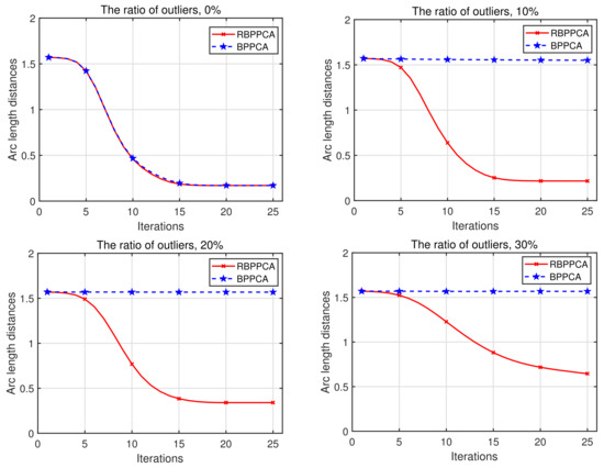
In this test, we start with $C^{(0)}=rand(d_c,q_c)$, $R^{(0)}=rand(d_r,q_r)$, ${\sigma }_c^{(0)}=1$, ${\sigma }_r^{(0)}=1$ and ${\nu }^{(0)}=1$, then consider the effect of the ratio of outliers, i.e., $N_o/N$, which is varied from 0 to 30% with a stride length of 10% in this example. In these cases, the estimated values of $\nu$ are all $\nu =1$. If we use other initial values ${\nu }^{(0)}$ here, the computed $\nu$ also converges to one as iterations increase. The corresponding numerical results of arc length distances are plotted in Figure 1. Figure 1 shows that the RBPPCA and BPPCA methods almost perform with the same convergence behavior when the data matrices are without outliers.

Figure 1. Convergence behaviors of RBPPCA and BPPCA with the ratio of outliers being 0%, 10%, 20% and 30%, respectively.

As the ratio of outliers goes to 30%, it is reasonable that more iterations are required for the RBPPCA method to achieve a satisfactory accuracy. Unlike the BPPCA method, the presented RBPPCA method is more robust to outliers because the arc length distances of the BPPCA method are always held to approximately $1.5$ when the data includes outliers.

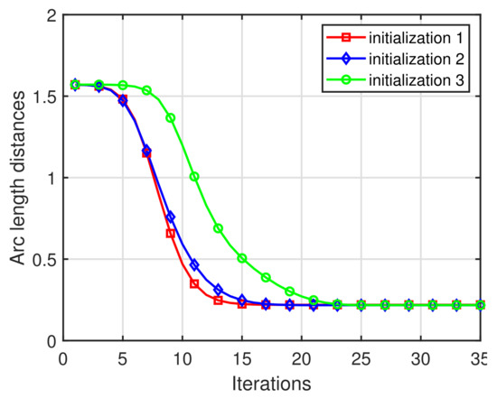
In this example, we also test the impact of the initializations on $C^{(0)}$ and $R^{(0)}$, and the sample size N, respectively, based on the synthetic data having 10% outliers. Three different types of initializations of $C^{(0)}$ and $R^{(0)}$ are set as follows:

(1)

initialization 1: $C^{(0)}=rand(d_c,q_c)$ and $R^{(0)}=rand(d_r,q_r)$;

(2)

initialization 2: $C^{(0)}=randn(d_c,q_c)$ and $R^{(0)}=randn(d_r,q_r)$;

(3)

initialization 3:

$$C^{(0)}=R^{(0)}=\left[\begin{array}{cccccccc}1& 0& 0& 0& 0& 0& 0& 0\\ 0& 1& 0& 0& 0& 0& 0& 0\\ ⋮& ⋮& ⋮& ⋮& ⋮& ⋮& ⋮& ⋮\\ 0& 0& 0& 0& 0& 0& 0& 1\\ \frac{9}{d_c}& \frac{9}{d_c}+9& sin(9)& cos(9)& tan(9)& cot(9)& sec(9)& csc(9)\\ ⋮& ⋮& ⋮& ⋮& ⋮& ⋮& ⋮& ⋮\\ \frac{d_c}{d_c}& \frac{d_c}{d_c}+d_c& sin(d_c)& cos(d_c)& tan(d_c)& cot(d_c)& sec(d_c)& csc(d_c)\end{array}\right],$$

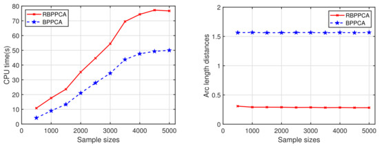
and other parameters are fixed to be the same. The results associated with the different initializations are shown in Figure 2. Inspection of the plot illustrates that our RBPPCA method appears to be insensitive to different initializations, since the convergence behaviors of the RBPPCA method based on different initializations do not have a significant difference. Figure 3 presents the required CPU time in seconds and the quantities of arc length distances of the BPPCA and RBPPCA methods with the number of iterations being 25 with respect to the number of samples, where the sample size N varies from 200 to 5000 with a stride length of 200. Such graphs covey the fact that with the increase of the sample size N, the BPPCA and RBPPCA methods both required more CPU time for 25 iterations, and the BPPCA method needs less time complexity than RBPPCA as we stated in the remarks of Algorithm 1. However, the bigger N does not lead to the improved arc length distances of the BPPCA method.

Figure 2. Convergence behaviors of RBPPCA for three different types of initialization.

Figure 3. CPU time in seconds (left) and arc length distances (right) of BPPCA and RBPPCA with the number of iterations being 25 with the sample size N from 200 to 5000.

Example 2

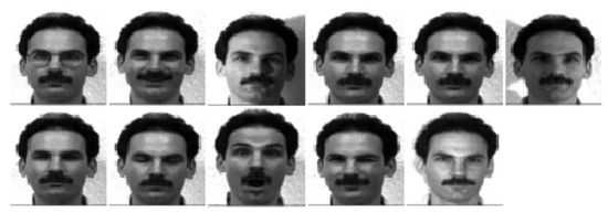
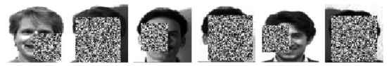
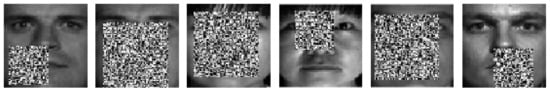
(Experiments on face image databases).In this example, all of the experiments are based on two publicly available face image databases: the Yale face database ( Available from http://vision.ucsd.edu/content/yale-face-database) (accessed on 22 September 2021), and the Yale B face database (Available from http://vision.ucsd.edu/~leekc/ExtYaleDatabase/ExtYaleB.html) (accessed on 22 September 2021).The Yale face database includes different face orientations, facial expression, and whether there exist glasses, and the Yale B face database is collected under different illumination conditions. We select 265 face images of 15 individuals for each database. Each person has 11 images, and these images are cropped to $64\times 64$ pixels. For each individual, eight images are randomly selected as the training set, and the rest are the test set. Then, we randomly select two and four images from the eight images in the training set to be corrupted as outliers, respectively. Half of the corrupted images are generated by replacing part of the original image with a $30\times 30$ rectangle of noise, and the other half of corrupted images use a $50\times 50$ rectangle of noise to replace it. Within each rectangle, the pixel value comes from a uniform distribution on the interval $[0,255]$. Then, we rescale the images from the range of [0, 255] to the range [0, 1]. Some original and corrupted images of the Yale and Yale B databases are shown in Figure 4, Figure 5, Figure 6 and Figure 7, respectively. The iteration of BPPCA and RBPPCA is stopped when their corresponding relative changes of the log-likelihood defined in (29) are smaller than ${10}^{-5}$.

Figure 4. One set of processed samples from the Yale face database.

Figure 5. Some generated outlier face images in the training set from the Yale face database.

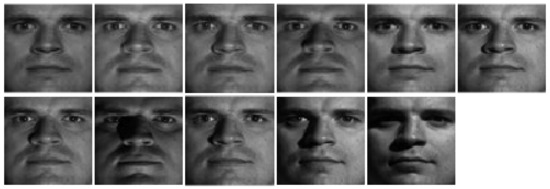
Figure 6. Eleven images of an individual from the Yale B face database.

Figure 7. Some corrupted face images in the training set of the Yale B face database.

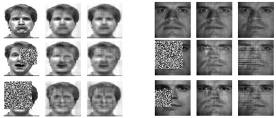
We run the BPPCA and RBBPCA algorithms for the original data set and the corrupted data set, respectively, with the order of Z in (11) being $q_c=q_r=8$, and consider the reconstructed images ${\widehat{X}}_n$ defined in (30) based on the computed results. A comparison of the reconstructed images based on the original data set and corrupted data set with two corrupted images for each individual is shown in Figure 8. In Figure 8, the first, second and third columns are the original images, the reconstructed images of RBPPCA, and the reconstructed images of BPPCA for the Yale (left) and Yale B (right) databases, respectively, and the images of the first, second and third rows are shown based on the original, corrupted data sets with $30\times 30$ rectangles of noise, and corrupted data sets with $50\times 50$ rectangles of noise, respectively. The BPPCA and RBPPCA almost perform the same as the reconstructed images on the original data set. However, for corrupted data sets, the reconstructed performance of RBPPCA presents better images than BPPCA because it tries to explain noise information.

Figure 8. Original images (the first column), reconstructed images by RBPPCA (the second column), and reconstructed images by BPPCA (the third column) of the Yale (left) and Yale B (right) databases, respectively.

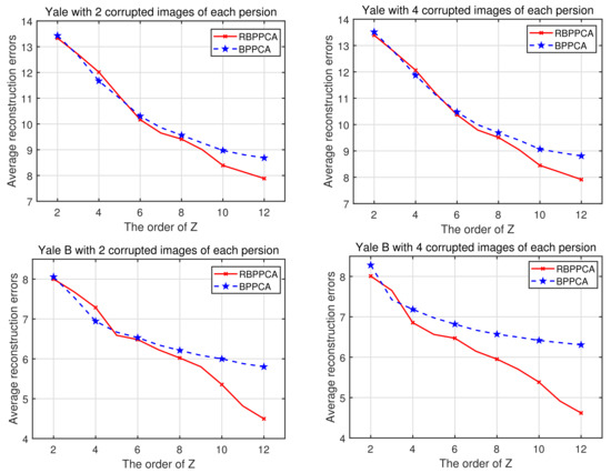
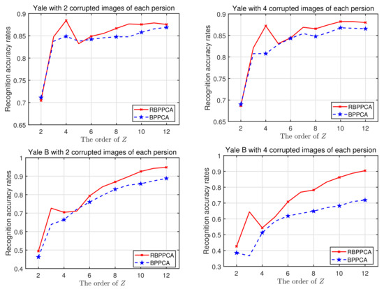
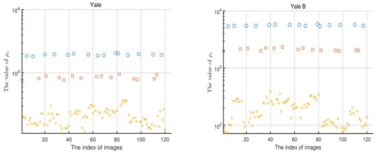
We also compare the average reconstruction errors $\eta ={\sum }_{n=1}^N{\parallel X_n-{\widehat{X}}_n\parallel }_F/N$ and the recognition accuracy rates for the RBPPCA and BPPCA algorithms in the cases where each person has two corrupted images and four corrupted images, respectively, where recognition accuracy rates are calculated based on the nearest neighbor classifier (1-NN) which is employed for the classification. The average reconstruction errors and recognition accuracy rates versus the order of Z are plotted in Figure 9 and Figure 10, respectively. As expected, the average reconstruction errors decrease, while the recognition accuracy rates rise as the order of Z increases. In these cases, our proposed RBPPCA algorithm outperforms the BPPCA algorithm in reducing average reconstruction errors and enhancing the recognition accuracy. In addition, another advantage of robust probabilistic algorithms based on t distributions is outlier detection. By [14], we can compute ${\rho }_n={\left[vec(X_n-M)\right]}^T{({\Sigma }_r\otimes {\Sigma }_c)}^{-1}vec(X_n-M)$ as the standard of outlier detection. Figure 11 is the scatter chart for ${\rho }_n$ of all the images in the training set of the Yale and Yale B databases with two corrupted images for one person, respectively. It is exhibited that the quantity of ${\rho }_n$ can be divided into three parts. Notice that these three parts correspond to the images with no noise, a $30\times 30$ rectangle of noise, and a $50\times 50$ rectangle of noise, respectively. Hence, the comparison of ${\rho }_n$ provides a method for judging the outliers.

Figure 9. Average reconstruction errors of the BPPCA and RBPPCA algorithms vs. the order of Z for the Yale and Yale B databases with 2 and 4 corrupted images of each individual, respectively.

Figure 10. Recognition accuracy rates of the BPPCA and RBPPCA algorithms vs. the order of Z for the Yale and Yale B databases with 2 and 4 corrupted images of each individual, respectively.

Figure 11. ${\rho }_n$ of each image in the Yale (left) and Yale B (right) databases, respectively, with 2 corrupted images of each individual.

Example 3

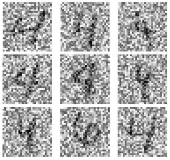
(Experiments on the MNIST dataset).In Example 2, it is shown that RBPPCA is superior to BPPCA when the data sets contain outliers. In this example, we compare the RBPPCA algorithm to the tPPCA [14] and L1-PPCA [15] algorithms based on handwritten digit images from the MNIST (Available from http://yann.lecun.com/exdb/mnist) (accessed on 22 September 2021) database in which each image has $28\times 28$ pixels. We choose 59 images of the digit 4 as the training data set, and randomly select nine of them to be corrupted as outliers. The way of corrupting the images is to add noise from a uniform distribution on the interval$[0,510]$, and then normalize all images to the range$[0,1]$. The normalized corrupted images of the digit 4 are shown in Figure 12. The RBPPCA, tPPCA [14] and L1-PPCA [15] algorithms are implemented with 100 iterations for the original data set of the digit 4 and the corrupted data set, respectively.

Figure 12. The normalized corrupted images of the digit 4.

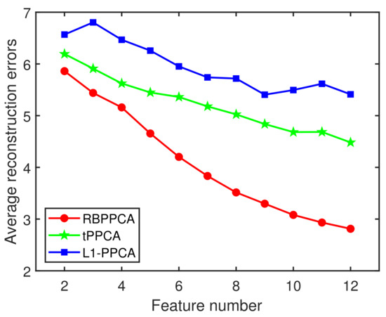
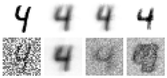
Figure 13 presents the average reconstruction errors of the RBBPCA, tPPCA and L1-PPCA algorithms where the feature number is the order of Z for the RBBPCA algorithm and is the dimension of the low-dimensional representation for the tPPCA and L1-PPCA algorithms. It is observed that the performance of our RBPPCA algorithm is superior to other algorithms. The reconstructed behaviors of different algorithms based on the original data set of the digit 4 and the corrupted data set with $q_c=q_r=1$ are shown in Figure 14. In Figure 14, the first column is the original images, and the second, third and fourth columns are the reconstructed images by the RBBPCA, tPPCA and L1-PPCA algorithms, respectively. As shown in Figure 14, compared to the tPPCA and L1-PPCA algorithms, the RBPPCA algorithm performs better reconstruction outcomes in such a case.

Figure 13. Average reconstruction errors of the RBPPCA, tPPCA and L1-PPCA algorithms vs. feature number on the MINST database.

Figure 14. Original images of the digit 4 (the first column), images reconstructed by RBPPCA (the second column), images reconstructed by tPPCA (the third column), and images reconstructed by L1-PPCA (the fourth column). The images shown in the first and second rows are based on the original and corrupted image data sets, respectively.

5. Conclusions

To remedy the problem that data are assumed to follow a matrix variate Gaussian distribution which is sensitive to outliers, in this paper, we proposed a robust BPPCA algorithm (RBPPCA), i.e., Algorithm 1, by replacing the matrix variate Gaussian distribution with the matrix variate t distribution for noise. Compared to BPPCA, owing to the matrix variate t distribution having a significantly heavy tail property, our proposed RBPPCA method combined with AECM for estimating parameters can deal with 2-D data sets in the presence of outliers. The numerical examples based on a synthetic and two publicly available real data sets, Yale and Yale B, are presented to state that Algorithm 1 is far superior to the BPPCA algorithm in computational accuracy, reconstruction performance, average reconstruction errors, recognition accuracy rates, and outlier detection. It is also shown by numerical examples based on the MNIST database that our RBPPCA method outperforms the tPPCA and L1-PPCA algorithms.

References

- Bishop, C.M. Pattern Recognition and Machine Learning; Springer: Berlin/Heidelberg, Germany, 2006. [Google Scholar]
- Burges, C.J.C. Dimension Reduction: A Guided Tour; Now Publishers Inc.: Noord-Brabant, The Netherlands, 2010. [Google Scholar]
- Ma, Y.; Zhu, L. A review on dimension reduction. Int. Stat. Rev. 2013, 81, 134–150. [Google Scholar]
- Jolliffe, I.T. Principal Component Analysis; Springer: Berlin/Heidelberg, Germany, 2002. [Google Scholar]
- Yang, J.; Zhang, D.; Frangi, A.F.; Yang, J. Two-dimensional PCA: A new approach to appearance-based face representation and recognition. IEEE Trans. Pattern Anal. Mach. Intell. 2004, 26, 131–137. [Google Scholar]
- Ye, J. Generalized low rank approximations of matrices. Mach. Learn. 2005, 61, 167–191. [Google Scholar]
- Zhang, D.; Zhou, Z.H. (2D) 2PCA: Two-directional two-dimensional PCA for efficient face representation and recognition. Neurocomputing 2005, 69, 224–231. [Google Scholar]
- Tipping, M.E.; Bishop, C.M. Probabilistic principal component analysis. J. R. Stat. Soc. Ser. B Stat. Methodol. 1999, 61, 611–622. [Google Scholar]
- Murphy, K.P. Machine Learning: A Probabilistic Perspective; MIT Press: Cambridge, MA, USA, 2012. [Google Scholar]
- Yu, S.; Bi, J.; Ye, J. Matrix-variate and higher-order probabilistic projections. Data Min. Knowl. Discov. 2011, 22, 372–392. [Google Scholar]
- Gupta, A.K.; Nagar, D.K. Matrix Variate Distributions; CRC Press: Boca Raton, FL, USA, 2018; Volume 104. [Google Scholar]
- Zhao, J.; Philip, L.H.; Kwok, J.T. Bilinear probabilistic principal component analysis. IEEE Trans. Neural Netw. Learn. Syst. 2012, 23, 492–503. [Google Scholar]
- Zhao, J.; Jiang, Q. Probabilistic PCA for t distributions. Neurocomputing 2006, 69, 2217–2226. [Google Scholar]
- Chen, T.; Martin, E.; Montague, G. Robust probabilistic PCA with missing data and contribution analysis for outlier detection. Comput. Stat. Data Anal. 2009, 53, 3706–3716. [Google Scholar]
- Gao, J. Robust L1 principal component analysis and its Bayesian variational inference. Neural Comput. 2008, 20, 555–572. [Google Scholar] [CrossRef] [PubMed]
- Ju, F.; Sun, Y.; Gao, J.; Hu, Y.; Yin, B. Image outlier detection and feature extraction via L1-norm-based 2D probabilistic PCA. IEEE Trans. Image Process. 2015, 24, 4834–4846. [Google Scholar] [CrossRef] [PubMed]
- Galimberti, G.; Soffritti, G. A multivariate linear regression analysis using finite mixtures of t distributions. Comput. Stat. Data Anal. 2014, 71, 138–150. [Google Scholar] [CrossRef]
- Morris, K.; McNicholas, P.D.; Scrucca, L. Dimension reduction for model-based clustering via mixtures of multivariate t-distributions. Adv. Data Anal. Classif. 2013, 7, 321–338. [Google Scholar] [CrossRef]
- Pesevski, A.; Franczak, B.C.; McNicholas, P.D. Subspace clustering with the multivariate-t distribution. Pattern Recognit. Lett. 2018, 112, 297–302. [Google Scholar] [CrossRef] [Green Version]
- Teklehaymanot, F.K.; Muma, M.; Zoubir, A.M. Robust Bayesian cluster enumeration based on the t distribution. Signal Process. 2021, 182, 107870. [Google Scholar] [CrossRef]
- Wei, X.; Yang, Z. The infinite Student’s t-factor mixture analyzer for robust clustering and classification. Pattern Recognit. 2012, 45, 4346–4357. [Google Scholar] [CrossRef]
- Zhou, X.; Tan, C. Maximum likelihood estimation of Tobit factor analysis for multivariate t-distribution. Commun. Stat. Simul. Comput. 2009, 39, 1–16. [Google Scholar] [CrossRef]
- Lange, K.L.; Little, R.J.A.; Taylor, J.M.G. Robust statistical modeling using the t distribution. J. Am. Stat. Assoc. 1989, 84, 881–896. [Google Scholar] [CrossRef] [Green Version]
- Meng, X.L.; Van Dyk, D. The EM algorithm—An old folk-song sung to a fast new tune. J. R. Stat. Soc. Ser. B Stat. Methodol. 1997, 59, 511–567. [Google Scholar] [CrossRef]
- Zhou, Y.; Lu, H.; Cheung, Y. Bilinear probabilistic canonical correlation analysis via hybrid concatenations. In Proceedings of the AAAI Conference on Artificial Intelligence, San Francisco, CA, USA, 5–9 October 2017; Volume 31. [Google Scholar]
- Coleman, T.; Branch, M.A.; Grace, A. Optimization toolbox. In For Use with MATLAB. User’s Guide for MATLAB 5, Version 2, Relaese II; 1999; Available online: https://www.dpipe.tsukuba.ac.jp/~naito/optim_tb.pdf (accessed on 20 September 2021).
- Schrage, L. LINGO User’s Guide; LINDO System Inc.: Chicago, IL, USA, 2006. [Google Scholar]
- Stewart, G.W. Matrix Algorithms: Volume II: Eigensystems; SIAM: Philadelphia, PA, USA, 2001. [Google Scholar]
Publisher’s Note: MDPI stays neutral with regard to jurisdictional claims in published maps and institutional affiliations. |
© 2021 by the authors. Licensee MDPI, Basel, Switzerland. This article is an open access article distributed under the terms and conditions of the Creative Commons Attribution (CC BY) license (https://creativecommons.org/licenses/by/4.0/).