
Metaheuristics for a Flow Shop Scheduling Problem with Urgent Jobs and Limited Waiting Times


Abstract
1. Introduction
2. Previous Studies
3. Problem Description and an MIP Model
- no job can be preempted;
- machines do not fail (no breakdown);
- all normal jobs are available to be processed at time zero (beginning of the scheduling horizon);
- release times and arriving times of urgent jobs are positive and given in advance;
- the due date of an urgent job i is set to the earliest possible completion time assuming that the urgent job i is started immediately as arrived at the flow shop and processed without waiting, i.e., di = ri + pi1 + pi2.
4. Heuristic Algorithms
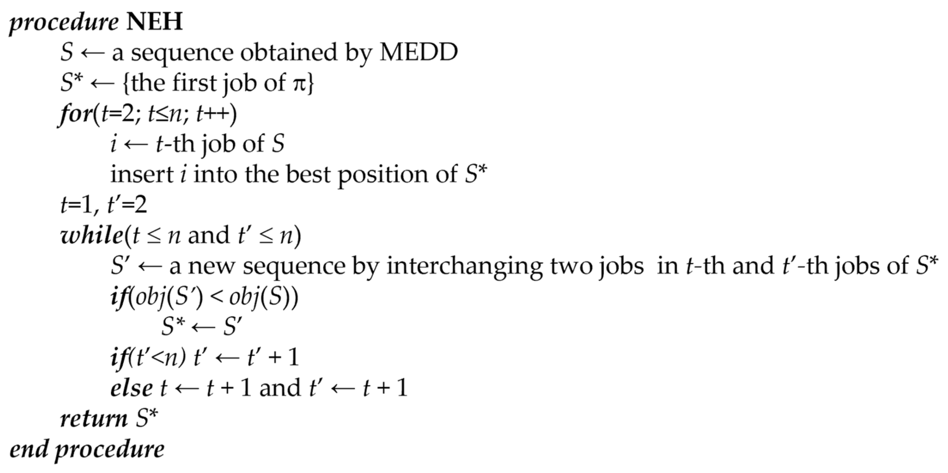
4.1. Initial Seed Sequence
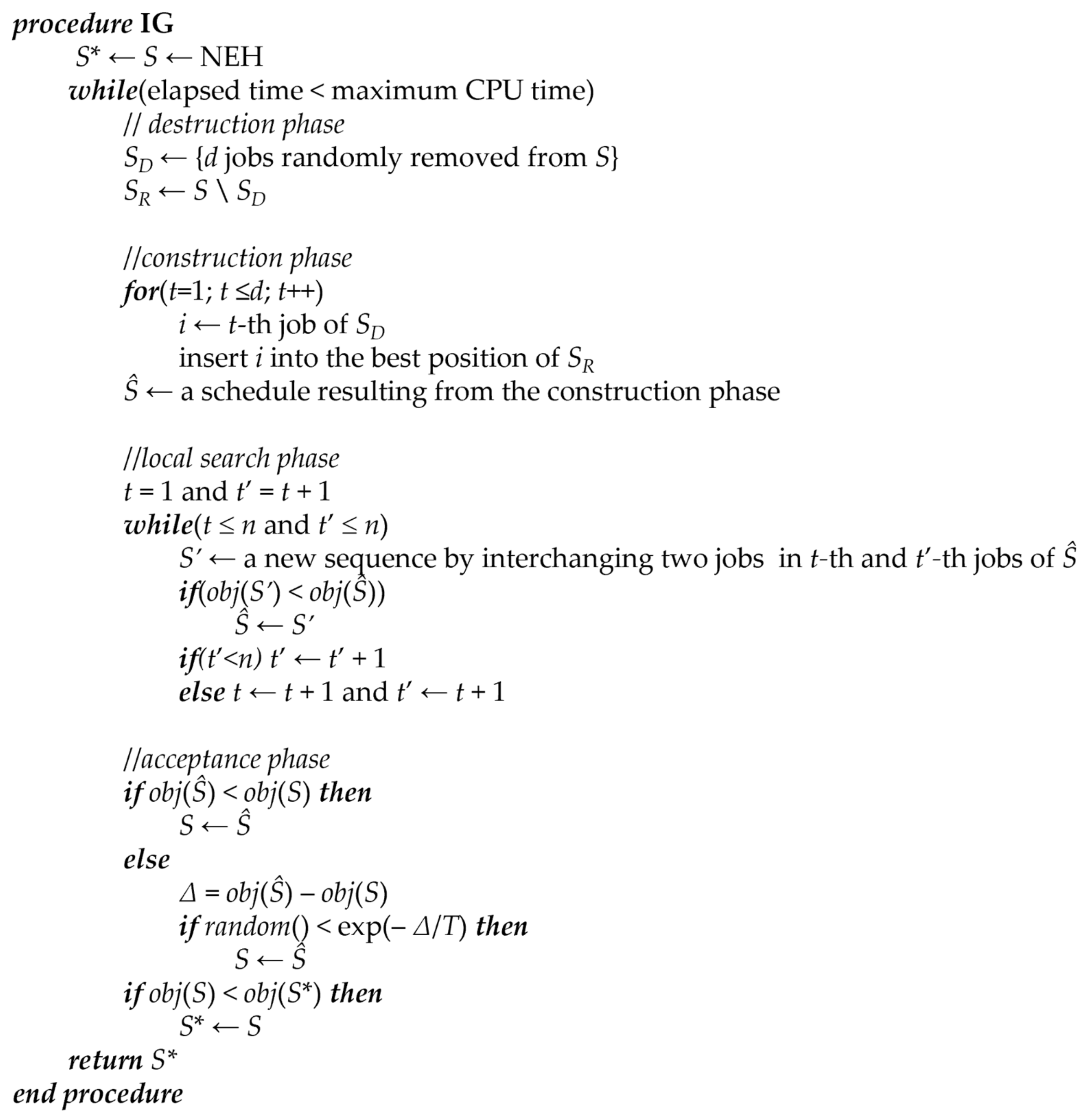
4.2. Iterated Greedy Algorithm
- In the proposed IG, d jobs are removed randomly from a current solution (S) in the destruction phase. Then, two partial schedules are generated. One (SD) is a schedule consisting of d jobs removed from S, the other is a partial schedule (SR) with (n − d) jobs. After that, in the construction phase, a complete schedule is constructed by inserting the jobs of SD into the best positions of SR, such as the for-loop in Figure 1. After these two phases, the complete schedule is improved by a local search procedure. In this IG, the interchange method used in NEH is implemented for the improvement. Completing the local search, the new schedule (S’) is compared to the current schedule (S). If S’ is better than S, i.e., obj(S’) < obj(S), S’ replaces S. Otherwise, borrowing the concept of an acceptance in a simulated annealing algorithm, the replacement is accepted with a probability exp(– Δ/T), where Δ = obj(S’) – obj(S), and T is an adjustable parameter (called temperature) in the IG. However, unlike SA, T is constant in IG. The temperature value T is calculated assuggested in [44] for the permutation flow shop scheduling problem. In this study, m = 2. These four phases are repeated until a termination condition is satisfied. Herein, the maximum computation time is used for the termination condition. The whole procedure of IG is summarized in Figure 2. In the procedure, let random() denote a function to return a random number greater than or equal to zero and less than one.
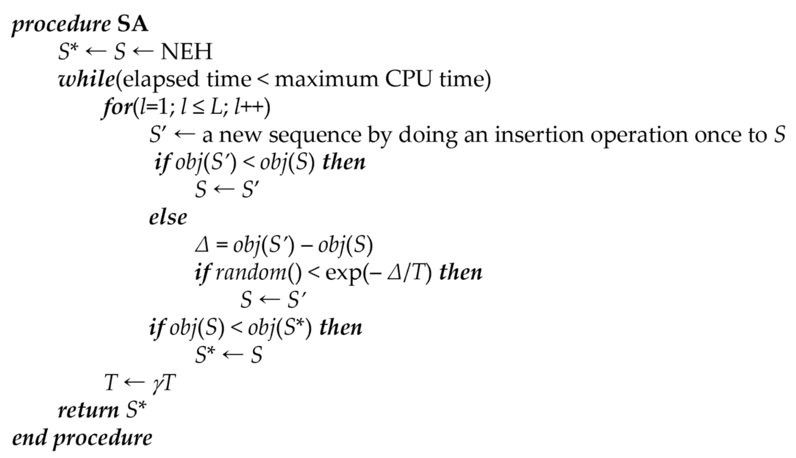
4.3. Simulated Annealing Algorithm
5. Computational Experiments
6. Discussion and Conclusions
Author Contributions
Funding
Data Availability Statement
Conflicts of Interest
References
- Jeong, B.; Shim, S.O. Heuristic algorithms for two-machine re-entrant flowshop scheduling problem with jobs of two classes. J. Adv. Mech. Des. Syst. Manuf. 2017, 11, 5. [Google Scholar] [CrossRef][Green Version]
- Wang, B.L.; Huang, K.; Li, T.K. Permutation flowshop scheduling with time lag constraints and makespan criterion. Comput. Ind. Eng. 2018, 120, 1–14. [Google Scholar] [CrossRef]
- An, Y.J.; Kim, Y.D.; Choi, S.W. Minimizing makespan in a two-machine flowshop with a limited waiting time constraint and sequence-dependent setup times. Comput. Oper. Res. 2016, 71, 127–136. [Google Scholar] [CrossRef]
- Koulamas, C. The Total Tardiness Problem: Review and Extensions. Oper. Res. 1994, 42, 1025–1041. [Google Scholar] [CrossRef]
- Yang, D.-L.; Maw-Sheng, C. A two-machine flowshop sequencing problem with limited waiting time constraints. Comput. Ind. Eng. 1995, 28, 8. [Google Scholar] [CrossRef]
- Liang, J.; Wang, P.; Guo, L.; Qu, B.; Yue, C.; Yu, K.; Wang, Y. Multi-objective flow shop scheduling with limited buffers using hybrid self-adaptive differential evolution. Memetic. Comput. 2019, 11, 407–422. [Google Scholar] [CrossRef]
- Anjana, V.; Sridharan, R.; Ram Kumar, P.N. Metaheuristics for solving a multi-objective flow shop scheduling problem with sequence-dependent setup times. J. Sched. 2020, 23, 49–69. [Google Scholar] [CrossRef]
- Rifai, A.P.; Mara, S.T.W.; Sudiarso, A. Multi-objective distributed reentrant permutation flow shop scheduling with sequence-dependent setup time. Expert Syst. Appl. 2021, 183, 115339. [Google Scholar] [CrossRef]
- Zhang, B.; Pan, Q.-k.; Gao, L.; Li, X.-y.; Meng, L.-l.; Peng, K.-k. A multiobjective evolutionary algorithm based on decomposition for hybrid flowshop green scheduling problem. Comput. Ind. Eng. 2019, 136, 325–344. [Google Scholar] [CrossRef]
- Han, Y.; Li, J.; Sang, H.; Liu, Y.; Gao, K.; Pan, Q.-K. Discrete evolutionary multi-objective optimization for energy-efficient blocking flow shop scheduling with setup time. Appl. Soft. Comput. 2020, 93, 106343. [Google Scholar] [CrossRef]
- Lu, C.; Gao, L.; Yi, J.; Li, X. Energy-efficient scheduling of distributed flow shop with heterogeneous factories: A real-world case from automobile industry in China. IEEE Trans. Ind. Inform. 2021, 17, 6687–6696. [Google Scholar] [CrossRef]
- Agnetis, A.; Mirchandani, P.B.; Pacciarelli, D.; Pacifici, A. Scheduling problems with two competing agents. Oper. Res. 2004, 52, 229–242. [Google Scholar] [CrossRef]
- Baker, K.R.; Cole Smith, J. A multiple-criterion model for machine scheduling. J. Sched. 2003, 6, 7–16. [Google Scholar] [CrossRef]
- Ng, C.T.; Cheng, T.C.E.; Yuan, J.J. A note on the complexity of the problem of two-agent scheduling on a single machine. J. Comb. Optim. 2006, 12, 387–394. [Google Scholar] [CrossRef]
- Leung, J.Y.-T.; Pinedo, M.; Wan, G. Competitive two-agent scheduling and its applications. Oper. Res. 2010, 58, 458–469. [Google Scholar] [CrossRef]
- Cheng, T.C.E.; Ng, C.T.; Yuan, J.J. Multi-agent scheduling on a single machine to minimize total weighted number of tardy jobs. Theor. Comput. Sci. 2006, 362, 273–281. [Google Scholar] [CrossRef]
- Cheng, T.C.E.; Ng, C.T.; Yuan, J.J. Multi-agent scheduling on a single machine with max-form criteria. Eur. J. Oper. Res. 2008, 188, 603–609. [Google Scholar] [CrossRef]
- Liu, P.; Tang, L. Two-Agent Scheduling with Linear Deteriorating Jobs on a Single Machine; Springer: Berlin/Heidelberg, Germany, 2008; pp. 642–650. [Google Scholar]
- Lee, W.C.; Chung, Y.H.; Huang, Z.R. A single-machine bi-criterion scheduling problem with two agents. Appl. Math. Comput. 2013, 219, 10831–10841. [Google Scholar] [CrossRef]
- Wan, L.; Yuan, J.J.; Wei, L.J. Pareto optimization scheduling with two competing agents to minimize the number of tardy jobs and the maximum cost. Appl. Math. Comput. 2016, 273, 912–923. [Google Scholar] [CrossRef]
- Lee, W.C.; Chen, S.K.; Wu, C.C. Branch-and-bound and simulated annealing algorithms for a two-agent scheduling problem. Expert Syst. Appl. 2010, 37, 6594–6601. [Google Scholar] [CrossRef]
- Lee, W.C.; Chen, S.K.; Chen, C.W.; Wu, C.C. A two-machine flowshop problem with two agents. Comput. Oper. Res. 2011, 38, 98–104. [Google Scholar] [CrossRef]
- Mor, B.; Mosheiov, G. Polynomial time solutions for scheduling problems on a proportionate flowshop with two competing agents. J. Oper. Res. Soc. 2014, 65, 151–157. [Google Scholar] [CrossRef]
- Fan, B.Q.; Cheng, T.C.E. Two-agent scheduling in a flowshop. Eur. J. Oper. Res. 2016, 252, 376–384. [Google Scholar] [CrossRef]
- Jeong, B.; Kim, Y.D.; Shim, S.O. Algorithms for a two-machine flowshop problem with jobs of two classes. Int. Trans. Oper. Res. 2020, 27, 3123–3143. [Google Scholar] [CrossRef]
- Azerine, A.; Boudhar, M.; Rebaine, D. A two-machine no-wait flow shop problem with two competing agents. J. Comb. Optim. 2021, in press. [Google Scholar] [CrossRef]
- Bouquard, J.-L.; Lenté, C. Two-machine flow shop scheduling problems with minimal and maximal delays. 4OR 2006, 4, 15–28. [Google Scholar] [CrossRef]
- Joo, B.J.; Kim, Y.D. A branch-and-bound algorithm for a two-machine flowshop scheduling problem with limited waiting time constraints. J. Oper. Res. Soc. 2009, 60, 572–582. [Google Scholar] [CrossRef]
- Hamdi, I.; Loukil, T. Minimizing total tardiness in the permutation flowshop scheduling problem with minimal and maximal time lags. Oper. Res. Ger. 2015, 15, 95–114. [Google Scholar] [CrossRef]
- Dhouib, E.; Teghem, J.; Loukil, T. Lexicographic optimization of a permutation flow shop scheduling problem with time lag constraints. Int. Trans. Oper. Res. 2013, 20, 213–232. [Google Scholar] [CrossRef]
- Kim, H.J.; Lee, J.H. Three-machine flow shop scheduling with overlapping waiting time constraints. Comput. Oper. Res. 2019, 101, 93–102. [Google Scholar] [CrossRef]
- Lee, J.Y. A genetic algorithm for a two-machine flowshop with a limited waiting time constraint and sequence-dependent setup times. Math. Probl. Eng. 2020, 2020, 8833645. [Google Scholar] [CrossRef]
- Yu, T.S.; Kim, H.J.; Lee, T.E. Minimization of waiting time variation in a generalized two-machine flowshop with waiting time constraints and skipping jobs. IEEE T Semicond. Manuf. 2017, 30, 155–165. [Google Scholar] [CrossRef]
- Li, Y.; Dai, Z. A two-stage flow-shop scheduling problem with incompatible job families and limited waiting time. Eng. Optim. 2020, 52, 484–506. [Google Scholar] [CrossRef]
- Hamdi, I.; Toumi, S. MILP models and valid inequalities for the two-machine permutation flowshop scheduling problem with minimal time lags. J. Ind. Eng. Int. 2019, 15, 223–229. [Google Scholar] [CrossRef][Green Version]
- Lima, A.; Borodin, V.; Dauzère-Pérès, S.; Vialletelle, P. Sampling-based release control of multiple lots in time constraint tunnels. Comput. Ind. 2019, 110, 3–11. [Google Scholar] [CrossRef]
- Lima, A.; Borodin, V.; Dauzère-Pérès, S.; Vialletelle, P. A sampling-based approach for managing lot release in time constraint tunnels in semiconductor manufacturing. Int. J. Prod. Res. 2021, 59, 860–884. [Google Scholar] [CrossRef]
- Maassena, K.; Perez-Gonzalez, P.; Gunther, L.C. Relationship between common objective functions, idle time and waiting time in permutation flow shop scheduling. Comput. Oper. Res. 2020, 121, 104965. [Google Scholar] [CrossRef]
- Samarghandi, H. Minimizing the makespan in a flow shop environment under minimum and maximum time-lag constraints. Comput. Ind. Eng. 2019, 136, 614–634. [Google Scholar] [CrossRef]
- Ye, S.; Zhao, N.; Li, K.D.; Lei, C.J. Efficient heuristic for solving non-permutation flow-shop scheduling problems with maximal and minimal time lags. Comput. Ind. Eng. 2017, 113, 160–184. [Google Scholar] [CrossRef]
- Zhou, N.; Wu, M.; Zhou, J. Research on power battery formation production scheduling problem with limited waiting time constraints. In Proceedings of the 2018 10th International Conference on Communication Software and Networks, Chengdu, China, 6–9 July 2018; pp. 497–501. [Google Scholar]
- Nawaz, M.; Enscore, E.E.; Ham, I. A heuristic algorithm for the m-machine, n-job flow-shop sequencing problem. Omega 1983, 11, 91–95. [Google Scholar] [CrossRef]
- Ruiz, R.; Stutzle, T. A simple and effective iterated greedy algorithm for the permutation flowshop scheduling problem. Eur. J. Oper. Res. 2007, 177, 2033–2049. [Google Scholar] [CrossRef]
- Osman, I.H.; Potts, C.N. Simulated annealing for permutation flow-shop scheduling. Omega 1989, 17, 551–557. [Google Scholar] [CrossRef]
- Johnson, S.M. Optimal two- and three-stage production schedules with setup times included. Nav. Res. Logist. Q. 1954, 1, 61–68. [Google Scholar] [CrossRef]


| Symbol | Definition |
|---|---|
| i | index for jobs (i = 1, 2, …, n) |
| k | index for machines (k = 1, 2) |
| t | index for positions in a sequence |
| [t] | index of the job in the tth position in a sequence |
| pik | processing time of job i on machine k |
| ri | release time of job i (=0 if job i is a normal job) |
| wi | limited waiting time of job i |
| di | due date of job i (=ri + pi for i ∈ JA, and a large number for i ∈ JB) |
| yi | =1 if job i is a normal job, and 0 otherwise |
| xit | =1 if job i is placed in the tth position in a sequence, and 0 otherwise |
| ctk | completion time of the tth position on machine k |
| ci | completion time of job i on machine 2 |
| τi | tardiness of job i |
| Z | the makespan of normal jobs |
| α | weight for total tardiness of urgent jobs (0 ≤ α ≤ 1) |
| 1 − α | weight for the makespan of normal jobs |
| M | a large number |
| S | (partial or complete) schedule |
| Si | a schedule in which job i is added to the end of S |
| C(S) | completion time of S |
| UA (UB) | set of urgent (normal) jobs not scheduled yet |
| obj(S) | objective function value of S |
| n | h | α | ||
|---|---|---|---|---|
| 0.5 | 0.7 | 0.9 | ||
| 10 | 0.3 | 0.93, (0) 1 | 0.85 (0) | 0.54 (0) |
| 0.5 | 1.37 (0) | 1.23 (0) | 1.03 (0) | |
| 0.7 | 2.62 (0) | 2.48 (0) | 2.1 (0) | |
| 20 | 0.3 | 2225.24 (1) | 659.25 (0) | 341.35 (0) |
| 0.5 | 3600 (5) | 3145.93 (4) | 2751.78 (3) | |
| 0.7 | 3600 (5) | 3600 (5) | 3600 (5) | |
| 30 | 0.3 | 3600 (5) | 3600 (5) | 3600 (5) |
| 0.5 | 3600 (5) | 3600 (5) | 3600 (5) | |
| 0.7 | 3600 (5) | 3600 (5) | 3600 (5) |
| Algorithm | n = 10 | 20 | 30 |
|---|---|---|---|
| MEDD | 1.048 (0) 1 | 1.371 (0) | 2.711 (0) |
| NEH | 0.096 (4) | 0.158 (0) | 0.266 (0) |
| IG(50) | 0.003 (21) | −0.001 (20) | −0.007 (29) |
| IG(100) | 0.003 (21) | −0.001 (20) | −0.008 (30) |
| SA(50) | 0.006 (19) | 0.002 (16) | −0.001 (27) |
| SA(100) | 0.006 (19) | 0.002 (16) | −0.001 (27) |
| n | h | α | IG(50) | IG(100) | SA(50) | SA(100) | TS(50) | TS(100) |
|---|---|---|---|---|---|---|---|---|
| 50 | 0.3 | 0.5 | 0.0010 | 0.0003 | 0.0029 | 0.0026 | 0.0220 | 0.0201 |
| 0.7 | 0.0007 | 0.0000 | 0.0048 | 0.0045 | 0.0327 | 0.0304 | ||
| 0.9 | 0.0010 | 0.0007 | 0.0046 | 0.0041 | 0.0233 | 0.0195 | ||
| 0.5 | 0.5 | 0.0011 | 0.0000 | 0.0071 | 0.0068 | 0.0242 | 0.0200 | |
| 0.7 | 0.0050 | 0.0034 | 0.0128 | 0.0128 | 0.0113 | 0.0084 | ||
| 0.9 | 0.0067 | 0.0028 | 0.0174 | 0.0169 | 0.0047 | 0.0018 | ||
| 0.7 | 0.5 | 0.0048 | 0.0029 | 0.0067 | 0.0061 | 0.0071 | 0.0042 | |
| 0.7 | 0.0016 | 0.0005 | 0.0166 | 0.0163 | 0.0052 | 0.0028 | ||
| 0.9 | 0.0030 | 0.0011 | 0.0082 | 0.0075 | 0.0123 | 0.0094 | ||
| 100 | 0.3 | 0.5 | 0.0021 | 0.0010 | 0.0030 | 0.0023 | 0.0608 | 0.0574 |
| 0.7 | 0.0037 | 0.0027 | 0.0042 | 0.0035 | 0.0695 | 0.0561 | ||
| 0.9 | 0.0002 | 0.0000 | 0.0047 | 0.0038 | 0.0916 | 0.0608 | ||
| 0.5 | 0.5 | 0.0062 | 0.0010 | 0.0204 | 0.0183 | 0.0856 | 0.0703 | |
| 0.7 | 0.0150 | 0.0103 | 0.0158 | 0.0151 | 0.0777 | 0.0675 | ||
| 0.9 | 0.0325 | 0.0276 | 0.0335 | 0.0183 | 0.0989 | 0.0759 | ||
| 0.7 | 0.5 | 0.0034 | 0.0020 | 0.0136 | 0.0119 | 0.0212 | 0.0171 | |
| 0.7 | 0.0100 | 0.0060 | 0.0154 | 0.0128 | 0.0080 | 0.0070 | ||
| 0.9 | 0.0034 | 0.0007 | 0.0056 | 0.0048 | 0.0124 | 0.0095 | ||
| 200 | 0.3 | 0.5 | 0.0033 | 0.0009 | 0.0053 | 0.0035 | 0.1331 | 0.1238 |
| 0.7 | 0.0095 | 0.0020 | 0.0070 | 0.0010 | 0.2297 | 0.2080 | ||
| 0.9 | 0.0163 | 0.0022 | 0.0209 | 0.0046 | 0.4598 | 0.4036 | ||
| 0.5 | 0.5 | 0.0329 | 0.0150 | 0.0233 | 0.0109 | 0.1951 | 0.1430 | |
| 0.7 | 0.0362 | 0.0135 | 0.0106 | 0.0024 | 0.2090 | 0.1483 | ||
| 0.9 | 0.0313 | 0.0078 | 0.0273 | 0.0163 | 0.3087 | 0.2178 | ||
| 0.7 | 0.5 | 0.0104 | 0.0003 | 0.0074 | 0.0060 | 0.0189 | 0.0119 | |
| 0.7 | 0.0079 | 0.0003 | 0.0178 | 0.0143 | 0.0206 | 0.0115 | ||
| 0.9 | 0.0080 | 0.0026 | 0.0096 | 0.0065 | 0.0208 | 0.0102 | ||
| 300 | 0.3 | 0.5 | 0.0084 | 0.0012 | 0.0090 | 0.0014 | 0.1577 | 0.1462 |
| 0.7 | 0.0205 | 0.0058 | 0.0199 | 0.0011 | 0.2910 | 0.2773 | ||
| 0.9 | 0.0369 | 0.0061 | 0.0298 | 0.0030 | 0.6395 | 0.6095 | ||
| 0.5 | 0.5 | 0.0358 | 0.0047 | 0.0247 | 0.0150 | 0.2161 | 0.1646 | |
| 0.7 | 0.0661 | 0.0251 | 0.0253 | 0.0000 | 0.3805 | 0.2878 | ||
| 0.9 | 0.0682 | 0.0243 | 0.0374 | 0.0087 | 0.3840 | 0.2708 | ||
| 0.7 | 0.5 | 0.0076 | 0.0041 | 0.0034 | 0.0018 | 0.0239 | 0.0104 | |
| 0.7 | 0.0084 | 0.0027 | 0.0071 | 0.0035 | 0.0348 | 0.0164 | ||
| 0.9 | 0.0101 | 0.0005 | 0.0090 | 0.0045 | 0.0212 | 0.0113 | ||
| 400 | 0.3 | 0.5 | 0.0223 | 0.0102 | 0.0142 | 0.0000 | 0.2227 | 0.2022 |
| 0.7 | 0.0194 | 0.0028 | 0.0187 | 0.0013 | 0.2850 | 0.2630 | ||
| 0.9 | 0.0394 | 0.0142 | 0.0411 | 0.0044 | 0.7834 | 0.6784 | ||
| 0.5 | 0.5 | 0.0617 | 0.0303 | 0.0333 | 0.0094 | 0.3610 | 0.3009 | |
| 0.7 | 0.0655 | 0.0280 | 0.0375 | 0.0073 | 0.4807 | 0.3953 | ||
| 0.9 | 0.0849 | 0.0356 | 0.0345 | 0.0000 | 0.5155 | 0.4632 | ||
| 0.7 | 0.5 | 0.0104 | 0.0008 | 0.0076 | 0.0041 | 0.0324 | 0.0181 | |
| 0.7 | 0.0060 | 0.0000 | 0.0108 | 0.0073 | 0.0281 | 0.0124 | ||
| 0.9 | 0.0092 | 0.0045 | 0.0060 | 0.0027 | 0.0238 | 0.0108 | ||
| 500 | 0.3 | 0.5 | 0.0327 | 0.0068 | 0.0207 | 0.0011 | 0.2262 | 0.2019 |
| 0.7 | 0.0371 | 0.0143 | 0.0223 | 0.0000 | 0.3740 | 0.3344 | ||
| 0.9 | 0.0934 | 0.0478 | 0.0454 | 0.0002 | 0.8396 | 0.7805 | ||
| 0.5 | 0.5 | 0.0671 | 0.0284 | 0.0118 | 0.0000 | 0.3808 | 0.3218 | |
| 0.7 | 0.1466 | 0.0898 | 0.0212 | 0.0000 | 0.5184 | 0.4609 | ||
| 0.9 | 0.0778 | 0.0408 | 0.0214 | 0.0000 | 0.4614 | 0.3884 | ||
| 0.7 | 0.5 | 0.0115 | 0.0064 | 0.0032 | 0.0005 | 0.0283 | 0.0153 | |
| 0.7 | 0.0163 | 0.0094 | 0.0029 | 0.0000 | 0.0385 | 0.0234 | ||
| 0.9 | 0.0109 | 0.0021 | 0.0064 | 0.0033 | 0.0300 | 0.0164 | ||
| Average | 0.0247 | 0.0103 | 0.0158 | 0.0058 | 0.1860 | 0.1574 | ||
| Tests | Sample 1 − Sample 2 | Test Statistic | Std. Error | Std. Test Statistic | p-Value |
|---|---|---|---|---|---|
| Algorithms | SA(100) − SA(50) | −26.684 | 22.404 | −1.191 | 0.234 |
| IG(50) − SA(100) | −111.542 | 22.404 | −4.979 | 0.000 | |
| IG(100) − IG(50) | −120.400 | 22.404 | −5.374 | 0.000 | |
| IG(50) − SA(50) | −138.227 | 22.404 | −6.170 | 0.000 | |
| IG(100) − SA(100) | −231.942 | 22.404 | −10.353 | 0.000 | |
| IG(100) − SA(50) | −258.627 | 22.404 | −11.544 | 0.000 | |
| Algorithms × h | SA(100) × 0.7 − SA(50) × 0.7 | −22.800 | 38.805 | −0.588 | 0.557 |
| SA(100) × 0.3 − SA(50) × 0.3 | −23.280 | 38.805 | −0.600 | 0.549 | |
| SA(100) × 0.5 − SA(50) × 0.5 | −33.973 | 38.805 | −0.875 | 0.381 | |
| IG(50) × 0.5 − SA(100) × 0.5 | −63.053 | 38.805 | −1.625 | 0.104 | |
| IG(50) × 0.5 − SA(50) × 0.5 | −97.027 | 38.805 | −2.500 | 0.012 | |
| IG(100) × 0.5 − IG(50) × 0.5 | −113.413 | 38.805 | −2.923 | 0.003 | |
| IG(50) × 0.3 − SA(100) × 0.3 | −116.620 | 38.805 | −3.005 | 0.003 | |
| IG(100) × 0.3 − IG(50) × 0.3 | −119.587 | 38.805 | −3.082 | 0.002 | |
| IG(100) × 0.7 − IG(50) × 0.7 | −128.200 | 38.805 | −3.304 | 0.001 | |
| IG(100) × 0.7 − SA(100) × 0.7 | −283.153 | 38.805 | −7.297 | 0.000 | |
| IG(100) × 0.7 − SA(50) × 0.7 | −305.953 | 38.805 | −7.884 | 0.000 | |
| IG(100) × 0.3 − SA(100) × 0.3 | −236.207 | 38.805 | −6.087 | 0.000 | |
| IG(100) × 0.3 − SA(50) × 0.3 | −259.487 | 38.805 | −6.687 | 0.000 | |
| IG(100) × 0.5 − SA(100) × 0.5 | −176.467 | 38.805 | −4.548 | 0.000 | |
| IG(100) × 0.5 − SA(50) × 0.5 | −210.440 | 38.805 | −5.423 | 0.000 | |
| IG(50) × 0.7 − SA(100) × 0.7 | −154.953 | 38.805 | −3.993 | 0.000 | |
| IG(50) × 0.7 − SA(50) × 0.7 | −177.753 | 38.805 | −4.581 | 0.000 | |
| IG(50) × 0.3 − SA(50) × 0.3 | −139.900 | 38.805 | −3.605 | 0.000 | |
| Algorithms ⋅ α | SA(100) × 0.7 − SA(50) × 0.7 | −18.453 | 38.805 | −0.476 | 0.634 |
| SA(100) × 0.5 − SA(50) × 0.5 | −28.520 | 38.805 | −0.735 | 0.462 | |
| SA(100) × 0.9 − SA(50) × 0.9 | −33.080 | 38.805 | −0.852 | 0.394 | |
| IG(50) × 0.9 − SA(100) × 0.9 | −85.967 | 38.805 | −2.215 | 0.027 | |
| IG(100) × 0.9 − IG(50) × 0.9 | −115.920 | 38.805 | −2.987 | 0.003 | |
| IG(100) × 0.7 − IG(50) × 0.7 | −113.933 | 38.805 | −2.936 | 0.003 | |
| IG(50) × 0.5 − SA(100) × 0.5 | −115.040 | 38.805 | −2.965 | 0.003 | |
| IG(50) × 0.9 − SA(50) × 0.9 | −119.047 | 38.805 | −3.068 | 0.002 | |
| IG(100) × 0.5 − IG(50) × 0.5 | −131.347 | 38.805 | −3.385 | 0.001 | |
| IG(50) × 0.7 − SA(100) × 0.7 | −133.620 | 38.805 | −3.443 | 0.001 | |
| IG(100) × 0.5 − SA(100) × 0.5 | −246.387 | 38.805 | −6.349 | 0.000 | |
| IG(100) × 0.5 − SA(50) × 0.5 | −274.907 | 38.805 | −7.084 | 0.000 | |
| IG(100) × 0.9 − SA(100) × 0.9 | −201.887 | 38.805 | −5.203 | 0.000 | |
| IG(100) × 0.9 − SA(50) × 0.9 | −234.967 | 38.805 | −6.055 | 0.000 | |
| IG(100) × 0.7 − SA(100) × 0.7 | −247.553 | 38.805 | −6.379 | 0.000 | |
| IG(100) × 0.7 − SA(50) × 0.7 | −266.007 | 38.805 | −6.855 | 0.000 | |
| IG(50) × 0.7 − SA(50) × 0.7 | −152.073 | 38.805 | −3.919 | 0.000 | |
| IG(50) × 0.5 − SA(50) × 0.5 | −143.560 | 38.805 | −3.700 | 0.000 |
| Tests | Sample 1 – Sample 2 | Test Statistic | Std. Error | Std. Test Statistic | p-Value |
|---|---|---|---|---|---|
| Algorithm | SA(50) − IG(50) | 62.786 | 21.752 | 2.886 | 0.004 |
| SA(100) − IG(100) | 96.508 | 21.752 | 4.437 | 0.000 | |
| IG(100) − SA(50) | −145.267 | 21.752 | −6.678 | 0.000 | |
| SA(100) − SA(50) | −241.775 | 21.752 | −11.115 | 0.000 | |
| SA(100) − IG(50) | 304.561 | 21.752 | 14.001 | 0.000 | |
| IG(100) − IG(50) | −208.053 | 21.752 | −9.565 | 0.000 | |
| Algorithms × h | SA(50) × 0.3 − IG(50) × 0.3 | 16.433 | 37.676 | 0.436 | 0.663 |
| SA(50) × 0.7 − IG(50) × 0.7 | 37.042 | 37.676 | 0.983 | 0.326 | |
| IG(100) × 0.7 − SA(100) × 0.7 | −51.792 | 37.676 | −1.375 | 0.169 | |
| IG(100) × 0.5 − SA(50) × 0.5 | −63.850 | 37.676 | −1.695 | 0.090 | |
| SA(100) × 0.3 − IG(100) × 0.3 | 90.183 | 37.676 | 2.394 | 0.017 | |
| SA(100) × 0.7 − SA(50) × 0.7 | −96.867 | 37.676 | −2.571 | 0.010 | |
| SA(100) × 0.7 − IG(50) × 0.7 | 133.908 | 37.676 | 3.554 | 0.000 | |
| SA(50) × 0.5 − IG(50) × 0.5 | 134.883 | 37.676 | 3.580 | 0.000 | |
| IG(100) × 0.7 − SA(50) × 0.7 | −148.658 | 37.676 | −3.946 | 0.000 | |
| IG(100) × 0.7 − IG(50) × 0.7 | −185.700 | 37.676 | −4.929 | 0.000 | |
| IG(100) × 0.5 − IG(50) × 0.5 | −198.733 | 37.676 | −5.275 | 0.000 | |
| IG(100) × 0.3 − SA(50) × 0.3 | −223.292 | 37.676 | −5.927 | 0.000 | |
| IG(100) × 0.3 − IG(50) × 0.3 | −239.725 | 37.676 | −6.363 | 0.000 | |
| SA(100) × 0.5 − IG(100) × 0.5 | 251.133 | 37.676 | 6.666 | 0.000 | |
| SA(100) × 0.3 − SA(50) × 0.3 | −313.475 | 37.676 | −8.320 | 0.000 | |
| SA(100) × 0.3 − IG(50) × 0.3 | 329.908 | 37.676 | 8.756 | 0.000 | |
| SA(100) × 0.5 − SA(50) × 0.5 | −314.983 | 37.676 | −8.360 | 0.000 | |
| SA(100) × 0.5 − IG(50) × 0.5 | 449.867 | 37.676 | 11.940 | 0.000 | |
| Algorithms ⋅ α | SA(100) × 0.5 − IG(100) × 0.5 | 47.892 | 37.676 | 1.271 | 0.204 |
| SA(50) × 0.9 − IG(50) × 0.9 | 50.367 | 37.676 | 1.337 | 0.181 | |
| SA(50) × 0.7 − IG(50) × 0.7 | 67.567 | 37.676 | 1.793 | 0.073 | |
| SA(50) × 0.5 − IG(50) × 0.5 | 70.425 | 37.676 | 1.869 | 0.062 | |
| SA(100) × 0.9 − IG(100) × 0.9 | 101.267 | 37.676 | 2.688 | 0.007 | |
| IG(100) × 0.7 − SA(50) × 0.7 | −114.108 | 37.676 | −3.029 | 0.002 | |
| SA(100) × 0.7 − IG(100) × 0.7 | 140.367 | 37.676 | 3.726 | 0.000 | |
| IG(100) × 0.5 − SA(50) × 0.5 | −146.667 | 37.676 | −3.893 | 0.000 | |
| IG(100) × 0.9 − SA(50) × 0.9 | −175.025 | 37.676 | −4.646 | 0.000 | |
| IG(100) × 0.7 − IG(50) × 0.7 | −181.675 | 37.676 | −4.822 | 0.000 | |
| SA(100) × 0.5 − SA(50) × 0.5 | −194.558 | 37.676 | −5.164 | 0.000 | |
| IG(100) × 0.5 − IG(50) × 0.5 | −217.092 | 37.676 | −5.762 | 0.000 | |
| IG(100) × 0.9 − IG(50) × 0.9 | −225.392 | 37.676 | −5.982 | 0.000 | |
| SA(100) × 0.7 − SA(50) × 0.7 | −254.475 | 37.676 | −6.754 | 0.000 | |
| SA(100) × 0.5 − IG(50) × 0.5 | 264.983 | 37.676 | 7.033 | 0.000 | |
| SA(100) × 0.9 − SA(50) × 0.9 | −276.292 | 37.676 | −7.333 | 0.000 | |
| SA(100) × 0.7 − IG(50) × 0.7 | 322.042 | 37.676 | 8.548 | 0.000 | |
| SA(100) × 0.9 − IG(50) × 0.9 | 326.658 | 37.676 | 8.670 | 0.000 |
Publisher’s Note: MDPI stays neutral with regard to jurisdictional claims in published maps and institutional affiliations. |
© 2021 by the authors. Licensee MDPI, Basel, Switzerland. This article is an open access article distributed under the terms and conditions of the Creative Commons Attribution (CC BY) license (https://creativecommons.org/licenses/by/4.0/).
Share and Cite
Jeong, B.; Han, J.-H.; Lee, J.-Y. Metaheuristics for a Flow Shop Scheduling Problem with Urgent Jobs and Limited Waiting Times. Algorithms 2021, 14, 323. https://doi.org/10.3390/a14110323
Jeong B, Han J-H, Lee J-Y. Metaheuristics for a Flow Shop Scheduling Problem with Urgent Jobs and Limited Waiting Times. Algorithms. 2021; 14(11):323. https://doi.org/10.3390/a14110323
Chicago/Turabian StyleJeong, BongJoo, Jun-Hee Han, and Ju-Yong Lee. 2021. "Metaheuristics for a Flow Shop Scheduling Problem with Urgent Jobs and Limited Waiting Times" Algorithms 14, no. 11: 323. https://doi.org/10.3390/a14110323
APA StyleJeong, B., Han, J.-H., & Lee, J.-Y. (2021). Metaheuristics for a Flow Shop Scheduling Problem with Urgent Jobs and Limited Waiting Times. Algorithms, 14(11), 323. https://doi.org/10.3390/a14110323