A Distributed Approach to the Evasion Problem

Abstract

The Evasion Problem is the question of whether—given a collection of sensors and a particular movement pattern over time—it is possible to stay undetected within the domain over the same stretch of time. It has been studied using topological techniques since 2006—with sufficient conditions for non-existence of an Evasion Path provided by de Silva and Ghrist; sufficient and necessary conditions with extended sensor capabilities provided by Adams and Carlsson; and sufficient and necessary conditions using sheaf theory by Krishnan and Ghrist. In this paper, we propose three algorithms for the Evasion Problem: one distributed algorithm extension of Adams’ approach for evasion path detection, and two different approaches to evasion path enumeration.

1. Introduction

As we enter the era of Internet of Things (IoT), sensors are becoming ubiquitous for many real world applications. Keeping the points of interest (PoI) or regions covered as much as possible by sensors is essential for sensor networks to accomplish information gathering, exploration, or monitoring. This often translates into two closely related problems that have been extensively studied in many different perspectives—the coverage and the evasion problems in static and mobile sensor networks, which have also attracted significant attention within the Topological Data Analysis community.

The Coverage problem aims to achieve the maximum coverage and robustness with optimal deployment in sensor networks, with respect to different metrics or tradeoff. The Evasion problem [1,2,3] is the question of whether—given a collection of sensors and a particular movement pattern over time—it is possible to stay undetected within the domain over the same stretch of time.

Each sensor has a limited sensing range and can only collect information within it. In certain settings, a PoI or a region needs to be covered at all times to ensure completeness of the data collection. Given the limited battery life of a sensor, one PoI may need to be covered by multiple sensors to ensure robustness of detection. On the other hand, solving the evasion problem is particularly useful for applications such as mineral exploration and disaster recovery, in which maximum coverage is not required at all times, especially when moving sensors deployment is possible.

The Coverage problem in sensor networks has been studied extensively  [4,5]. Depending on the circumstances, the goal of covering a region can be modeled in various ways. Generally speaking, a coverage problem aims to achieve either area coverage or target coverage. In the area coverage problem, a continuous region of interest needs to be monitored for collecting information; while the target coverage problem usually deals with a set of points of interest(PoI) being monitored by the sensors.

In general, the level of coverage can be different depending on the underlying applications. For example, for tracking a target, simple coverage [6] requires that every point in the region is covered by at least one sensor. K-coverage [7,8] improves the reliability from simple coverage by considering the fact that sensors may run out of battery or be out of service for various reasons, thus each target point needs to be covered by at least k sensors. Q-coverage [9] evolves from k-coverage, in which a coverage vector Q is introduced to define desired level of coverage for each target point. When full coverage is not required, there are many partial coverage models that emphasize for different scenarios, in which the coverage could be only up to a certain level p. There are also models focusing on specific points of interest or certain path in the target region. For example, barrier-coverage [10] is one particular model that covers the boundary of a region and can be useful for intrusion detection, and monitoring animals etc. The target coverage problem may also be considered to be partial coverage problem of an entire region. Sweep coverage [11] is another partial coverage model where PoI is periodically monitored.

The study of Topological Data Analysis on sensor coverage and evasion problems was initiated in  [1,12,13], in which the authors identified a sufficient and necessary criterion for coverage based on relative homology. Their work inspired several follow-up attempts. In  [14], the authors construct a distributed algorithm for homology computation and demonstrate it on a solution for distributed computation of the homology-based coverage criterion. Simultaneously,  [15] uses zig-zag persistent homology to localize coverage holes in both static and dynamic sensor networks.

The first sufficient and necessary criterion for the evasion problem was introduced in  [2]. Our paper is built on this work  [2] but with significant extensions. In  [2], the authors prove that the sensor model used in previous work is insufficient for a full solution to the evasion problem, and further provide an algorithm that—using slightly increased sensor capabilities—provides a sufficient and necessary criterion for evasion. Another and more complex sufficient and necessary criterion using sheaf theory was proposed in  [3].

Most of the models mentioned above are focused on deployment of sensors to achieve the goal of covering a certain region with static sensors. However, another interesting perspective of the problem is dynamic coverage, where mobile sensors are deployed or dispatched. In particular, in the scenario of tracking down a target when assuming the target is static, using mobile sensors may help increasing the covered region over time such that tracking scheme may require fewer sensors to be deployed. There has been research [16,17] in the direction of sensor deployment, where mobile sensor were used to increase the coverage in addition to static sensors. In our work, we are more interested in determining if a target can be detected, rather than focusing on whether or not a certain region is covered completely by a sensor network.

Therefore, in this work, we primarily focus on the Evasion problem as described above. After the evasion problem was introduced in  [1], it took until  [2] before a sufficient and necessary criterion was constructed for the existence of an evasion path. In this paper, building on the previous work, we make two important contributions to the field:

• We adapt the algorithm from  [2] to a distributed computing setting, where each mobile sensor only needs to track their neighbors.
• We propose an algorithm for enumerating possible evasion paths up to homotopy.

The rest of this paper is structured as follows: Section 2 presents Adams’ algorithm from [2], extends it to a distributed sensor network setting and proposes evasion path tracking with both forwards and backwards schemes. Section 3 summarizes this work and discusses potential directions for future work.

2. Materials and Methods

2.1. Previous Algorithm for the Evasion Problem

2.1.1. Network Assumptions and Problem Formulation

Following the definitions in  [2], we assume that the target is constrained in an area of which the boundary is monitored by static boundary sensors. Each sensor has a unique ID and is able to establish a bidirectional communication link with neighbors within a certain range. The entire network forms a single connected component, such that every node is able to communicate with every other node via certain message propagation protocols.

Let $\mathcal{R}\in R^d$ be a bounded region homeomorphic to a d-dimensional ball, where $d\ge 2$. Both a finite set of sensors S and the target E are moving within the region $\mathcal{R}$. Each mobile sensor $v\in S$ is initialized with location $v\left(0\right)$, with that $v\left(t\right)$ denotes the location of sensor v at time t, and the covered region is denoted as the open ball $B_{v\left(t\right)}=\{y\in \mathcal{R}|\left|\right|v\left(t\right)-y\left|\right|<\alpha \}$. Thus, the evasion path problem can be described as “Can we determine the existence of an evasion path for the target given certain motion models for the sensors S and target E?”.

2.1.2. Adams’ Algorithm

In [2], an algorithm, described here as Algorithm 1, was proposed that solves the Evasion problem for mobile sensors with the ability to sense at least bearing and distance to Delaunay neighbors. The algorithm works on the $\alpha$-complex (retaining only Delaunay edges that have length at most $\alpha$) by tracking the development of faces of the planar graph as sensors move.

Adams assumes that the sensor covered region is connected at all times.

Since the Delaunay and the $\alpha$-complex are both planar graphs, they divide the plane into some set of regions or faces of the graph—empty regions enclosed by a cycle of edges. Each vertex is incident to some number of such regions, each occurring between an edge and the next edge (seen clockwise). Adams’ algorithm works by tracking these regions, and using an event-driven approach keeping track of where an evader can be excluded. In Adams’ paper this is accomplished by marking the regions with True or False—marking them in effect with the truth value of the statement “This region could contain an evader”. As shown in the Algorithm Description 1, Adams recognizes four fundamental events in the event-driven algorithm: a Delaunay edge could become short enough to be included in the $\alpha$-complex causing one region to split into two regions; a Delaunay edge could become too long to fit in the $\alpha$-complex causing two regions to merge into one region; a Delaunay edge flip that swaps one diagonal of a quadrilateral for the other could occur causing two regions to possibly be replaced by two other regions; a triangle in the $\alpha$-complex could become small enough that its Voronoi vertex is covered by all three sensors causing that triangle to be marked False.

Algorithm 1 Adams’ Evasion Detection algorithm. This algorithm was described in [2].

Input: A collection N of coordinates $(x_i,y_i)$ of sensing nodes with coverage radius r.      Output: True if evasion is possible, False otherwise. 1: Calculate the Delaunay graph $\mathcal{D}$ of the nodes.                        ▹ Initialization. 2: Find the subgraph $\mathcal{A}\subseteq \mathcal{D}$ with edges shorter than $2r$. 3: Determine a list of adjacent regions for all nodes $v\in \mathcal{A}$, 1 region per adjacent pair of neighbors. 4: Label triangular regions where the corresponding Voronoi vertex is within r of each node False, and True otherwise. 5: for timestep $t\in T$ do                                     ▹ Iteration 6:     update coordinates $(x_i,y_i)$ of the nodes 7:     recompute $\mathcal{D}$ and $\mathcal{A}$                               ▹ event-driven updates 8:      if Del-$\alpha$ then                    ▹ Delaunay edge is short enough to join the $\alpha$-complex 9:         Split the region into two, inheriting the True/False label of the original region. 10:     if $\alpha$-Del then                               ▹$\alpha$-complex edge is too long 11:         Merge two regions into one. 12:         if both are labeled as False then 13:            Label the merged region False.                   ▹ regions are labeled True by default 14:     if edge-flip occurs then 15:         the two corresponding regions are replaced by two new regions. 16:         if both are labeled as False then 17:            Label the new regions False.                    ▹ regions are labeled True by default 18:     if triangular region has Voronoi vertex within distance r of each node then 19:         Label the region False 20:   21: return${\bigvee }_R{\mathrm{label}}_R$ taken over all regions R         ▹ if any region is labeled True then evasion is possible

To demonstrate how Adams’ algorithm marks zones False and True, we illustrate in Figure 1 a hypothetical scenario with five security guards equipped with sensors looking for a missing child wearing a tracking bracelet in the middle of a square park. During the timesteps (a)–(c) all the zones formed with Delaunay triangulation among the sensors are True. On step (a) none of the sensors are close enough to become actual neighbors (none of the covered areas intersect). From step (b) to step (c) five of the outer Delaunay neighbors become actual neighbors, the guards enclose a territory among them. However, the missing child can still be within the enclosed area since 3 triangular zones remain True. On step (d), the guards move towards the center of the area until all the simplices within it are marked False. Every simplex is marked False since their corresponding Voronoi vertex (Voronoi diagram is colored light grey) lies within 1 coverage radius every guard located in the vertices of the simplex. By step (e), the 3 triangles merge into one larger region through two applications of $\alpha -Del$. On step (e) the guards move outwards from the center covering larger area, yet the merged region remains False since its edges connect sensors that are actual neighbors. We notice that the area covered with sensors together with the enclosed area within is significantly higher than the area covered by the sensors alone. Finally, on step (f) two of the actual neighbors become Delaunay neighbors, the merged region becomes True and divides into 3 triangular zones.

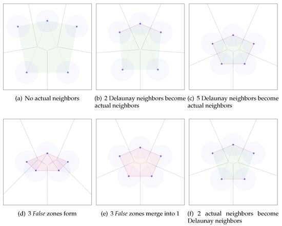
Figure 1. Evaluation of False and True zones with Adams algorithm. True zones marked green, False zones marked red. Delaunay neighbors shown with green edges, actual neighbors shown with red edges.

2.2. Distributing the Algorithm

As we argue in Section 2.3, it is enough for each node in a distributed setting to keep track of its Delaunay neighbors and their Delaunay neighbors. This observation motivates the following extension of Adams’ algorithm.

Each mobile sensor v needs to maintain a local extract $\mathcal{D}$ of the Delaunay graph of the nodes, with $DN\left(v\right)$ representing Delaunay neighbors, and $\alpha$-complex $\mathcal{A}$, with $N\left(v\right)$ denoting the $\alpha -complex$ neighbors. At each time tick $t_i$, each sensor v will update its location, perform the actions defined in Algorithm  2, and exchange messages with its neighbors $DN\left(v\right)$. We list all the possible events in Table 1.

Algorithm 2 Distributed Evasion Detection.

1: Send location update to $DN\left(v\right)$(broadcasting to $N\left(v\right)$, and via routing to $DN\left(v\right)-N\left(v\right)$). 2: Send neighbor’s current location to $DN\left(v\right)$. 3: Update Delaunay graph with most recent information from neighbors. 4: if Del-$\alpha$ then 5:     Notify all nodes on the boundary of the region that changes. 6: if$\alpha$-Del then 7:     Notify all nodes on the boundary of the region that changes. 8: if$\Delta$+ then 9:     Mark the triangle as True or False accordingly. 10: if Nbr+ then 11:     Sensor v becomes neighbor with u, u and v exchange the list of neighbors, and notify their neighbors the location of new neighbor. 12: if Nbr- then 13:     Sensor v loses its neighbor u(and vice versa), u and v notify their neighbors the updated list of neighbors.

Table 1. Events triggered by location update.

Symbols	Events
Del-$\alpha$	a Delaunay-edge becomes an $\alpha$-edge.
$\alpha$-Del	an $\alpha$-edge becomes a Delaunay-edge.
$\Delta$+	a triangle is added (Voronoi vertex is within $ϵ$ of all vertices).
$\Delta$-	a triangle disappears.
Nbr+	a new Delaunay neighbor appears.
Nbr-	a Delaunay neighbor disappears.

To compute $\mathcal{D}$ and $\mathcal{A}$, two-hop neighbor information will be used, and thus each sensor only need to communicate with its Delaunay neighbors, we will show that 2-hop neighbor information is suffice for our purpose in Section 2.3.

2.2.1. Tracked Information

Each node in the distributed system needs to independently keep track of:

• Its own location
• Locations of its neighbors and the neighbors’ neighbors
• A Voronoi diagram of these locations
• A Delaunay complex of these locations
• An $\alpha$-complex generated by the Delaunay complex and the sensing range $\alpha$
• For each region in the (planar) $\alpha$-complex graph,

  -

  Whether that region is labelled False or True

  -

  What the nodes along the boundary of that region are

• A list of neighbors $DN\left(v\right)$ in the Delaunay graph
• A list of neighbors $N\left(v\right)$ in the $\alpha$-complex
• A list of two-hop neighbors in the $\alpha$-complex

These pieces of information are updated as the event-driven algorithm continues—and if at the end of a time-span, any node tracks any region labelled True, then an evasion path exists. If all nodes only track regions labelled False, then no evasion path is possible.

2.2.2. Initial Phase

To bootstrap the process, each sensor v first will broadcast its location to all of its $\alpha -complex$ neighbors $N\left(v\right)$ with no neighbor information, so that every sensor will be able to establish a list of neighbors $N\left(v\right)$. At next time tick, sensors will exchange their neighbor list, and then calculate $N\left(v\right)$, $DN\left(v\right)$ and regions that exist in the network. A region is marked as True or False, depending on whether all sensors surrounding the region entirely cover the region. Coverage can be determined for a triangle in the $\alpha$-complex by checking whether the corresponding Voronoi vertex is within the covering range of all of the adjacent nodes.

2.2.3. Location Update

Each sensor v needs to update its Delaunay neighbors with its location and recompute its local Voronoi diagram and local Delaunay complex. Using the changes in the Delaunay complex observed from this update, the events listed in Table 1 trigger. This message also serves as heartbeat messages for detection of sensor failure. Location update messages will be exchanged with Delaunay neighbors every $\delta$ seconds, and upon receiving the location update, each sensor will update its neighbor information, and evaluate if any of the events-driven messages need to be sent out, as we are going to discuss in Section 2.2.4.

2.2.4. Event-Driven Messages

As defined in Table 1, the possible events that are caused by the change of underlying network topology need to be processed by each sensor and corresponding notifications should be sent to the neighbors.

2.2.5. Neighbor Changes

When the local Delaunay graph $\mathcal{D}$ and the local $\alpha$-complex $\mathcal{A}$ update, there are two ways that the neighborhood of a node itself can change: either a vertex leaves the two-hop neighborhood, or a vertex enters the two-hop neighborhood. If a neighbor leaves the one-hop neighborhood of a vertex v, this could mean it leaves the two-hop neighborhood of an adjacent vertex u resulting in the Nbr-event. v notifies all its neighbors of the change in its one-hop neighborhood. If a neighbor enters the one-hop neighborhood of a vertex v (from having been a two-hop neighbor), this could mean it enters the two-hop neighborhood of an adjacent vertex u resulting in the Nbr+ event. v notifies all its neighbors of the change in its one-hop neighborhood. In both cases, an updated one-hop neighborhood $DN\left(V\right)$ is communicated to all neighbors together with the updated locations of all the neighboring sensors.

2.2.6. Edge Changes

When sensors move around, if one sensor u moves out of the covered range of its neighbor v, but still remains a Delaunay neighbor, this triggers event $\alpha$-Del(u, v), which results in two regions merging into one, such that all sensors on both regions need to be notified for this merge. On the other hand, when one sensor u moves into the covered range of its Delaunay neighbor v, this triggers Del-$\alpha$(u, v), which results in one region splitting into two smaller regions, and all the sensors covering the region need to be notified for this split.

2.2.7. Region Changes

If a triangle emerges in the Delaunay graph, the status of this region is determined by whether the coverage area of all three sensors have non-empty intersections. If all three sensors intersect at some point in the middle, then we can mark the region of those three vertices as False and thus removed from the list of regions. It is enough to check the Voronoi vertex corresponding to the Delaunay simplex. It is also possible for a triangle disappears in the graph, but that would be constitute an edge change and is already covered by that event.

2.2.8. Routing Protocol

In a distributed algorithm, messages are required to be exchanged among Delaunay neighbors which are possibly laying out of communication ranges of the sensors. In this case, the message needs to be routed through the network. As discussed in  [18], the GPSR protocol [19] is able to route the message given location information of the sensors. It is also particularly useful to compute the Voronoi diagram distributively. Since location information of sensors is available in our system, we are adopting the same approach into our protocol. To apply the GPSR protocol, a planar communication graph is used. Since the sensor coverage graph $\mathcal{A}$ is planar, this graph can be used—otherwise the Relative Neighbor Graph [20] is a common choice. A message will first attempt to be delivered to the neighbor closest to the destination. If no such neighbor exists, there is a “void” region in the communication graph that needs to be circumnavigated. The GPSR protocol specifies to forward the message to the first neighbor in $\mathcal{A}$ in counterclockwise order, adopting a right-hand rule.

2.2.9. Examples

Figure 2 shows a running example of the distributed algorithm. In the local view figures, the red dot denotes the sensor we observed from, purple dots denote its Delaunay neighbors and blue dots denote the two-hop Delaunay neighbors. During the bootstrap phase, the sensor collects information from the entire network and computes a Voronoi diagram from its local view. After the bootstrap process, it will only communicate with its Delaunay neighbors and keep information on its two-hop Delaunay neighbors. As we can see from the figure that local Voronoi diagram does differ from the global view, due to the two-hop limit and the delay on the location update. However, the calculation of Delaunay neighbors is not affected, which is the key to our algorithm. Then it will calculate and update the Delaunay neighbors and regions accordingly.

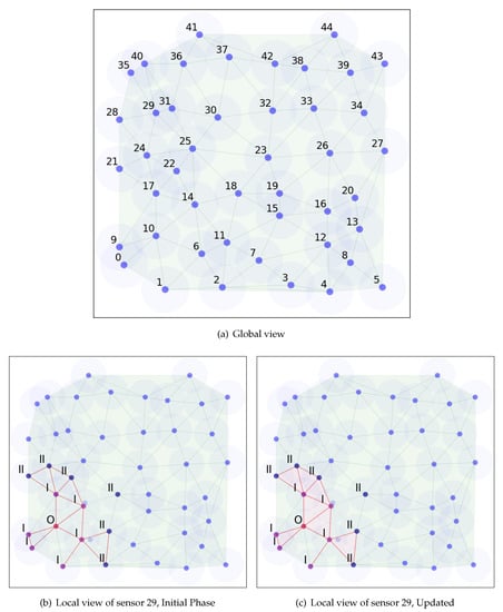
Figure 2. Running example of distributed algorithm.

Now let us consider the example in Figure 1, and label the nodes clockwise from the top as $a,b,c,d,e$. In step (c), all five nodes are tracking the same region $[a,b,c,d,e]$ as the (enclosed) region they are adjacent to. When moving from (c) to (d), two new edges grow shorter, causing $Del-\alpha$-updates introducing the edges $ac$ and $ad$. As $ac$ is introduced, node a takes responsibility to notify all five nodes of the change in regions: a, b and c are informed of the new region being $[a,b,c]$ while $a,c,d,e$ are informed of the new region being $[a,c,d,e]$ (a and c—as they are part of the same new edge—receive two new regions to track). When $ad$ is introduced, a informs $a,c,d$ of the new region $[a,c,d]$ and $a,d,e$ of the new region $[a,d,e]$.

By the time that step (d) is reached, all three of the resulting triangular regions have also come close enough to their respective Voronoi vertices to trigger the event $\Delta +$, labeling the three regions—independently of each other—with the label False which denotes the impossibility of an evasion path within them.

As we go from (d) to (e) in Figure 1, the two edges $ac$ and $ad$ grow too long for the $\alpha$-complex, and trigger one $\alpha -Del$ event each. As $ac$ triggers its event, the node a takes responsibility to inform $a,b,c,d$ that the regions $[a,b,c]$ and $[a,c,d]$ have merged into a region $[a,b,c,d]$ and that since both regions were labelled False, so is the new region. Then when $ad$ triggers its event, the node a again informs all the nodes that the regions $[a,b,c,d]$ and $[a,d,e]$ have merged into a single region $[a,b,c,d,e]$ which again inherits the labeling False from both regions having been labelled False.

2.3. Two Hop Neighbors Suffice

It is known from the theory of Delaunay triangulations [21] that if every edge of a graph is locally Delaunay, then the entire graph is the 1-skeleton of a Delaunay graph. Here, an edge $ab$ is locally Delaunay if it either is a boundary edge of the convex hull of the nodes, or it belongs to two triangles $abc$, $abd$ and d is outside the circumcircle of $abc$.

For a node a, checking whether an edge $ab$ is locally Delaunay will not involve any information further away than two hops through the Delaunay graph: $ad$ might not exist, but $bd$ certainly will.

Comparing the Delaunay triangulation of the set of two-hop neighbors of a to the Delaunay triangulation of all nodes, edges that connect two-hop neighbors might be erroneous due to nodes further away from a, but all edges that have at least one one-hop neighbor as a node agree between the local and global Delaunay triangulations.

2.4. Enumerating Evasion Paths

Once the full history is known, the data structures and changes in representation along the way allow us to enumerate all possible evasion paths.

2.4.1. Backwards Propagation

Each region labelled True in the final state corresponds to one group of path equivalence classes. As we replay the history of the algorithm from the end and backwards toward the beginning, every Merge event, where two regions $A_1,A_2$ labelled True become a single region R by the removal of an $\alpha$-complex edge splitting all the path equivalence classes that pass through R into two path equivalence classes each—one that came to R from $A_1$, and one that came from $A_2$. We describe this in Algorithm 3.

Algorithm 3 Evasion paths enumeration through backward propagation.

Given: A full history of an Evasion Detection using either Algorithm 1 or Algorithm 2. 1: Build a set ${\left\{G_i\right\}}_{i=1..N}$ of paths of height zero, one for each Alive region at time T   ▹ Initialization 2: for timestep $t=T..1$ in reverse do 3:     for path $G=[A_j,A_{j+1},\cdots ,A_T]$ do 4:         if $A_j$ is the product of merging two alive regions A and B then 5:            Duplicate G, prepending A to one copy and B to the other 6:         if all other cases then 7:            Prepend the Alive region from time step $j-1$ containing $A_j$ to the path G 8: Return the set of paths

2.4.2. Forwards Propagation

We can also track possible evasion paths in an online fashion—moving forwards in time as we track paths. Doing this, however, we are forced to represent more paths than those that may survive to the end, and need to prune the graph of possible path equivalence classes as regions transition from True to False. Any path that leads to such a transitioning region will have to be removed from further consideration. We describe this in Algorithm 4.

Algorithm 4 Evasion paths enumeration through forward propagation.

1: Build a set ${\left\{G_i\right\}}_{i=1\dots N}$ of trees of height zero, s.t. $i^{\mathrm{th}}$True region is a root of $G_i$.       ▹ Initialization 2: for timestep $t\in T$ do                                   ▹ Iteration 3:     if A region in the leaf $v_j$ of $G_i$ becomes False then 4:         Iteratively prune parent nodes of $v_j$ until we hit $v_k$ with a least 2 children. 5:     if A region in the leaf $v_j$ of $G_i$ splits into two regions then 6:         Create two children nodes $v_{j+1}$ and $v_{j+2}$ each containing 1 new region. 7:     if all other cases then 8:         Create child nodes of each leaf node tracking the regions of the child nodes.

2.4.3. Examples

We will use two simple examples of the evasion path algorithm in action to illustrate the evasion path enumeration algorithm variations.

The evasion path log that we will use for the forward propagation is depicted in Figure 3: a single enclosed region X gets split into two regions A and B, each of which is split again into A and $A^{\prime }$, B and $B^{\prime }$. Finally, two of the resulting four regions are covered by sensors, killing the corresponding region.

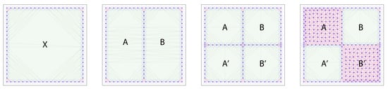
Figure 3. Forward propagation example progression of the evasion path algorithm. A single enclosed region gets split into two, each of which gets subsequently split into two regions each. Next, two of the four resulting regions die. A forward propagation evasion path enumeration will keep track of all homotopy classes of paths, and then prune the graph of possible evasion paths.

For the forward propagation, the algorithm goes through the following steps:

Time step	Evasion path list
1	$\left[X\right]$
2	$[X,A]$, $[X,B]$
3	$[X,A,A]$, $[X,A,A^{\prime }]$, $[X,B,B]$, $[X,B,B^{\prime }]$
4	$[X,A,A^{\prime },A^{\prime }]$, $[X,B,B,B]$

The graph grows, tracking more and more possible paths through the graph, until the regions A and $B^{\prime }$ die, at which point it is pruned back, discarding the evasion path classes that no longer are possible because they lead into dead ends.

In the backward propagation case, we use the example depicted in Figure 4: a single enclosed region X gets split into two regions A and B, each of which is split again into A and $A^{\prime }$, B and $B^{\prime }$. Finally, the regions are pairwise merged again into Y from A and B and $Y^{\prime }$ from $A^{\prime }$ and $B^{\prime }$.

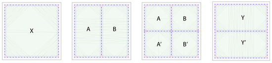
Figure 4. Backward propagation example progression of the evasion path algorithm. A single enclosed region gets split into two, each of which gets subsequently split into two regions each. Next, the resulting regions merge pairwise. A backward propagation evasion path enumeration will keep track of paths from the final True regions, copying the paths whenever a merge event is encountered, and tracking the paths backward otherwise.

The information tracked through the algorithm looks as follows:

Time step	Evasion path list
4	$\left[Y\right]$, $\left[Y^{\prime }\right]$
3	$[A,Y]$, $[B,Y]$, $[A^{\prime },Y^{\prime }]$, $[B^{\prime },Y^{\prime }]$
2	$[A,A,Y]$, $[B,B,Y]$, $[A,A^{\prime },Y^{\prime }]$, $[B,B^{\prime },Y^{\prime }]$
1	$[X,A,A,Y]$, $[X,B,B,Y]$, $[X,A,A^{\prime },Y^{\prime }]$, $[X,B,B^{\prime },Y^{\prime }]$

3. Discussion

In this work, we proposed an event-driven distributed algorithm that extends Adams’ evasion path detection algorithm [2]. Sensors with limited information from their neighbors can collaboratively track the existence or non-existence of an evasion path through a motion pattern. Evasion path algorithms are most closely related to classical coverage problems in sensor networks research but differ fundamentally in that the sensors are kept mobile, and the coverage criteria are adapted to this dynamic situation. With our adaptation, it is possible to implement the algorithm as a distributed sensor network system.

We also developed two algorithms to enumerate all possible evasion paths (up to homotopy)—one with a forward pass and one with a backward pass. The backward pass reviews the history of the motion pattern and is economical with its computation, since only paths that actually lead to the end are considered. The forward pass algorithm could be executed simultaneously with Adams’ or our algorithm to produce evasion path enumeration in an online fashion.

In the future work, we plan to accomplish both implementations and applications of our algorithm. As a first future step, we will implement the algorithm in a simulated environment and evaluate the performance with respect to multiple metrics—we have yet to determine what specific metrics to use. We also plan to apply the evasion path detection system for evaluating the search strategies. As additional information for a search strategy, the region tracking scheme in both Adams’ and our algorithms should mark redundancies and critical memberships in a search team. Using this information, a search strategy could reallocate resources to cover more ground in shorter time, with less movement and a lower probability of evasion without losing track of the regions already cleared by the search team. In addition, by measuring the area of the False regions, we will get a new metric for evaluating specific search strategies.

References

- De Silva, V.; Ghrist, R. Coordinate-Free Coverage in Sensor Networks with Controlled Boundaries via Homology. Int. J. Robot. Res. 2006, 25, 1205–1222. [Google Scholar] [CrossRef]
- Adams, H.; Carlsson, G. Evasion paths in mobile sensor networks. Int. J. Robot. Res. 2015, 34, 90–104. [Google Scholar] [CrossRef]
- Ghrist, R.; Krishnan, S. Positive Alexander Duality for Pursuit and Evasion. SIAM J. Appl. Algebra Geom. 2017, 1, 308–327. [Google Scholar] [CrossRef]
- Zhu, C.; Zheng, C.; Shu, L.; Han, G. A survey on coverage and connectivity issues in wireless sensor networks. J. Netw. Comput. Appl. 2012, 35, 619–632. [Google Scholar] [CrossRef]
- Mohamed, S.M.; Hamza, H.S.; Saroit, I.A. Coverage in Mobile Wireless Sensor Networks (M-WSN). Comput. Commun. 2017, 110, 133–150. [Google Scholar] [CrossRef]
- Zhang, H.; Hou, J.C. Maintaining sensing coverage and connectivity in large sensor networks. Ad Hoc Sens. Wirel. Netw. 2005, 1, 89–124. [Google Scholar]
- Huang, C.F.; Tseng, Y.C. The Coverage Problem in a Wireless Sensor Network. Mob. Netw. Appl. 2005, 10, 519–528. [Google Scholar] [CrossRef]
- Wang, X.; Xing, G.; Zhang, Y.; Lu, C.; Pless, R.; Gill, C. Integrated coverage and connectivity configuration in wireless sensor networks. In Proceedings of the 1st International Conference on Embedded Networked Sensor Systems, Los Angeles, CA, USA, 5–7 November 2003; pp. 28–39. [Google Scholar]
- Chaudhary, M.; Pujari, A.K. Q-Coverage Problem in Wireless Sensor Networks. In Distributed Computing and Networking; Garg, V., Wattenhofer, R., Kothapalli, K., Eds.; Springer: Berlin, Germany, 2009; pp. 325–330. [Google Scholar]
- Tao, D.; Wu, T.Y. A Survey on Barrier Coverage Problem in Directional Sensor Networks. IEEE Sens. J. 2015, 15, 876–885. [Google Scholar]
- Li, M.; Cheng, W.; Liu, K.; He, Y.; Li, X.; Liao, X. Sweep Coverage with Mobile Sensors. IEEE Trans. Mob. Comput. 2011, 10, 1534–1545. [Google Scholar]
- De Silva, V.; Ghrist, R. Coverage in Sensor Networks via Persistent Homology. Algebr. Geomet. Topol. 2007, 7, 339–358. [Google Scholar] [CrossRef]
- De Silva, V.; Ghrist, R. Homological Sensor Networks. Not. Am. Math. Soc. 2007, 54, 10–17. [Google Scholar]
- Dłotko, P.; Ghrist, R.; Juda, M.; Mrozek, M. Distributed computation of coverage in sensor networks by homological methods. Appl. Algebra Eng. Commun. Comput. 2012, 23, 29–58. [Google Scholar] [CrossRef]
- Gamble, J.; Chintakunta, H.; Krim, H. Applied Topology in Static and Dynamic Sensor Networks. In Proceedings of the International Conference on Signal Processing and Communications (SPCOM), Bangalore, India, 22–25 July 2012; pp. 1–5. [Google Scholar]
- Senouci, M.R.; Mellouk, A.; Asnoune, K.; Bouhidel, F.Y. Movement-Assisted Sensor Deployment Algorithms: A Survey and Taxonomy. IEEE Commun. Surv. Tutor. 2015, 17, 2493–2510. [Google Scholar] [CrossRef]
- Senouci, M.R.; Mellouk, A.; Assnoune, K. Localized Movement-Assisted SensorDeployment Algorithm for HoleDetection and Healing. IEEE Trans. Parallel. Distr. Syst. 2014, 25, 1267–1277. [Google Scholar] [CrossRef]
- Alsalih, W.; Islam, K.; Núñez Rodríguez, Y.; Xiao, H. Distributed Voronoi Diagram Computation in Wireless Sensor Networks. In Proceedings of the Twentieth Annual Symposium on Parallelism in Algorithms and Architectures, New York, NY, USA, 14–16 June 2008; p. 364. [Google Scholar]
- Karp, B.; Kung, H.T. GPSR: Greedy perimeter stateless routing for wireless networks. In Proceedings of the 6th annual international conference on Mobile computing and networking, Boston, MA, USA, 1 August 2000; pp. 243–254. [Google Scholar]
- Lingas, A. A linear-time construction of the relative neighborhood graph from the Delaunay triangulation. Comput. Geom. 1994, 4, 199–208. [Google Scholar] [CrossRef]
- Edelsbrunner, H. Geometry and Topology for Mesh Generation; Cambridge University Press: Cambridge, UK, 2001. [Google Scholar]
© 2020 by the authors. Licensee MDPI, Basel, Switzerland. This article is an open access article distributed under the terms and conditions of the Creative Commons Attribution (CC BY) license (http://creativecommons.org/licenses/by/4.0/).