Mining Sequential Patterns with VC-Dimension and Rademacher Complexity

Abstract

Sequential pattern mining is a fundamental data mining task with application in several domains. We study two variants of this task—the first is the extraction of frequent sequential patterns, whose frequency in a dataset of sequential transactions is higher than a user-provided threshold; the second is the mining of true frequent sequential patterns, which appear with probability above a user-defined threshold in transactions drawn from the generative process underlying the data. We present the first sampling-based algorithm to mine, with high confidence, a rigorous approximation of the frequent sequential patterns from massive datasets. We also present the first algorithms to mine approximations of the true frequent sequential patterns with rigorous guarantees on the quality of the output. Our algorithms are based on novel applications of Vapnik-Chervonenkis dimension and Rademacher complexity, advanced tools from statistical learning theory, to sequential pattern mining. Our extensive experimental evaluation shows that our algorithms provide high-quality approximations for both problems we consider.

1. Introduction

Sequential pattern mining [1] is a fundamental task in data mining and knowledge discovery, with applications in several fields, from recommender systems and e-commerce to biology and medicine. In its original formulation, sequential pattern mining requires to identify all frequent sequential patterns, that is, sequences of itemsets that appear in a fraction at least $\theta$ of all the transactions in a transactional dataset, where each transaction is a sequence of itemsets. The threshold $\theta$ is a user-specified parameter and its choice must be, at least in part, be informed by domain knowledge. In general, sequential patterns describe sequences of events or actions that are useful for predictions in many scenarios.

Several exact methods have been proposed to find frequent sequential patterns. However, the exact solution of the problem requires processing the entire dataset at least once, and often multiple times. For large, modern sized datasets, this may be infeasible. A natural solution to reduce the computation is to use sampling to obtain a small random portion (sample) of the dataset, and perform the mining process only on the sample. It is easy to see that by analyzing only a sample of the data the problem cannot be solved exactly, and one has to rely on the approximation provided by the results of the mining task on the sample. Therefore, the main challenge in using sampling is on computing a sample size such that the frequency of the sequential patterns in the sample is close to the frequency that would be obtained from the analysis on the whole dataset. Relating the two quantities using standard techniques (e.g., Hoeffding inequality and union bounds) does not provide useful results, that is, small sample sizes. In fact, such procedures require the knowledge of the number of all the sequential patterns in the dataset, which is impractical to compute in a reasonable time. So, one has to resort to loose upper bounds that usually result in sample sizes that are larger than the whole dataset. Recently, tools from statistical learning (e.g.,Vapnik-Chervonenkis dimension [2] and Rademacher complexity [3]) have been successfully used in frequent itemsets mining [4,5], a frequent pattern mining task where transactions are collections of items, showing that accurate and rigorous approximations can be obtained from small samples of the entire dataset. While sampling has previously been used in the context of sequential pattern mining (e.g., Reference [6]), to the best of our knowledge no sampling algorithm providing a rigorous approximation of the frequent sequential patterns has been proposed.

In several applications, the analysis of a dataset is performed to gain insight on the underlying generative process of the data. For example, in market basket analysis one is interested in gaining knowledge on the behaviour of all the customers, which can be modelled as a generative process from which the transactions in the dataset have been drawn. In such a scenario, one is not interested in sequential patterns that are frequent in the dataset, but in sequential patterns that are frequent in the generative process, that is, whose probability of appearing in a transaction generated from the process is above a threshold $\theta$. Such patterns, called true frequent patterns, have been introduced by Reference [7], which provides a Vapnik-Chervonenkis (VC) dimension based approach to mine true frequent itemsets. While there is a relation between the probability that a pattern appears in a transaction generated from the process and its frequency in the dataset, one cannot simply look at patterns with frequency above $\theta$ in the dataset to find the ones with probability above $\theta$ in the process. Moreover, due to the stochastic nature of the data, one cannot identify the true frequent patterns with certainty, and approximations are to be sought. In such a scenario, relating the probability that a pattern appears in a transaction generated from the process with its frequency in the dataset using standard techniques is even more challenging. Hoeffding inequality and union bounds require to bound the number of all the possible sequential patterns that can be generated from the process. Such bound is infinite if one considers all possible sequential patterns (e.g., does not bound the pattern length). To the best of our knowledge, no method to mine true frequent sequential patterns has been proposed.

1.1. Our Contributions

In this work, we study two problems in sequential pattern mining—mining frequent sequential patterns and mining true frequent sequential patterns. We propose efficient algorithms for these problems, based on the concepts of VC-dimension and Rademacher complexity. In this regard, our contributions are:

• We define rigorous approximations of the set of frequent sequential patterns and the set of true frequent sequential patterns. In particular, for both sets we define two approximations: one with no false negatives, that is, containing all elements of the set; and one with no false positives, that is, without any element that is not in the set. Our approximations are defined in terms of a single parameter, which controls the accuracy of the approximation and is easily interpretable.
• We study the VC-dimension and the Rademacher complexity of sequential patterns, two advanced concepts from statistical learning theory that have been used in other mining contexts, and provide algorithms to efficiently compute upper bounds for both. In particular, we provide a simple, but still effective in practice, upper bound to the VC-dimension of sequential patterns by relaxing the upper bound previously defined in Reference [8]. We also provide the first efficiently computable upper bound to the Rademacher complexity of sequential patterns. We also show how to approximate the Rademacher complexity of sequential patterns.
• We introduce a new sampling-based algorithm to identify rigorous approximations of the frequent sequential patterns with probability $1-\delta$, where $\delta$ is a confidence parameter set by the user. Our algorithm hinges on our novel bound on the VC-dimension of sequential patterns, and it allows to obtain a rigorous approximation of the frequent sequential patterns by mining only a fraction of the whole dataset.
• We introduce efficient algorithms to obtain rigorous approximations of the true frequent sequential patterns with probability $1-\delta$, where $\delta$ is a confidence parameter set by the user. Our algorithms use the novel bounds on the VC-dimension and on Rademacher complexity that we have derived, and they allow to obtain accurate approximations of the true frequent sequential patterns, where the accuracy depends on the size of the available data.
• We perform an extensive experimental evaluation analyzing several sequential datasets, showing that our algorithms provide high-quality approximations, even better than guaranteed by their theoretical analysis, for both tasks we consider.

1.2. Related Work

Since the introduction of the frequent sequential pattern mining problem [1], a number of exact algorithms has been proposed for this task, ranging from multi-pass algorithms using the anti-monotonicity property of the frequency function [9], to prefix-based approaches [10], to works focusing on the closed frequent sequences [11].

The use of sampling to reduce the amount of data for the mining process while obtaining rigorous approximations of the collection of interesting patterns has been successfully applied in many mining tasks. Raïssi and Poncelet [6] provided a theoretical bound on the sample size for a single sequential pattern in a static dataset using Hoeffding concentration inequalities, and they introduced a sampling approach to build a dynamic sample in a streaming scenario using a biased reservoir sampling. Our work is heavily inspired by the work of Riondato and Upfal [4,5], which introduced advanced statistical learning techniques for the task of frequent itemsets and association rules mining. In particular, in Reference [4] they employed the concept of VC-dimension to derive a bound on the sample size needed to obtain an approximation of the frequent itemsets and association rules from a dataset, while in Reference [5] they proposed a progressive sampling approach based on an efficiently computable upper bound on the Rademacher complexity of itemsets. VC-dimension has also been used to approximate frequent substrings in collections of strings [12], and the related concept of pseudo-dimension has been used to mine interesting subgroups [13]. Rademacher complexity has also been used in graph mining [14,15,16], to design random sampling approaches for estimating betweenness centralities in graphs [17].

Other works have studied the problem of approximating frequent sequential patterns using approaches other than sampling. In Reference [18], the dataset is processed in blocks with a streaming algorithm, but the intermediate sequential patterns returned may miss many frequent sequential patterns. More recently, Reference [8] introduced an algorithm to process the datasets in blocks using a variable, data-dependent frequency threshold, based on an upper bound to the empirical VC-dimension, to mine each block. Reference [8] defines an approximation for frequent sequential patterns that is one of the definitions we consider in this work. The intermediate results obtained after analyzing each block have probabilistic approximation guarantees, and after analyzing all blocks the output is the exact collection of frequent sequential patterns. While these works, in particular Reference [8], are related to our contributions, they do not provide sampling algorithms for sequential pattern mining.

To the best of our knowledge, Reference [7] is the only work that considers the extraction of frequent patterns w.r.t. an underlying generative process, based on the concept of empirical VC-dimension of itemsets. While we use the general framework introduced by Reference [7], the solution proposed by Reference [7] requires to solve an optimization problem that is tailored to itemsets and, thus, not applicable to sequential patterns; in addition, computing the solution of such problem could be relatively expensive. Reference [19] considers the problem of mining significant patterns under a similar framework, making more realistic assumptions on the underlying generative process compared to commonly used tests (e.g., Fisher’s exact test).

Several works have been proposed to identify statistically significant patterns where the significance is defined in terms of the comparison of patterns statistics. Few methods [20,21,22] have been proposed to mine statistically significant sequential patterns. These methods are orthogonal to our approach, which focuses on finding sequential patterns that are frequent with respect to (w.r.t.) an underlying generative distribution.

2. Preliminaries

We now provide the definitions and concepts used throughout the article. We start by introducing the task of sequential pattern mining and formally define the two problems which are the focus of this work: approximating the frequent sequential patterns and mining sequential patterns that are frequently generated from the underlying generative process. We then introduce two tools from statistical learning theory, that is, the VC-dimension and the Rademacher complexity, and the related concept of maximum deviation.

2.1. Sequential Pattern Mining

Let $\mathcal{I}=\{i_1,i_2,\cdots ,i_h\}$ be a finite set of elements called items. $\mathcal{I}$ is also called the ground set. An itemset P is a (non-empty) subset of $\mathcal{I}$, that is, $P\subseteq \mathcal{I}$. A sequential pattern $p=⟨P_1,P_2,\cdots ,P_{\mathcal{l}}⟩$ is a finite ordered sequence of itemsets, with $P_i\subseteq \mathcal{I},1\le i\le \mathcal{l}$. A sequential pattern p is also called a sequence. The length $\left|p\right|$ of p is defined as the number of itemsets in p. The item-length $\left|\right|p\left|\right|$ of p is the sum of the sizes of the itemsets in p, that is,

$$\left|\right|p\left|\right|=\sum _{i=1}^{\left|p\right|}\left|P_i\right|,$$

(1)

where $|P_i|$ is the number of items in itemset $P_i$. A sequence $a=⟨A_1,A_2,\cdots ,A_m⟩$ is a subsequence of another sequence $b=⟨B_1,B_2,$$\cdots ,B_n⟩$, denoted by $a⊑b$, if and only if there exist integers $1\le i_1<i_2<\cdots <i_m\le n$ such that $A_1\subseteq B_{i_1}$, $A_2\subseteq B_{i_2},\cdots ,A_m\subseteq B_{i_m}$. If a is a subsequence of b, then b is called a super-sequence of a, denoted by $b⊒a$.

Let $\mathbb{U}$ denote the set of all the sequences which can be built with itemsets containing items from $\mathcal{I}$. A dataset $\mathcal{D}$ is a finite bag of (sequential) transactions where each transaction is a sequence from $\mathbb{U}$. A sequence p belongs to a transaction $\tau \in \mathcal{D}$ if and only if $p⊑\tau$. For any sequence p, the support set $T_{\mathcal{D}}\left(p\right)$ of p in $\mathcal{D}$ is the set of transactions in $\mathcal{D}$ to which p belongs: $T_{\mathcal{D}}\left(p\right)=\{\tau \in D:p⊑\tau \}$. The support $Sup{p}_{\mathcal{D}}\left(p\right)$ of p in $\mathcal{D}$ is the cardinality of the set $T_{\mathcal{D}}\left(p\right)$, that is the number of transactions in $\mathcal{D}$ to which p belongs: $Sup{p}_{\mathcal{D}}\left(p\right)=\left|T_{\mathcal{D}}\left(p\right)\right|$. Finally, the frequency $f_{\mathcal{D}}\left(p\right)$ of p in $\mathcal{D}$ is the fraction of transactions in $\mathcal{D}$ to which p belongs:

$$f_{\mathcal{D}}\left(p\right)=\frac{Sup{p}_{\mathcal{D}}\left(p\right)}{\left|\mathcal{D}\right|}.$$

(2)

A sequence p is closed w.r.t. $\mathcal{D}$ if for each of its super-sequences $y⊐p$ we have $f_{\mathcal{D}}\left(y\right)<f_{\mathcal{D}}\left(p\right)$, or, equivalently, none of its super-sequence has support equal to $f_{\mathcal{D}}\left(p\right)$. We denote the set of all closed sequences in $\mathcal{D}$ with $CS\left(\mathcal{D}\right)$.

Example 1.

Consider the following dataset $\mathcal{D}=\{{\tau }_1,{\tau }_2,{\tau }_3,{\tau }_4\}$ as example:

$$\begin{array}{cc}\hfill & {\tau }_1=⟨\{6,7\},\left\{5\right\},\left\{7\right\},\left\{5\right\}⟩\hfill \\ \hfill & {\tau }_2=⟨\left\{1\right\},\left\{2\right\},\{6,7\},\left\{5\right\}⟩\hfill \\ \hfill & {\tau }_3=⟨\{1,4\},\left\{3\right\},\left\{2\right\},\{1,2,5,6\}⟩\hfill \\ \hfill & {\tau }_4=⟨\left\{1\right\},\left\{2\right\},\{6,7\},\left\{5\right\}⟩\hfill \end{array}$$

The dataset above has 4 transactions. The first one, ${\tau }_1=⟨\{6,7\},\left\{5\right\},\left\{7\right\},\left\{5\right\}⟩$, it is a sequence of length $|{\tau }_1|=4$ and item-length $\left|\right|{\tau }_1\left|\right|=5$. The frequency $f_{\mathcal{D}}\left(⟨\left\{7\right\},\left\{5\right\}⟩\right)$ of $⟨\left\{7\right\},\left\{5\right\}⟩$ in $\mathcal{D}$, is 3/4, since it is contained in all transactions but ${\tau }_3$. Note that the sequence $⟨\left\{7\right\},\left\{5\right\}⟩$ occurs three times as a subsequence of ${\tau }_1$, but ${\tau }_1$ contributes only once to the frequency of $⟨\left\{7\right\},\left\{5\right\}⟩$. The sequence $⟨\left\{7\right\},\left\{6\right\},\left\{5\right\}⟩$ is not a subsequence of ${\tau }_1$ because the order of the itemsets in the two sequences is not the same. Note that from the definitions above, an item can only occur once in an itemset, but it can occur multiple times in different itemsets of the same sequence. Finally, the sequence $⟨\{6,7\},\left\{5\right\}⟩$, whose frequency is 3/4, is a closed sequence, since its frequency is higher than the frequency of each of its super-sequences.

Section 2.1.1 and Section 2.1.2 formally define the two problems we are interested in.

2.1.1. Frequent Sequential Pattern Mining

Given a dataset $\mathcal{D}$ and a minimum frequency threshold $\theta \in (0,1]$, frequent sequential pattern (FSP) mining is the task of reporting the set $FSP(\mathcal{D},\theta )$ of all the sequences whose frequency in $\mathcal{D}$ is at least $\theta$, and their frequencies:

$$FSP(\mathcal{D},\theta )=\{(p,f_{\mathcal{D}}\left(p\right)):p\in \mathbb{U},f_{\mathcal{D}}\left(p\right)\ge \theta \}.$$

(3)

In the first part of this work, we are interested in finding the set $FSP(\mathcal{D},\theta )$ by only mining a sample of the dataset $\mathcal{D}$. Note that given a sample of the dataset $\mathcal{D}$, one cannot guarantee to find the exact set $FSP(\mathcal{D},\theta )$ and has to resort to approximations of $FSP(\mathcal{D},\theta )$. Thus, we are interested in finding rigorous approximations of $FSP(\mathcal{D},\theta )$. In particular, we consider the approximation of $FSP(\mathcal{D},\theta )$ defined in Reference [8].

Definition 1.

Given $\epsilon \in (0,1)$, an ε-approximation $\mathcal{C}$ of $FSP(\mathcal{D},\theta )$ is defined as a set of pairs $(p,f_p)$:

$$\mathcal{C}=\{(p,f_p):p\in \mathbb{U},f_p\in [0,1]\}$$

(4)

that has the following properties:

• $\mathcal{C}$ contains a pair $(p,f_p)$ for every $(p,f_{\mathcal{D}}\left(p\right))\in FSP(\mathcal{D},\theta )$;
• $\mathcal{C}$ contains no pair $(p,f_p)$ such that $f_{\mathcal{D}}\left(p\right)<\theta -\epsilon$;
• for every $(p,f_p)\in \mathcal{C}$, it holds $|f_{\mathcal{D}}\left(p\right)-f_p|\le \epsilon /2$.

(Note that while Reference [8] introduced the definition of $\epsilon$-approximation of $FSP(\mathcal{D},\theta )$, it did not provide a sampling algorithm to find such approximation for a given $\epsilon \in (0,1)$.)

Intuitively, the approximation $\mathcal{C}$ contains all the frequent sequential patterns that are in $FSP(\mathcal{D},\theta )$ (i.e., there are no false negatives) and no sequential pattern that has frequency in $\mathcal{D}$ much below $\theta$. In addition, $\mathcal{C}$ provides a good approximation of the actual frequency of the sequential pattern in $\mathcal{D}$, within an error $\epsilon /2$, arbitrarily small.

Depending on the application, one may be interested in a different approximation of $FSP(\mathcal{D},\theta )$, where all the sequential patterns in the approximation are frequent sequential patterns in the whole dataset.

Definition 2.

Given $\epsilon \in (0,1)$, a false positives free (FPF) ε-approximation $\mathcal{F}$ of $FSP(\mathcal{D},\theta )$ is defined as a set of pairs $(p,f_p)$:

$$\mathcal{F}=\{(p,f_p):p\in \mathbb{U},f_p\in [0,1]\}$$

(5)

that has the following properties:

• $\mathcal{F}$ contains no pair $(p,f_p)$ such that $f_{\mathcal{D}}\left(p\right)<\theta$;
• $\mathcal{F}$ contains all the pairs $(p,f_p)$ such that $f_{\mathcal{D}}\left(p\right)\ge \theta +\epsilon$;
• for every $(p,f_p)\in \mathcal{F}$, it holds $|f_{\mathcal{D}}\left(p\right)-f_p|\le \epsilon /2$.

The approximation $\mathcal{F}$ does not contain false positives, that is, sequences with $f_{\mathcal{D}}\left(p\right)<\theta$. In addition, it does not miss sequences with $f_{\mathcal{D}}\left(p\right)\ge \theta +\epsilon$ and, similarly to the $\epsilon$-approximation, we have that, for every pair in $\mathcal{F}$, it gives a good approximation of the actual frequency of the sequential patterns in $\mathcal{D}$, within an error $\epsilon /2$, arbitrarily small.

2.1.2. True Frequent Sequential Pattern Mining

In several applications, the dataset $\mathcal{D}$ is a sample of transactions independently drawn from an unknown probability distribution $\pi$ on $\mathbb{U}$. In such a scenario, the dataset $\mathcal{D}$ is a finite bag of $\left|\mathcal{D}\right|$ independent identically distributed (i.i.d.) samples from $\pi$. For any sequence $p\in \mathbb{U}$, the real support set $T\left(p\right)$ of p is the set of sequences in $\mathbb{U}$ to which p belongs: $T\left(p\right)=\{\tau \in \mathbb{U}:p⊑\tau \}$. We define the true frequency $t_{\pi }\left(p\right)$ of p w.r.t. $\pi$ as the probability that a transaction sampled from $\pi$ contains p:

$$t_{\pi }\left(p\right)=\sum _{\tau \in T\left(p\right)}\pi \left(\tau \right).$$

(6)

In this scenario, the final goal of the data mining process on $\mathcal{D}$ is to gain a better understanding of the process generating the data, that is, of the distribution $\pi$, through the true frequencies $t_{\pi }$, which are unknown and only approximately reflected in the dataset $\mathcal{D}$. Therefore, we are interested in finding the sequential patterns with true frequency $t_{\pi }$ at least $\theta$ for some $\theta \in (0,1]$. We call these sequential patterns the true frequent sequential patterns (TFSPs) and denote their set as:

$$TFSP(\pi ,\theta )=\{(p,t_{\pi }\left(p\right)):p\in \mathbb{U},t_{\pi }\left(p\right)\ge \theta \}.$$

(7)

Note that, given a finite number of random samples from $\pi$ (e.g., the dataset $\mathcal{D}$), it is not possible to find the exact set $TFSP(\pi ,\theta )$, and one has to resort to approximations of $TFSP(\pi ,\theta )$. Analogously to the two approximations defined for the FSPs, now we define two approximations of the TFSPs, depending on the application we are interested in: the first one that does not have false negatives, while the second one that does not contain false positives.

Definition 3.

Given $\mu \in (0,1)$, a μ-approximation $\mathcal{E}$ of $TFSP(\pi ,\theta )$ is defined as a set of pairs $(p,f_p)$:

$$\mathcal{E}=\{(p,f_p):p\in \mathbb{U},f_p\in [0,1]\}$$

(8)

that has the following properties:

• $\mathcal{E}$ contains a pair $(p,f_p)$ for every $(p,t_{\pi }\left(p\right))\in TFSP(\pi ,\theta )$;
• $\mathcal{E}$ contains no pair $(p,f_p)$ such that $t_{\pi }\left(p\right)<\theta -\mu$;
• for every $(p,f_p)\in \mathcal{E}$, it holds $|t_{\pi }\left(p\right)-f_p|\le \mu /2$.

Definition 4.

Given $\mu \in (0,1)$, a false positives free (FPF) μ-approximation $\mathcal{G}$ of $TFSP(\pi ,\theta )$ is defined as a set of pairs $(p,f_p)$:

$$\mathcal{G}=\{(p,f_p):p\in \mathbb{U},f_p\in [0,1]\}$$

(9)

that has the following properties:

• $\mathcal{G}$ contains no pair $(p,f_p)$ such that $t_{\pi }\left(p\right)<\theta$;
• $\mathcal{G}$ contains all the pairs $(p,f_p)$ such that $t_{\pi }\left(p\right)\ge \theta +\mu$;
• for every $(p,f_p)\in \mathcal{G}$, it holds $|t_{\pi }\left(p\right)-f_p|\le \mu /2$.

2.2. VC-Dimension

The Vapnik-Chervonenkis (VC) dimension [2,23] of a space of points is a measure of the complexity or expressiveness of a family of indicator functions, or, equivalently, of a family of subsets, defined on that space. A finite bound on the VC-dimension of a structure implies a bound of the number of random samples required to approximately learn that structure.

We define a range space as a pair $(X,\mathcal{R})$, where X is a finite or infinite set and $\mathcal{R}$, the range set, is a finite or infinite family of subsets of X. The members of X are called points, while the members of $\mathcal{R}$ are called ranges. Given $A\subseteq X$, we define the projection of $\mathcal{R}$ in A as $P_{\mathcal{R}}\left(A\right)=\{r\cap A:r\in \mathcal{R}\}$. We define $2^A$ as the power set of A, that is the set of all the possible subsets of A, including the empty set ∅ and A itself. If $P_{\mathcal{R}}\left(A\right)=2^A$, then A is said to be shattered by $\mathcal{R}$. The VC-dimension of a range space is the cardinality of the largest set shattered by the space.

Definition 5.

Let $RS=(X,\mathcal{R})$ be a range space and $B\subseteq X$. The empirical VC-dimension $EVC(RS,B)$ of $RS$ on B is the maximum cardinality of a subset of B shattered by $\mathcal{R}$. The VC-dimension $VC\left(RS\right)$ of $RS$ is defined as $VC\left(RS\right)=EVC(RS,X)$.

Example 2.

Let $X=[0,1]$ be the set of all the points in $[0,1]$ and let $\mathcal{R}$ be the set of subsets $[a,b]$, with $0\le a\le b\le 1$, that is $[a,b]\subseteq [0,1]$. Let us consider the set $Y=\{x,y,z\}$, containing 3 points $0\le x<y<z\le 1$. It is not possible to find a range whose intersection with the set Y is $\{x,z\}$, since all the ranges $[a,b]$, with $0\le a\le b\le 1$, containing x and z, also contain y. Then, $VC(X,\mathcal{R})$ must be less than 3. Consider now the set $Y=\{x,y\}$, containing only 2 points $0\le x<y\le 1$. It is easy to see that Y is shattered by $\mathcal{R}$, so $VC(X,\mathcal{R})=2$.

The main application of VC-dimension in statistics and learning theory is to derive the sample size needed to approximately “learn” the ranges, as defined below.

Definition 6.

Let $RS=(X,\mathcal{R})$ be a range space. Given $\epsilon \in (0,1)$, a bag B of elements taken from X is an ε-bag of X if for all $r\in \mathcal{R}$, we have

$$\left|\frac{|X\cap r|}{\left|X\right|}-\frac{|B\cap r|}{\left|B\right|}\right|\le \epsilon .$$

(10)

Theorem 1.

There is a constant $c>0$ such that if $(X,\mathcal{R})$ is a range space of VC-dimension $\le d$, and $\epsilon ,\delta \in (0,1)$, then a bag B of m elements taken with independent random extractions with replacement from X, where

$$m\ge \frac{c}{{\epsilon }^2}\left(d+ln\frac{1}{\delta }\right),$$

(11)

is an ε-bag of X with probability $\ge 1-\delta .$

The universal constant c has been experimentally estimated to be at most $0.5$ [24]. In the remaining of this work, we will use $c=0.5$. Note that Theorem 1 holds also when d is an upper bound to the empirical VC-dimension $EVC(RS,B)$ of $RS$ on B [25]. In that case, the bag B itself is an $\epsilon$-bag of X.

2.3. Rademacher Complexity

The Rademacher complexity [3,23,26] is a tool to measure the complexity of a family of real-valued functions. Bounds based on the Rademacher complexity depend on the distribution of the dataset, differently from the ones based on VC-dimension that are distribution independent.

Let $\mathcal{D}$ be a dataset of n transactions $\mathcal{D}=\{t_1,\cdots ,t_n\}$. For each $i\in \{1,\cdots ,n\}$, let ${\sigma }_i$ be an independent Rademacher random variable (r.v.) that takes value 1 or $-1$, each with probability $1/2$. Let $\mathcal{G}$ be a set of real-valued functions. The empirical Rademacher complexity $R_{\mathcal{D}}$ on $\mathcal{D}$ is defined as follows:

$$R_{\mathcal{D}}={\mathbb{E}}_{\sigma }\left[\underset{g\in \mathcal{G}}{sup}{\displaystyle \frac{1}{n}}\sum _{i=1}^n{\sigma }_{i}g\left(t_i\right)\right],$$

(12)

where the expectation is taken w.r.t. the Rademacher r.v. ${\sigma }_i$’s.

The Rademacher complexity is a measure of the expressiveness of the set $\mathcal{G}$. A specific combination of $\sigma$’s represents a splitting of $\mathcal{D}$ into two random sub-samples ${\mathcal{D}}_1$ and ${\mathcal{D}}_{-1}$. For a function $g\in \mathcal{G}$, ${\sum }_{i=1}^{n}g\left(t_i\right)/n$ represents a good approximation of $\mathbb{E}\left[g\right]$ over $\mathcal{D}$ if n is sufficiently large. ${\sum }_{i=1}^n{\sigma }_{i}g\left(t_i\right)/n$ represents instead the difference between $\mathbb{E}\left[g\right]$ over the two random sub-samples ${\mathcal{D}}_1$ and ${\mathcal{D}}_{-1}$. By considering the expected value of the supremum of this difference over the set $\mathcal{G}$, we get the empirical Rademacher complexity. Therefore, the intuition is that if $R_{\mathcal{D}}$ is small, the dataset $\mathcal{D}$ is sufficiently large to ensure a good estimate of $\mathbb{E}\left[g\right]$ for every $g\in \mathcal{G}$. In this work, we study the Rademacher complexity of sequential patterns, which has not been explored before.

2.4. Maximum Deviation

Let $\mathcal{M}$ be a probability distribution over a domain set $\mathcal{Z}$. Let $\mathcal{F}$ be a set of functions that go from $\mathcal{Z}$ to $[-1,1]$. Given a function $f\in \mathcal{F}$, we define the expectation of f as:

$$\mathbb{E}\left(f\right)={\mathbb{E}}_{z\sim \mathcal{M}}\left[f\left(z\right)\right],$$

(13)

and, given a sample Z of n observations $z_1,\cdots ,z_n$ drawn from $\mathcal{M}$, the empirical average of f on Z as:

$$E(f,Z)={\displaystyle \frac{1}{n}}\sum _{i=1}^{n}f\left(z_i\right).$$

(14)

The maximum deviation is defined as the largest difference between the expectation of a function f and its empirical average on sample Z as:

$$\underset{f\in \mathcal{F}}{sup}|\mathbb{E}\left(f\right)-E(f,Z)|.$$

(15)

We now use the maximum deviation to capture quantities of interest for the two mining tasks we consider in this work.

In the frequent pattern mining scenario, we aim to find good estimates for $f_{\mathcal{D}}\left(p\right)$ for each pattern p. The frequency $f_{\mathcal{D}}\left(p\right)$ is the expectation of a Bernoulli random variable (r.v.) $X_{\mathcal{D}}(p,t)$ which is 1 if the pattern p appears in a transaction t drawn uniformly at random from $\mathcal{D}$:

$${\mathbb{E}}_{t\sim \mathcal{D}}\left[X_{\mathcal{D}}(p,t)\right]=\underset{t\sim \mathcal{D}}{Pr}(X_{\mathcal{D}}(p,t)=1)=Sup{p}_{\mathcal{D}}\left(p\right)/\left|\mathcal{D}\right|=f_{\mathcal{D}}\left(p\right).$$

(16)

Let $\mathcal{S}$ be a sample of transactions drawn uniformly and independently at random from $\mathcal{D}$. We define the frequency $f_{\mathcal{S}}\left(p\right)$ as the fraction of transactions of $\mathcal{S}$ where p appears. In this scenario, we have that the frequency $f_{\mathcal{D}}\left(p\right)$ of p on $\mathcal{D}$ and the frequency $f_{\mathcal{S}}\left(p\right)$ of p on the sample $\mathcal{S}$ represent, respectively, the expectation $\mathbb{E}\left(f_p\right)$ and the empirical average $E(f_p,\mathcal{S})$ of a function $f_p$ associated with a pattern p. Thus, the maximum deviation is:

$$\underset{p\in \mathbb{U}}{sup}|f_{\mathcal{D}}\left(p\right)-f_{\mathcal{S}}\left(p\right)|.$$

(17)

In the true frequent pattern mining scenario, we aim to find good estimates for $t_{\pi }\left(p\right)$ for each pattern p. Note that the true frequency $t_{\pi }\left(p\right)$ is the expectation of a Bernoulli r.v. which is 1 if the pattern p appears in a transaction drawn from $\pi$. Moreover, it is easy to prove that the observed frequency $f_{\mathcal{D}}\left(p\right)$ of a pattern p in a dataset $\mathcal{D}$ of transactions drawn from $\pi$ is an unbiased estimator for $t_{\pi }\left(p\right)$, that is: $\mathbb{E}\left[f_{\mathcal{D}}\left(p\right)\right]=t_{\pi }\left(p\right)$.

Therefore, the true frequency $t_{\pi }\left(p\right)$ and the frequency $f_{\mathcal{D}}\left(p\right)$ observed on the dataset $\mathcal{D}$ represent, respectively, the expectation $\mathbb{E}\left(f_p\right)$ and the empirical average $E(f_p,\mathcal{D})$ of a function $f_p$ associated with a pattern p. Thus, the maximum deviation is:

$$\underset{p\in \mathbb{U}}{sup}|t_{\pi }\left(p\right)-f_{\mathcal{D}}\left(p\right)|.$$

(18)

In the next sections, we provide probabilistic upper bounds to the maximum deviation using the VC-dimension and Rademacher complexity which can therefore be used for frequent pattern mining and true frequent pattern mining scenarios.

3. VC-Dimension of Sequential Patterns

In this section, we apply the statistical learning theory concept of VC-dimension to sequential patterns. First, we define the range space associated with a sequential dataset. Then, we show a computable efficient upper bound on the VC-dimension and, finally, we present two applications of such upper bound. The first one is to compute the size of a sample that guarantees to obtain a good approximation for the problem of mining the frequent sequential patterns. The second one is to compute an upper bound on the maximum deviation to mine the true frequent sequential patterns.

Remember that a range space is a pair $(X,\mathcal{R})$ where X contains points and $\mathcal{R}$ contains ranges. For a sequential dataset, X is the dataset itself, while $\mathcal{R}$ contains the sequential transactions that are the support set for some sequential patterns.

Definition 7.

Let $\mathcal{D}$ be a sequential dataset consisting of sequential transactions and let $\mathcal{I}$ be its ground set. Let $\mathbb{U}$ be the set of all sequences built with itemsets containing item from $\mathcal{I}$. We define $RS=(X,\mathcal{R})$ to be a range space associated with $\mathcal{D}$ such that:

• $X=\mathcal{D}$ is the set of sequential transactions in the dataset;
• $\mathcal{R}=\{T_{\mathcal{D}}\left(p\right):p\in \mathbb{U}\}$ is a family of sets of sequential transactions such that for each sequential pattern p, the set $T_{\mathcal{D}}\left(p\right)=\{\tau \in \mathcal{D}:p⊑\tau \}$ is the support set of p on $\mathcal{D}$.

The VC-dimension of this range space is the maximum size of a set of sequential transactions that can be shattered by the support sets of the sequential patterns.

Example 3.

Consider the following dataset $\mathcal{D}=\{{\tau }_1,{\tau }_2,{\tau }_3,{\tau }_4\}$ as an example:

$$\begin{array}{cc}\hfill {\tau }_1& =⟨\left\{1\right\},\{2,3\},\{4,5,6\}⟩\hfill \\ \hfill {\tau }_2& =⟨\left\{1\right\},\left\{3\right\},\left\{4\right\}⟩\hfill \\ \hfill {\tau }_3& =⟨\left\{7\right\},\{3,4\}⟩\hfill \\ \hfill {\tau }_4& =⟨\left\{4\right\},\left\{5\right\}⟩\hfill \end{array}$$

The dataset above has 4 transactions. We now show that the VC-dimension of the range space $RS$ associated with $\mathcal{D}$ is 2. Let us consider the set $A=\{{\tau }_2,{\tau }_3\}$. The power set $2^A$ of A is $2^A=\{\varnothing ,\left\{{\tau }_2\right\},\left\{{\tau }_3\right\},\{{\tau }_2,{\tau }_3\}\}$. A is shatter by $\mathcal{R}$ since the projection $P_{\mathcal{R}}\left(A\right)$ of $\mathcal{R}$ in A is equal to $2^A$ (remember that $P_{\mathcal{R}}\left(A\right)=\{r\cap A:r\in \mathcal{R}\}$):

$$\begin{array}{cc}\hfill \varnothing & =A\cap T_{\mathcal{D}}\left(⟨\left\{6\right\}⟩\right),\hfill \\ \hfill \left\{{\tau }_2\right\}& =A\cap T_{\mathcal{D}}\left(⟨\left\{1\right\}⟩\right),\hfill \\ \hfill \left\{{\tau }_3\right\}& =A\cap T_{\mathcal{D}}\left(⟨\{3,4\}⟩\right),\hfill \\ \hfill A=\{{\tau }_2,{\tau }_3\}& =A\cap T_{\mathcal{D}}\left(⟨\left\{3\right\}⟩\right).\hfill \end{array}$$

Since $\left|A\right|=2$ and A is shattered by $\mathcal{R}$, then the range space associated with $\mathcal{D}$ has VC-dimension $\ge 2$. Analogously, the sets $\{{\tau }_1,{\tau }_3\}$,$\{{\tau }_1,{\tau }_4\}$,$\{{\tau }_2,{\tau }_4\}$ and $\{{\tau }_3,{\tau }_4\}$ are shattered by $\mathcal{R}$. The set $B=\{{\tau }_1,{\tau }_2\}$ is instead not shattered by $\mathcal{R}$: since ${\tau }_2⊑{\tau }_1$, there is not a sequential pattern $p^{*}$ such that $B\cap T_{\mathcal{D}}\left(p^{*}\right)=\left\{{\tau }_2\right\}$. The sets $C=\{{\tau }_1,{\tau }_3,{\tau }_4\}$ and $E=\{{\tau }_2,{\tau }_3,{\tau }_4\}$ are not shattered by $\mathcal{R}$ either: there is not a sequential pattern $p^{\prime }$ such that $\{{\tau }_3,{\tau }_4\}=C\cap T_{\mathcal{D}}\left(p^{\prime }\right)$ or $\{{\tau }_3,{\tau }_4\}=E\cap T_{\mathcal{D}}\left(p^{\prime }\right)$. Thus, the VC-dimension of the range space associated with $\mathcal{D}$ is exactly 2.

The exact computation of the (empirical) VC-dimension of the range space associated with a dataset $\mathcal{D}$ is computationally expensive. The s-index, introduced by Servan-Schreiber et al. [8], provides an efficiently computable upper bound on the VC-dimension of sequential patterns. Such upper bound is based on the notion of capacity $c\left(p\right)$ of a sequence p. The capacity $c\left(p\right)$ of a sequence p is the number of distinct subsequences of p, that is, $c\left(p\right)=\left|\right\{z:z⊑p\left\}\right|$. The exact capacity can be computed using the algorithm described in Reference [27], but it is computationally expensive and may be prohibitive for large datasets. Instead, Reference [8] proposed an algorithm to compute a more efficient upper bound $\tilde{c}\left(p\right)\ge c\left(p\right)$. Let us consider that a first simple bound is given by $2^{\left|\right|p\left|\right|}-1$, that may be a loose upper bound of $c\left(p\right)$ because it is obtained by considering all the items contained in all the itemsets in p as distinct, that is, the capacity of the sequence p is $2^{\left|\right|p\left|\right|}-1$ if and only if all the items contained in all the itemsets of the sequence p are different. The bound proposed by Reference [8] can be computed as follows. When p contains, among others, two itemsets A and B such that $A\subseteq B$, subsequences of the form $⟨C⟩$ with $C\subseteq A$ are considered twice in $2^{\left|\right|p\left|\right|}-1$, “generated” once from A and once from B. To avoid over-counting such $2^{\left|A\right|}-1$ subsequences, Reference [8] proposes to consider only the ones “generated” from the longest itemset that can generate them. Then, the s-index is defined as follows.

Definition 8

([8]). Let $\mathcal{D}$ be a sequential dataset. The s-index of $\mathcal{D}$ is the maximum integer s such that $\mathcal{D}$ contains at least s different sequential transactions with upper bound to their capacities $\tilde{c}\left(p\right)$ at least $2^s-1$, such that no one of them is a subset of another, that is the s sequential transactions form an anti-chain.

The following result from Reference [8] shows that the s-index is an upper bound to the VC-dimension of the range space for sequential patterns in $\mathcal{D}$.

Theorem 2

(Lemma 3 [8]). Let $\mathcal{D}$ be a sequential dataset with s-index s. Then, the range space $RS=(X,\mathcal{R})$ corresponding to $\mathcal{D}$ has VC-dimension $\le s$.

While an upper bound to the s-index can be computed in a streaming fashion, it still requires to check whether a transaction is a subset of the set of other transactions currently maintained in memory and that define the current value of the s-index. In addition, the computation of the upper bound $\tilde{c}\left(p\right)$ on the capacity of a sequence p requires to check whether the itemsets of p are subsets of each others. To avoid such expensive operations, we define an upper bound to the s-index, that we call s-bound, which does not require to check whether the transactions form an anti-chain.

Definition 9.

Let $\mathcal{D}$ be a sequential dataset. The s-bound of $\mathcal{D}$ is the maximum integer s such that $\mathcal{D}$ contains at least s different sequential transactions with item-length at least s.

Algorithm 1 shows the pseudo-code to compute an upper bound to the s-bound in a streaming fashion. It uses an ordered set to maintain in memory the set of transactions that define the current value of the s-bound. The ordered set stores pairs composed by a transaction and its item-length, sorted by decreasing item-length. In addition, it uses a hash set to speed up the control on the equal transactions.

In practice, it is quite uncommon that the long sequences that define the value of the s-index are subsequences of other sequences, thus, removing the anti-chain constraint, the bound does not deteriorate. In addition, the usage of the naive algorithm to compute the upper bound on $c\left(p\right)$, that is $2^{\left|\right|p\left|\right|}-1$, it is equivalent to consider the transactions that have item-length at least s to calculate the s-bound, making the computation much faster without worsening the bound on the VC-dimension in practice.

Algorithm1: SBoundUpp($\mathcal{D}$): computation of an upper bound on the s-bound.

3.1. Compute the Sample Size for Frequent Sequential Pattern Mining

In this section, we show how to compute a sample size m for a random sample S of transactions taken from $\mathcal{D}$ such that the maximum deviation is bounded by $\epsilon /2$, that is, ${sup}_{p\in \mathbb{U}}|f_{\mathcal{D}}\left(p\right)-f_S\left(p\right)|\le \epsilon /2$, for a user-defined value $\epsilon$, using the upper bound on the VC-dimension defined above. Such result underlies the sampling algorithm that will be introduced in Section 5. Algorithm 2 shows how to compute a sample size that guarantees that ${sup}_{p\in \mathbb{U}}|f_{\mathcal{D}}\left(p\right)-f_S\left(p\right)|\le \epsilon /2$ with probability $\ge 1-\delta$. This algorithm is used in the sampling algorithm (Section 5).

Theorem 3

(Proof in Appendix A). Let S be a random sample of m transactions taken with replacement from the sequential dataset $\mathcal{D}$ and $\epsilon ,\delta \in (0,1)$. Let d be the s-bound of $\mathcal{D}$. If

$$m\ge \frac{2}{{\epsilon }^2}\left(d+ln\frac{1}{\delta }\right),$$

(19)

then ${sup}_{p\in \mathbb{U}}|f_{\mathcal{D}}\left(p\right)-f_S\left(p\right)|\le \epsilon /2$ with probability at least $1-\delta$.

Algorithm2: ComputeSampleSize($\mathcal{D},\epsilon ,\delta$): computation of the sample size such that ${sup}_{p\in \mathbb{U}}|f_{\mathcal{D}}\left(p\right)-f_S\left(p\right)|\le \epsilon /2$ with probability $\ge 1-\delta$.

Data: Dataset $\mathcal{D}$; $\epsilon ,\delta \in (0,1)$.    Result: The sample size m. 1 $d\leftarrow$ SBoundUpp($\mathcal{D}$); 2 $m\leftarrow 2/{\epsilon }^2\left(d+ln(1/\delta )\right)$; 3 return m;

3.2. Compute an Upper Bound to the Max Deviation for the True Frequent Sequential Patterns

In this section, we show how to compute an upper bound on the maximum deviation ${\mu }_{VC}/2$ for the true frequent sequential pattern mining problem, that is, ${sup}_{p\in \mathbb{U}}|t_{\pi }\left(p\right)-f_{\mathcal{D}}\left(p\right)|\le {\mu }_{VC}/2$, using the upper bound on the empirical VC-dimension. Such result underlies the strategy for mining the true frequent sequential patterns that will be introduced in Section 6.

We define a range space associated with the generative process $\pi$ as a range space where the points $X=\mathbb{U}$ and the range set $\mathcal{R}=\left\{T\right(p):p\in \mathbb{U}\}$. The s-bound of the dataset $\mathcal{D}$, as defined above, is an upper bound on the empirical VC-dimension of the range space associated with $\pi$ computed on $\mathcal{D}$. Algorithm 3 shows how to compute an upper bound on the maximum deviation that is used in the true frequent sequential pattern mining algorithm (Section 6).

Theorem 4

(Proof in Appendix A). Let $\mathcal{D}$ be a finite bag of $\left|\mathcal{D}\right|$ i.i.d. samples from an unknown probability distribution π on $\mathbb{U}$ and $\delta \in (0,1)$. Let d be the s-bound of $\mathcal{D}$. If

$${\mu }_{VC}=\sqrt{\frac{2}{\left|\mathcal{D}\right|}\left(d+ln\frac{1}{\delta }\right)},$$

(20)

then ${sup}_{p\in \mathbb{U}}|t_{\pi }\left(p\right)-f_{\mathcal{D}}\left(p\right)|\le {\mu }_{VC}/2$ with probability at least $1-\delta$.

Algorithm3: ComputeMaxDevVC($\mathcal{D},\delta$): computation of an upper bound on the max deviation for the true frequent sequential pattern mining problem.

Data: Dataset $\mathcal{D}$; $\delta \in (0,1)$.    Result: Upper bound to the max deviation ${\mu }_{VC}/2$. 1 $d\leftarrow$ SBoundUpp($\mathcal{D}$); 2 ${\mu }_{VC}\leftarrow \sqrt{2/\left|\mathcal{D}\right|\left(d+ln(1/\delta )\right)}$; 3 return ${\mu }_{VC}/2$;

4. Rademacher Complexity of Sequential Patterns

In this section we introduce the Rademacher complexity of sequential patterns. We propose a method for finding an efficiently computable upper bound to the empirical Rademacher complexity $R_{\mathcal{D}}$ of sequential patterns (similar to what has been done in Reference [5] for itemsets) and a method for approximating it. In the true frequent pattern mining scenario, these results will be useful for defining a quantity which is an upper bound to the maximum deviation ${sup}_{p\in \mathbb{U}}|t_{\pi }\left(p\right)-f_{\mathcal{D}}\left(p\right)|$ with high probability.

The introduction of the Rademacher complexity of sequential patterns requires the definition of a set of real-valued functions. We define, for each pattern $p\in \mathbb{U}$, the indicator function ${\varphi }_p:\mathbb{U}\to \{0,1\}$ as:

$${\varphi }_p\left(t\right)=\left\{\begin{array}{cc}1\hfill & ifp⊑t\hfill \\ 0\hfill & otherwise\hfill \end{array}\right.,$$

(21)

where t is a transaction. Given a transaction t of a dataset $\mathcal{D}$ with n transactions, ${\varphi }_p\left(t\right)$ is 1 if p appears in t, otherwise it is 0. We define the set of real-valued functions as the family of these indicator functions. The frequency of p in $\mathcal{D}$ can be defined using the indicator function ${\varphi }_p$: $f_{\mathcal{D}}\left(p\right)={\sum }_{t\in \mathcal{D}}{\varphi }_p\left(t\right)/n.$ The (empirical) Rademacher complexity $R_{\mathcal{D}}$ on a given dataset $\mathcal{D}$ is defined as:

$$R_{\mathcal{D}}={\mathbb{E}}_{\sigma }\left[\underset{p\in \mathbb{U}}{sup}{\displaystyle \frac{1}{n}}\sum _{i=1}^n{\sigma }_i{\varphi }_p\left(t_i\right)\right],$$

(22)

where the expectation is taken w.r.t. the Rademacher r.v. ${\sigma }_i$, that is, conditionally on the dataset $\mathcal{D}$. The connection between the Rademacher complexity of sequential patterns and the maximum deviation is given by the following theorem, which derives from standard results in statistical learning theory (Thm. 3.2 in Reference [3]).

Theorem 5.

With probability at least $1-\delta$:

$$\underset{p\in \mathbb{U}}{sup}|t_{\pi }\left(p\right)-f_{\mathcal{D}}\left(p\right)|\le 2R_{\mathcal{D}}+\sqrt{{\displaystyle \frac{2ln(2/\delta )}{\left|\mathcal{D}\right|}}}={\displaystyle \frac{{\mu }_R}{2}}.$$

(23)

The naïve computation of the exact value of $R_{\mathcal{D}}$ is expensive since it requires to mine all patterns from $\mathcal{D}$ and to generate all possible $2^n$ combination values of the Rademacher variables for the computation of the expectation. In the next sections we present an efficiently computable upper bound on the Rademacher complexity of sequential patterns and a simple method that approximates it, which are useful to find, respectively, an upper bound and an approximation to ${\mu }_R/2$.

4.1. An Efficiently Computable Upper Bound to the Rademacher Complexity of Sequential Patterns

For any pattern $p\in \mathbb{U}$, let us define the following $\left|\mathcal{D}\right|$-dimensional vector

$$v_{\mathcal{D}}\left(p\right)=({\varphi }_p\left(t_1\right),\cdots ,{\varphi }_p\left(t_{\left|\mathcal{D}\right|}\right))$$

(24)

and let $V_{\mathcal{D}}=\{v_{\mathcal{D}}\left(p\right),p\in \mathbb{U}\}$, where $t_1,t_2,\cdots ,t_{\left|\mathcal{D}\right|}$ are the $\left|\mathcal{D}\right|$ transactions of $\mathcal{D}$. Note that all the infinite sequences of the universe $\mathbb{U}$ which do not appear in $\mathcal{D}$ are associated with the vector $(0,\cdots ,0)$ of $\left|\mathcal{D}\right|$ zeros. This implies the finiteness of the size of $V_{\mathcal{D}}$: $|V_{\mathcal{D}}|<\infty$. In addition, defining $\left|\mathbb{U}\right(\mathcal{D}\left)\right|$ as the number of sequential patterns that appear in $\mathcal{D}$, we have that potentially $|V_{\mathcal{D}}|\ll |\mathbb{U}\left(\mathcal{D}\right)|$, since there may be two or more patterns associated with the same vector $v_{\mathcal{D}}\in V_{\mathcal{D}}$ (i.e., these patterns appear exactly in the same transactions).

The following two theorems derive from known results of statistical learning theory (Thm. 3.3 of Reference [3]). Both theorems have been used for mining frequent itemsets [5], and can be applied for sequential pattern mining.

Theorem 6.

(Massart’s Lemma)

$$R_{\mathcal{D}}\le \underset{p\in \mathbb{U}}{max}\left|\right|v_{\mathcal{D}}\left(p\right)\left|\right|{\displaystyle \frac{\sqrt{2ln|V_{\mathcal{D}}|}}{\left|\mathcal{D}\right|}}$$

(25)

where $\left|\right|·\left|\right|$ indicates the Euclidean norm.

The following theorem is a stronger version of the previous one.

Theorem 7.

Let $w:{\mathbb{R}}^{+}\to {\mathbb{R}}^{+}$ be the function

$$w\left(s\right)={\displaystyle \frac{1}{s}}ln\sum _{v\in V_{\mathcal{D}}}exp\left({\displaystyle \frac{s^2{\left|\right|v\left|\right|}^2}{{2\left|\mathcal{D}\right|}^2}}\right),$$

(26)

then

$$R_{\mathcal{D}}\le \underset{s\in {\mathbb{R}}^{+}}{min}w\left(s\right).$$

(27)

The upper bound on $R_{\mathcal{D}}$ of Theorem 7 is not directly applicable to sequential pattern mining since it requires to mine every pattern that appear in $\mathcal{D}$ in order to determine the entire set $V_{\mathcal{D}}$. However, the set $V_{\mathcal{D}}$ is related to the set of closed sequential patterns on $\mathcal{D}$. The following two results give us an upper bound to the size of $V_{\mathcal{D}}$ which depends on the number of closed sequential patterns of $\mathcal{D}$.

Lemma 1

(Proof in Appendix A). Consider a subset W of the dataset $\mathcal{D}$, $W\subseteq \mathcal{D}$. Let $C{S}_W\left(\mathcal{D}\right)$ be the set of closed sequential patterns in $\mathcal{D}$ whose support set in $\mathcal{D}$ is W, that is, $C{S}_W\left(\mathcal{D}\right)=\{p\in CS\left(\mathcal{D}\right):T_{\mathcal{D}}\left(p\right)=W\}$, with $C=|C{S}_W\left(\mathcal{D}\right)|$. Then the number C of closed sequential patterns in $\mathcal{D}$ with W as support set satisfies: $0\le C\le \left|CS\right(\mathcal{D}\left)\right|$.

A simple example where $C=2$ is depicted in Figure 1. Note first of all that each super-sequence of $x_1$ but not of $x_2$ has support lower than the support of $x_1$, and each super-sequence of $x_2$ but not of $x_1$ has support lower than the support of $x_2$. Let ${\mathbf{y}}_{\tau }={\tau }_{x_1,x_2}$ be the subsequence of transaction $\tau$ restricted to only the sequences $x_1$ and $x_2$, preserving the relative order of their itemsets. Then $y_{{\tau }_1}=y_{{\tau }_3}\ne y_{{\tau }_2}$ which implies $|T_W\left(y_{{\tau }_1}\right)|$, $|T_W\left(y_{{\tau }_2}\right)|$, and $|T_W\left(y_{{\tau }_3}\right)|$ be lower than $|T_W\left(x_1\right)|=|T_W\left(x_2\right)|=|W|$. Therefore each super-sequence of both $x_1$ and $x_2$ has support lower than the support of $x_1$ (i.e. equal to the one of $x_2$). Thus, $x_1$ and $x_2$ are closed sequences in $\mathcal{D}$ with the same support set W.

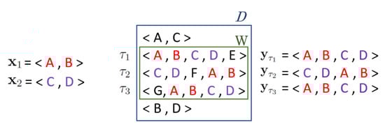
Figure 1. Graphical representation of the case $C{S}_W\left(\mathcal{D}\right)=2$. Sequences $x_1$ and $x_2$ are closed sequences in $\mathcal{D}$ with the same support set W.

Note that the previous lemma represents a sequential patterns version of Lemma 3 of Reference [5] for itemsets, where the upper bound to the number of closed itemsets in $\mathcal{D}$ with W as support set is one (this holds by the nature of the itemsets where the notion of ‘‘ordering” is not defined). Lemma 1 is crucial for proving the following lemma which provides a bound on the size of the set $V_{\mathcal{D}}$ of binary vectors.

Lemma 2

(Proof in Appendix A). $V_{\mathcal{D}}=\{v_{\mathcal{D}}\left(p\right):p\in CS\left(\mathcal{D}\right)\}\cup \left\{(0,\cdots ,0)\right\}$ and $|V_{\mathcal{D}}|\le |CS\left(\mathcal{D}\right)|+1$, that is, each vector of $V_{\mathcal{D}}$ different from $(0,\cdots ,0)$ is associated with at least one closed sequential pattern in $\mathcal{D}$.

Combining a partitioning of $CS\left(\mathcal{D}\right)$ with the previous lemma we can define a function $\tilde{w}$, an upper bound to the function w of Theorem 7, which is efficient to compute with a single scan of $\mathcal{D}$. Let $\mathcal{I}$ be the set of items that appear in the dataset $\mathcal{D}$ and ${<}_o$ be its increasing ordering by their support in $\mathcal{D}$ (ties broken arbitrarily). Given an item a, let $T_{\mathcal{D}}\left(⟨\left\{a\right\}⟩\right)$ be its support set on $\mathcal{D}$. Let ${<}_a$ denote the increasing ordering of the transactions $T_{\mathcal{D}}\left(⟨\left\{a\right\}⟩\right)$ by the number of items contained that come after a w.r.t. the ordering ${<}_o$ (ties broken arbitrarily). Let $CS\left(\mathcal{D}\right)=C_1\cup C_{2+}$, where $C_1=\{p\in CS\left(\mathcal{D}\right):|\left|p\right||=1\}$ and $C_{2+}=\{p\in CS\left(\mathcal{D}\right):|\left|p\right||\ge 2\}$. Let us focus on partitioning $C_{2+}$. Let $p\in C_{2+}$ and let a be the item in p which comes before any other item in p w.r.t. the order ${<}_o$. Let $\tau$ be the transaction containing p which comes before any other transaction containing p w.r.t. the order ${<}_a$. We assign p to the set $C_{a,\tau }$. Remember that an item can appear multiple times in a sequence. Given a transaction $\tau \in T_{\mathcal{D}}\left(⟨\left\{a\right\}⟩\right)$, $k_{a,\tau }$ is the number of items in $\tau$ (counted with their multiplicity) equal to a or that come after a in ${<}_o$. Let $m_{a,\tau }$ be the multiplicity of a in $\tau$. For each $k,m\ge 1$, $m\le k$, let $g_{a,k,m}$ be the number of transactions in $T_{\mathcal{D}}\left(⟨\left\{a\right\}⟩\right)$ that contain exactly k items (counted with their multiplicity) equal to a or located after a in the ordering ${<}_o$, with exactly m repetitions of a. Let ${\chi }_a=max\{k:g_{a,k,m}>0\}$. The following lemma gives us an upper bound to the size of $C_{a,\tau }$.

Lemma 3

(Proof in Appendix A). We have

$$|C_{a,\tau }|\le 2^{k_{a,\tau }-m_{a,\tau }}(2^{m_{a,\tau }}-1).$$

(28)

Combining the following partitioning of $CS\left(\mathcal{D}\right)$ as

$$CS\left(\mathcal{D}\right)=C_1\cup C_{2+}=C_1\cup \left(\bigcup _{a\in \mathcal{I}}\bigcup _{\tau \in T_{\mathcal{D}}\left(⟨\left\{a\right\}⟩\right)}{C}_{a,\tau }\right)$$

(29)

with the previous lemma, we obtain

$$\left|CS\left(\mathcal{D}\right)\right|\le \left|\mathcal{I}\right|+\sum _{a\in \mathcal{I}}\sum _{\tau \in T_{\mathcal{D}}\left(⟨\left\{a\right\}⟩\right)}{2}^{k_{a,\tau }-m_{a,\tau }}(2^{m_{a,\tau }}-1).$$

(30)

Now we are ready to define the function $\tilde{w}$, which can be used to obtain an efficiently computable upper bound to $R_{\mathcal{D}}$. The following lemma represents the analogous of Lemma 5 of Reference [5], adjusted for sequential patterns. Let $\overline{\eta }$ be the average item-length of the transactions of $\mathcal{D}$, that is, $\overline{\eta }={\sum }_{t\in \mathcal{D}}\left|\right|t\left|\right|/n$. Let $\widehat{\eta }$ be the maximum item-length of the transactions of $\mathcal{D}$, that is, $\widehat{\eta }={max}_{t\in \mathcal{D}}\left|\right|t\left|\right|$. Let $\eta$ be an item-length threshold, with $\overline{\eta }<\eta \le \widehat{\eta }$. Let $\mathcal{D}\left(\eta \right)$ be the bag of transactions of $\mathcal{D}$ with item-length greater than $\eta$. Let $V_{\mathcal{D}\left(\eta \right)}$ be the set of the $2^{\left|\mathcal{D}\right(\eta \left)\right|}-1$ binary vectors associated with all possible non-empty sub-bags of $\mathcal{D}\left(\eta \right)$.

Lemma 4

(Proof in Appendix A). Given an item a in $\mathcal{I}$, we define the following quantity:

$$q(a,\eta )=1+\sum _{k=1}^{{\chi }_a}\sum _{m=1}^k\sum _{j=1}^{g_{a,k,m}}\left(\mathbb{1}(k\le \eta )2^{k-m}(2^m-1)+\mathbb{1}(k>\eta )\sum _{i=1}^{\eta -1}\left(\genfrac{}{}{0pt}{}{k-1}{i}\right)\right).$$

(31)

Let $\tilde{w}:{\mathbb{R}}^{+}\to {\mathbb{R}}^{+}$ be the function

$$\tilde{w}(s,\eta )={\displaystyle \frac{1}{s}}ln\sum _{a\in \mathcal{I}}\left(q(a,\eta )e^{{\displaystyle \frac{s^2{f}_{\mathcal{D}}\left(⟨\left\{a\right\}⟩\right)}{2\left|\mathcal{D}\right|}}}+\left|V_{\mathcal{D}\left(\eta \right)}\right|e^{{\displaystyle \frac{s^2\left|\mathcal{D}\left(\eta \right)\right|}{{2\left|\mathcal{D}\right|}^2}}}+1\right).$$

(32)

Then,

$$R_{\mathcal{D}}\le \underset{s\in {\mathbb{R}}^{+},\overline{\eta }<\eta \le \widehat{\eta }}{min}\tilde{w}(s,\eta ).$$

(33)

For a given value of $\eta$, the function $\tilde{w}$ can be compute with a single scan of the dataset, since it requires to know $g_{a,k,m}$ for each $a\in \mathcal{I}$ and for each $k,m$, $1\le k\le {\chi }_a$, $1\le m\le k$. The values $\overline{\eta }$, $\widehat{\eta }$, and the support of each item and consequently the ordering ${<}_o$ are obtained during the dataset creation. Thus, it is sufficient to look at each transaction $\tau$, sorting the items ${\mathcal{I}}_{\tau }$ that appear in $\tau$ according to ${<}_o$, and, for each item of ${\mathcal{I}}_{\tau }$, keep track of its multiplicity $m_{a,\tau }$, compute $k_{a,\tau }$ and increase by one $g_{a,k_{a,\tau },m_{a,\tau }}$. Finally, since $\tilde{w}$ is convex and has first and second derivatives w.r.t. s everywhere in ${\mathbb{R}}^{+}$, its global minimum can be computed using a non-linear optimization solver. This procedure has to be repeated for each possible value of $\eta$ in $(\overline{\eta },\widehat{\eta }]$.

However, one could choose a particular schedule of values of $\eta$ to be tested, instead of taking into account each possible value, achieving a value of the function $\tilde{w}$ near to its minimum. A possible choice is to look at the restricted interval $[\overline{\eta }+{\beta }_1,min({\beta }_2,\widehat{\eta })]$, given two positive values for ${\beta }_1$ and ${\beta }_2$, instead of investigating the whole interval $(\overline{\eta },\widehat{\eta }]$. This choice is motivated by the fact that in Lemma 4 the value of $\eta$ gives us an idea of which term of the summation is dominant (the one based on closed sequential patterns or the one based on binary vectors). If $\eta$ is close to $\overline{\eta }$ then the number of binary vectors we count could be high, the dominant term is the one based on the set of binary vectors, and we expect the upper bound to be high. Instead, if $\eta$ is close to $\widehat{\eta }$ then the upper bound to the number of closed sequential patterns we count could be high, and the set of binary vectors we take into account is small. In this case, the dominant term is the one based on the closed sequential patterns, and the value of the upper bound could be high (since we count many sequential patterns with item-length greater than $\eta$ that instead would be associated with a small number of binary vectors). Thus, the best value of $\eta$ will be the one that is larger than $\overline{\eta }$ and smaller than $\widehat{\eta }$, enough to count not too many closed sequential patterns and binary vectors.

Finally, we define ComputeMaxDevRadeBound as the procedure for computing an upper bound to ${\mu }_R/2$ where, once the upper bound $R_{\mathcal{D}}^b$ to the Rademacher complexity $R_{\mathcal{D}}$ is computed using Algorithm 4, the upper bound ${\mu }_R^b/2$ to ${\mu }_R/2$ is obtained by

$${\displaystyle \frac{{\mu }_R^b}{2}}=2R_{\mathcal{D}}^b+\sqrt{{\displaystyle \frac{2ln(2/\delta )}{\left|\mathcal{D}\right|}}}.$$

(34)

The pseudo-code of the algorithm for computing the upper bound to $R_{\mathcal{D}}$ follows.

Algorithm4: RadeBound($\mathcal{D}$): algorithm for bounding the empirical Rademacher complexity of sequential patterns

4.2. Approximating the Rademacher Complexity of Sequential Patterns

The previous section presents an efficiently computable upper bound to the Rademacher of sequential patterns, which does not require any extraction of frequent sequences from a given dataset. Here we present a simple method that gives us an approximation of the Rademacher complexity of sequential patterns, which provides a tighter bound to the maximum deviation compared to the ones previously presented.

In the definition of the Rademacher complexity, a given combination $\overline{\sigma }$ of the Rademacher r.v. $\sigma$ splits the dataset $\mathcal{D}$ of n transactions in two sub-samples ${\mathcal{D}}_1\left(\overline{\sigma }\right)$ and ${\mathcal{D}}_{-1}\left(\overline{\sigma }\right)$: each transaction associated with 1 and $-1$ goes respectively into ${\mathcal{D}}_1\left(\overline{\sigma }\right)$ and ${\mathcal{D}}_{-1}\left(\overline{\sigma }\right)$. For a given sequential pattern $p\in \mathbb{U}$, let $Sup{p}_{{\mathcal{D}}_1\left(\overline{\sigma }\right)}\left(p\right)$ and $Sup{p}_{{\mathcal{D}}_{-1}\left(\overline{\sigma }\right)}\left(p\right)$ be respectively the number of transactions of ${\mathcal{D}}_1\left(\overline{\sigma }\right)$ and ${\mathcal{D}}_{-1}\left(\overline{\sigma }\right)$ in which p appears. Thus, the Rademacher complexity can be rewritten as follows:

$$R_{\mathcal{D}}={\mathbb{E}}_{\sigma }\left[\underset{p\in \mathbb{U}}{sup}{\displaystyle \frac{1}{n}}\sum _{i=1}^n{\sigma }_i{\varphi }_p\left(t_i\right)\right]={\mathbb{E}}_{\sigma }\left[\underset{p\in \mathbb{U}}{sup}{\displaystyle \frac{Sup{p}_{{\mathcal{D}}_1\left(\sigma \right)}\left(p\right)-Sup{p}_{{\mathcal{D}}_{-1}\left(\sigma \right)}\left(p\right)}{n}}\right].$$

(35)

In our approximation method we generate a single combination $\overline{\sigma }$ of the Rademacher r.v. $\sigma$, instead of generating every possible combination and then taking the expectation. Given $\overline{\sigma }$, the approximation ${\tilde{R}}_{\mathcal{D}}\left(\overline{\sigma }\right)$ of $R_{\mathcal{D}}$ is

$${\tilde{R}}_{\mathcal{D}}\left(\overline{\sigma }\right)=\underset{p\in \mathbb{U}}{sup}{\displaystyle \frac{Sup{p}_{{\mathcal{D}}_1\left(\overline{\sigma }\right)}\left(p\right)-Sup{p}_{{\mathcal{D}}_{-1}\left(\overline{\sigma }\right)}\left(p\right)}{n}}.$$

(36)

The first step of the procedure is to mine frequent sequential patterns from ${\mathcal{D}}_1\left(\overline{\sigma }\right)$ and ${\mathcal{D}}_{-1}\left(\overline{\sigma }\right)$, given a frequency threshold $\kappa$. Let $FSP({\mathcal{D}}_1\left(\overline{\sigma }\right),\kappa )$ and $FSP({\mathcal{D}}_{-1}\left(\overline{\sigma }\right),\kappa )$ be the sets of sequential patterns with support greater or equal than $\kappa$ in ${\mathcal{D}}_1\left(\overline{\sigma }\right)$ and ${\mathcal{D}}_{-1}\left(\overline{\sigma }\right)$, respectively. Let us define the following quantities:

$$\gamma \left(p\right)=Sup{p}_{{\mathcal{D}}_1\left(\overline{\sigma }\right)}\left(p\right)-Sup{p}_{{\mathcal{D}}_{-1}\left(\overline{\sigma }\right)}\left(p\right),$$

(37)

$${\gamma }_1=sup\{\gamma \left(p\right):p\in FSP({\mathcal{D}}_1\left(\overline{\sigma }\right),\kappa )\cap FSP({\mathcal{D}}_{-1}\left(\overline{\sigma }\right),\kappa )\},$$

(38)

and

$${\gamma }_2=sup\{\gamma \left(p\right):p\in FSP({\mathcal{D}}_1\left(\overline{\sigma }\right),\kappa )\setminus FSP({\mathcal{D}}_{-1}\left(\overline{\sigma }\right),\kappa )\}.$$

(39)

If $max({\gamma }_1,{\gamma }_2)/n\ge \kappa$ then ${\tilde{R}}_{\mathcal{D}}\left(\overline{\sigma }\right)=max({\gamma }_1,{\gamma }_2)/n$, since each pattern p that is not frequent in both sub-samples has $\gamma \left(p\right)/n$ lower than $\kappa$. Instead, if $max({\gamma }_1,{\gamma }_2)/n<\kappa$ the entire procedure is repeated with $\kappa =max({\gamma }_1,{\gamma }_2)/n$. Note that, since the Rademacher complexity is a non-negative quantity, it is not necessary to look at patterns in $FSP({\mathcal{D}}_{-1}\left(\overline{\sigma }\right),\kappa )\setminus FSP({\mathcal{D}}_1\left(\overline{\sigma }\right),\kappa )$ since their $\gamma \left(p\right)$’s values are negative. The pseudo-code of the method for finding an approximation of $R_{\mathcal{D}}$ is presented in Algorithm 5. The extraction of frequent sequences from the two sub-samples can be done using one of the many algorithms for mining frequent sequential patterns.

Algorithm5: RadeApprox($\mathcal{D},\kappa$): algorithm for approximating the Rademacher complexity of sequential patterns.

Finally, we define ComputeMaxDevRadeApprox as the procedure for computing an approximation of ${\mu }_R/2$ where, once the approximation $R_{\mathcal{D}}^a$ of the Rademacher complexity $R_{\mathcal{D}}$ is computed using Algorithm 5, the approximation ${\mu }_R^a/2$ of ${\mu }_R/2$ is obtained by:

$${\displaystyle \frac{{\mu }_R^a}{2}}=2R_{\mathcal{D}}^a+\sqrt{{\displaystyle \frac{2ln(2/\delta )}{\left|\mathcal{D}\right|}}}.$$

(40)

5. Sampling-Based Algorithm for Frequent Sequential Pattern Mining

We now present a sampling algorithm for frequent sequential pattern mining. The aim of this algorithm is to reduce the amount of data to consider to mine the frequent sequential patterns, in order to speed up the extraction of the sequential patterns and to reduce the amount of memory required. We define a random sample as a bag of m transactions taken uniformly and independently at random, with replacement, from $\mathcal{D}$. Obtaining the exact set $FSP(\mathcal{D},\theta )$ from a random sample is not possible, thus we focus on obtaining an $\epsilon$-approximation with probability at least $1-\delta$, where $\delta \in (0,1)$ is a confidence parameter, whose value, with $\epsilon$, is provided in input by the user. Intuitively, if a random sample is sufficiently large, then the set of frequent sequential patterns extracted from the random sample well approximates the set $FSP(\mathcal{D},\theta )$. The challenge is to find the number of transactions that are necessary to obtain the desired $\epsilon$-approximation. To compute such sample size, our approach uses the VC-dimension of sequential patterns (see Section 3.1).

Theorem 8.

Given $\epsilon ,\delta \in (0,1)$, let S be a random sample of size m sequential transactions taken independently at random with replacement from the dataset $\mathcal{D}$ such that ${sup}_{p\in \mathbb{U}}|f_{\mathcal{D}}\left(p\right)-f_S\left(p\right)|\le \epsilon /2$ with probability at least $1-\delta$. Then, given $\theta \in (0,1]$, the set $FSP(S,\theta -\epsilon /2)$ is an ε-approximation to $FSP(\mathcal{D},\theta )$ with probability at least $1-\delta$.

Proof. 

Suppose that ${sup}_{p\in \mathbb{U}}|f_{\mathcal{D}}\left(p\right)-f_S\left(p\right)|\le \epsilon /2$. In such a scenario, we have that for all sequential patterns $p\in \mathcal{D}$, it results $f_S\left(p\right)\in [f_{\mathcal{D}}\left(p\right)-\epsilon /2,f_{\mathcal{D}}\left(p\right)+\epsilon /2]$. This also holds for the sequential patterns in $\mathcal{C}=FSP(S,\theta -\epsilon /2)$. Therefore, the set $\mathcal{C}$ satisfies Property 3 from Definition 1. It also means that for all $p\in FSP(\mathcal{D},\theta )$, $f_S\left(p\right)\ge \theta -\epsilon /2$, so such $p\in \mathcal{C}$ and $\mathcal{C}$ also satisfies Property 1. Now, let $p^{*}$ be a sequential pattern such that $f_{\mathcal{D}}\left(p^{*}\right)<\theta -\epsilon$. Then, $f_S\left(p^{*}\right)<\theta -\epsilon /2$, that is $p^{*}\notin \mathcal{C}$, which allows us to conclude that $\mathcal{C}$ also has Property 2 from Definition 1. Since we know that ${sup}_{p\in \mathbb{U}}|f_{\mathcal{D}}\left(p\right)-f_S\left(p\right)|\le \epsilon /2$ with probability at least $1-\delta$, then the set $\mathcal{C}$ is an $\epsilon$-approximation to $FSP(\mathcal{D},\theta )$ with probability at least $1-\delta$, which concludes the proof. □

Theorem 8 provides a simple sampling-based algorithm to obtain an $\epsilon$-approximation to $FSP(\mathcal{D},\theta )$ with probability $\ge 1-\delta$: take a random sample of m transactions from $\mathcal{D}$ such that the maximum deviation is bounded by $\epsilon /2$, that is, ${sup}_{p\in \mathbb{U}}|f_{\mathcal{D}}\left(p\right)-f_S\left(p\right)|\le \epsilon /2$; report in output the set $FSP(S,\theta -\epsilon /2)$. As illustrated in Section 3.1, such sample size can be computed using an efficient upper bound on the VC-dimension, given in input the desired upper bound on the maximum deviation $\epsilon /2$ (see Algorithm 2). Note that such sample size can not be computed with the Rademacher complexity, since the sample size appears in both terms of the right-hand side of Equation (23). Thus, it is not possible to fix the value of the bound on the maximum deviation to compute the sample size that provides such guarantees. Algorithm 6 shows the pseudo-code of the sampling algorithm.

We now provide the respective theorem to find a FPF $\epsilon$-approximation.

Theorem 9.

Given $\epsilon ,\delta \in (0,1)$, let S be a random sample of size m sequential transactions taken independently at random with replacement from the dataset $\mathcal{D}$ such that ${sup}_{p\in \mathbb{U}}|f_{\mathcal{D}}\left(p\right)-f_S\left(p\right)|\le \epsilon /2$ with probability $\ge 1-\delta$. Then, given $\theta \in (0,1]$, the set $FSP(S,\theta +\epsilon /2)$ is a FPF ε-approximation to $FSP(\mathcal{D},\theta )$ with probability $\ge 1-\delta$.

Proof. 

Suppose that ${sup}_{p\in \mathbb{U}}|f_{\mathcal{D}}\left(p\right)-f_S\left(p\right)|\le \epsilon /2$. In such a scenario, we have that for all sequential patterns $p\in \mathcal{D}$, it results $f_S\left(p\right)\in [f_{\mathcal{D}}\left(p\right)-\epsilon /2,f_{\mathcal{D}}\left(p\right)+\epsilon /2]$. This also holds for the sequential patterns in $\mathcal{F}=FSP(S,\theta +\epsilon /2)$. Therefore, the set $\mathcal{F}$ satisfies Property 3 from Definition 2. It also means that for all $p^{*}\notin FSP(\mathcal{D},\theta )$, $f_S\left(p^{*}\right)<\theta +\epsilon /2$, so such $p^{*}\notin \mathcal{F}$ and $\mathcal{F}$ also satisfies Property 1. Now, let $p^{\prime }$ be a sequential pattern such that $f_{\mathcal{D}}\left(p^{\prime }\right)\ge \theta +\epsilon$. Then, $f_S\left(p^{\prime }\right)\ge \theta +\epsilon /2$, that is $p^{\prime }\in \mathcal{F}$, which allows us to conclude that $\mathcal{F}$ also has Property 2 from Definition 2. Since we know that ${sup}_{p\in \mathbb{U}}|f_{\mathcal{D}}\left(p\right)-f_S\left(p\right)|\le \epsilon /2$ with probability at least $1-\delta$, then the set $\mathcal{F}$ is a FPF $\epsilon$-approximation to $FSP(\mathcal{D},\theta )$ with probability at least $1-\delta$, which concludes the proof. □

Algorithm6: Sampling-Based Algorithm for Frequent Sequential Pattern Mining.

Data: Dataset $\mathcal{D}$; $\epsilon ,\delta \in (0,1)$; $\theta \in (0,1]$.    Result: Set $\mathcal{C}$ that is an $\epsilon$-approximation (resp. a FPF $\epsilon$-approximation) to $FSP(\mathcal{D},\theta )$ with probability $\ge 1-\delta$. 1 $m\leftarrow$ ComputeSampleSize($\mathcal{D},\epsilon ,\delta )$ 2 $S\leftarrow$ sample of m transactions taken independently at random with replacement from $\mathcal{D}$; 3 $\mathcal{C}\leftarrow FSP(S,\theta -\epsilon /2)$; /* resp. $\theta +\epsilon /2$ to obtain a FPF $\epsilon$-approximation */ 4 return$\mathcal{C}$;

As explained above, the sample size m can be computed with Algorithm 2 that uses an efficient upper bound on the VC-dimension of sequential patterns. Then, the sample is generated taking m transactions uniformly and independently at random, with replacement, from $\mathcal{D}$. Finally, the mining of the sample S can be performed with any efficient algorithm for the exact mining of frequent sequential patterns. Figure 2 depicts a block diagram representing the relations between the algorithms presented in this work.

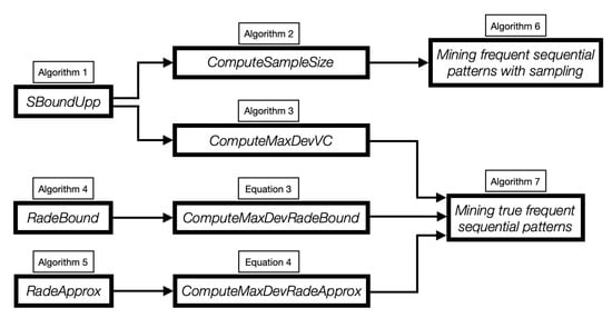
Figure 2. Block diagram representing the relations between our algorithms.

6. Algorithms for True Frequent Sequential Pattern Mining

In this section, we describe our approach to find rigorous approximations to the TFSPs. In particular, given a dataset $\mathcal{D}$, that is a finite bag of $\left|\mathcal{D}\right|$ i.i.d. samples from an unknown probability distribution $\pi$ on $\mathbb{U}$, a minimum frequency threshold $\theta$ and a confidence parameter $\delta$, we aim to find rigorous approximations of the TFSPs w.r.t. $\theta$, defined in Definitions 3 and 4, with probability at least $1-\delta$.

The intuition behind our approach is the following. If we know an upper bound $\mu /2$ on the maximum deviation, that is ${sup}_{p\in \mathbb{U}}|t_{\pi }\left(p\right)-f_{\mathcal{D}}\left(p\right)|\le \mu /2$, we can identify a frequency threshold $\widehat{\theta }$ (resp. $\tilde{\theta }$) such that the set $FSP(\mathcal{D},\widehat{\theta })$ is a FPF $\mu$-approximation (resp. $FSP(\mathcal{D},\tilde{\theta })$ is a $\mu$-approximation) of $TFSP(\pi ,\theta )$. The upper bound on the maximum deviation can be computed, as illustrated in the previous sections, with the empirical VC-dimension and with the Rademacher complexity.

We now describe how to identify the threshold $\widehat{\theta }$ that allows to obtain a FPF $\mu$-approximation. Suppose that ${sup}_{p\in \mathbb{U}}|t_{\pi }\left(p\right)-f_{\mathcal{D}}\left(p\right)|\le \mu /2$. In such a scenario, we have that every sequential pattern $p^{*}\notin TFSP(\pi ,\theta )$, and so that has $t_{\pi }\left(p^{*}\right)<\theta$, has a frequency $f_{\mathcal{D}}\left(p^{*}\right)<\theta +\mu /2=\widehat{\theta }$. Hence, the only sequential patterns that can have frequency in $\mathcal{D}$ greater or equal to $\widehat{\theta }=\theta +\mu /2$, are those with true frequency at least $\theta$. The intuition is that if we find a $\mu$ such that ${sup}_{p\in \mathbb{U}}|t_{\pi }\left(p\right)-f_{\mathcal{D}}\left(p\right)|\le \mu /2$, we know that all the sequences $p\in \mathbb{U}$, that are not true frequent w.r.t $\theta$, can not be in $FSP(\mathcal{D},\widehat{\theta })$. The following theorem formalizes the strategy to obtain a FPF $\mu$-approximation. Algorithm 7 shows the pseudo-code to mine the true frequent sequential patterns.

Theorem 10 shows how to compute a corrected threshold $\widehat{\theta }$ such that the set $FSP(D,\widehat{\theta })$ is a FPF $\mu$-approximation of $TFSP(\pi ,\theta )$, that is, $FSP(D,\widehat{\theta })$ only contains sequential patterns that are in $TFSP(\pi ,\theta )$. It guarantees that with high probability the set $FSP(\mathcal{D},\widehat{\theta })$ does not contain false positives but it has not guarantees on the number of false negatives, that is, sequential patterns that are in $TFSP(\pi ,\theta )$ but not in $FSP(\mathcal{D},\widehat{\theta })$. On the other hand, we might be interested in finding all the true frequent sequential patterns in $TFSP(\pi ,\theta )$. The following result shows how to identify a threshold $\tilde{\theta }$ such that the set $FSP(\mathcal{D},\tilde{\theta })$ contains all the true frequent sequential patterns in $TFSP(\pi ,\theta )$ with high probability, that is, $FSP(\mathcal{D},\tilde{\theta })$ is a $\mu$-approximation of $TFSP(\pi ,\theta )$. Note that while Theorem 11 provides guarantees on false negatives, it does not provide guarantees on the number of false positives in $FSP(\mathcal{D},\tilde{\theta })$.

Algorithm 7 shows the pseudo-code of the two strategies to mine the true frequent sequential patterns. To compute an upper bound on the maximum deviation, it is possible to use Algorithm 3 based on the empirical VC-dimension or the two procedures ComputeMaxDevRadeBound (Equation (34)) and ComputeMaxDevRadeApprox (Equation (40)) based on the Rademacher complexity. The mining of $\mathcal{D}$ can be performed with any efficient algorithm for the exact mining of frequent sequential patterns. Figure 2 shows the relations between the algorithms we presented for mining true frequent sequential patterns.

Theorem 10.

Given $\delta \in (0,1)$, such that ${sup}_{p\in \mathbb{U}}|t_{\pi }\left(p\right)-f_{\mathcal{D}}\left(p\right)|\le \mu /2$ with probability at least $1-\delta$, and given $\theta \in (0,1]$, the set $FSP(\mathcal{D},\widehat{\theta })$, with $\widehat{\theta }=\theta +\mu /2$, is a FPF μ-approximation of the set $TFSP(\pi ,\theta )$ with probability at least $1-\delta$.

Proof. 

Suppose that ${sup}_{p\in \mathbb{U}}|t_{\pi }\left(p\right)-f_{\mathcal{D}}\left(p\right)|\le \mu /2$. Thus, we have that for all the sequential patterns $p\in \mathbb{U}$, it results $f_{\mathcal{D}}\left(p\right)\in [t_{\pi }\left(p\right)-\mu /2,t_{\pi }\left(p\right)+\mu /2]$. This also holds for the sequential patterns in $\mathcal{G}=FSP(\mathcal{D},\widehat{\theta })$. Therefore, the set $\mathcal{G}$ satisfies Property 3 of Definition 4. Let $p^{*}$ be a sequential pattern such that $t_{\pi }\left(p^{*}\right)<\theta$, that is, it is not a true frequent sequential pattern w.r.t. $\theta$. Then, $f_{\mathcal{D}}\left(p^{*}\right)<\theta +\mu /2=\widehat{\theta }$, that is, $p^{*}\notin \mathcal{G}$, which allows us to conclude that $\mathcal{G}$ also has Property 1 from Definition 4. Now, let $p^{\prime }$ be a sequential pattern such that $t_{\pi }\left(p^{\prime }\right)\ge \theta +\mu$. Then, $f_{\mathcal{D}}\left(p^{\prime }\right)\ge \theta +\mu /2$, that is $p^{\prime }\in \mathcal{G}$, which allows us to conclude that $\mathcal{G}$ also has Property 2 from Definition 4. Since we know that ${sup}_{p\in \mathbb{U}}|t_{\pi }\left(p\right)-f_{\mathcal{D}}\left(p\right)|\le \mu /2$ with probability at least $1-\delta$, then the set $\mathcal{G}$ is a FPF $\mu$-approximation of $TFSP(\pi ,\theta )$ with probability at least $1-\delta$, which concludes the proof. □

Theorem 11.

Given $\delta \in (0,1)$, such that ${sup}_{p\in \mathbb{U}}|t_{\pi }\left(p\right)-f_{\mathcal{D}}\left(p\right)|\le \mu /2$ with probability at least $1-\delta$, and given $\theta \in (0,1]$, the set $FSP(\mathcal{D},\tilde{\theta })$, with $\tilde{\theta }=\theta -\mu /2$, is a μ-approximation of the set $TFSP(\pi ,\theta )$ with probability at least $1-\delta$.

Proof. 

Suppose that ${sup}_{p\in \mathbb{U}}|t_{\pi }\left(p\right)-f_{\mathcal{D}}\left(p\right)|\le \mu /2$. Thus, we have that for all the sequential patterns $p\in \mathbb{U}$, it results $f_{\mathcal{D}}\left(p\right)\in [t_{\pi }\left(p\right)-\mu /2,t_{\pi }\left(p\right)+\mu /2]$. This also holds for the sequential patterns in $\mathcal{E}=FSP(\mathcal{D},\tilde{\theta })$. Therefore, the set $\mathcal{E}$ satisfies Property 3 of Definition 3. It also means that for all $p\in TFSP(\pi ,\theta )$, $f_{\mathcal{D}}\left(p\right)\ge \theta -\mu /2=\tilde{\theta }$, that is, $p\in \mathcal{E}$, which allows us to conclude that $\mathcal{E}$ also has Property 1 from Definition 3. Now, let $p^{*}$ be a sequential pattern such that $t_{\pi }\left(p^{*}\right)<\theta -\mu$. Then, $f_{\mathcal{D}}\left(p^{*}\right)<\theta -\mu /2$, that is $p^{*}\notin \mathcal{E}$, which allows us to conclude that $\mathcal{E}$ also has Property 2 from Definition 3. Since we know that ${sup}_{p\in \mathbb{U}}|t_{\pi }\left(p\right)-f_{\mathcal{D}}\left(p\right)|\le \mu /2$ with probability at least $1-\delta$, then the set $\mathcal{E}$ is a $\mu$-approximation of $TFSP(\pi ,\theta )$ with probability at least $1-\delta$, which concludes the proof. □

Algorithm7: Mining the True Frequent Sequential Patterns.

Data: Dataset $\mathcal{D}$; $\delta \in (0,1)$; $\theta \in (0,1]$    Result: Set $\mathcal{G}$ that is a FPF $\mu$-approximation (resp. $\mu$-approximation) to $TFSP(\pi ,\theta )$ with probability $\ge 1-\delta$. 1 $\mu /2\leftarrow$ ComputeMaxDeviationBound($\mathcal{D},\delta$); 2 $\mathcal{G}\leftarrow FSP(\mathcal{D},\theta +\mu /2)$; /* resp. $\theta -\mu /2$ to obtain a $\mu$-approximation */ 3 return$\mathcal{P}$;

7. Experimental Evaluation

In this section, we report the results of our experimental evaluation on multiple datasets to assess the performance of the algorithms we proposed in this work. The goals of the evaluation are the following:

• Assess the performance of our sampling algorithm. In particular, to asses whether with probability $1-\delta$ the sets of frequent sequential patterns extracted from samples are $\epsilon$-approximations, for the first strategy, and FPF $\epsilon$-approximations, for the second one, of $FSP(\mathcal{D},\theta )$. In addition, we compared the performance of the sampling algorithm with the ones to mine the full datasets in term of execution time.
• Assess the performance of our algorithms for mining the true frequent sequential patterns. In particular, to assess whether with probability $1-\delta$ the set of frequent sequential patterns extracted from the dataset with the corrected threshold does not contain false positives, that is, it is a FPF $\mu$-approximation of $TSFP(\pi ,\theta )$, for the first method, and contains all the TFSPs, that is, it is a $\mu$-approximation of $TSFP(\pi ,\theta )$, for the second method. In addition, we compared the results obtained with the VC-dimension and with the Rademacher complexity, both used to compute an upper bound on the maximum deviation.

Since no sampling algorithm for rigorously approximating the set of frequent sequential patterns and no algorithm to mine true frequent sequential patterns have been previously proposed, we do not consider other methods in our experimental evaluation.

7.1. Implementation and Environment

The code to compute the bound on the VC-dimension (Algorithm 1) and to perform the evaluation has been developed in Java and executed using version 1.8.0_201. The code to compute the bound and the approximation to the Rademacher Complexity (resp. Algorithms 4 and 5) has been developed in C++. We have performed all our experiments on the same machine with 512 GB of RAM and 2 Intel(R) Xeon(R) CPU E5-2698 v3 @ 2.3GHz. To mine sequential patterns, we used the PrefixSpan [10] implementation provided by the SPMF library [28]. We used NLopt [29] as non-linear optimization solver. Our open-source implementation and the code developed for the tests, including scripts to reproduce all results, are available online [30].

7.2. Datasets

In this section, we describe the datasets we used in our evaluation. We first describe the dataset used to evaluate our sampling algorithm for FSP mining, and then the datasets used for TFSP mining. All datasets are obtained starting from the following real datasets:

• BIBLE: a conversion of the Bible into sequence where each word is an item;
• BMS1: contains sequences of click-stream data from the e-commerce website Gazelle;
• BMS2: contains sequences of click-stream data from the e-commerce website Gazelle;
• FIFA: contains sequences of click-stream data from the website of FIFA World Cup 98;
• KOSARAK: contains sequences of click-stream data from an Hungarian news portal;
• LEVIATHAN: is a conversion of the novel Leviathan by Thomas Hobbes (1651) as a sequence dataset where each word is an item;
• MSNBC: contains sequences of click-stream data from MSNBC website and each item represents the category of a web page;
• SIGN: contains sign language utterance.

All the datasets used are publicly available online [31] and the code to generate the pseudo-artificial datasets, as described in the following sections, is provided [30]. The characteristics of the datasets are reported in Table 1.

Table 1. Datasets characteristics. For each dataset $\mathcal{D}$, we report the number $\left|\mathcal{D}\right|$ of transactions, the total number $\left|\mathcal{I}\right|$ of items, the average transaction item-length and the maximum transaction item-length.

Dataset $\mathcal{D}$	Size $\left|\mathcal{D}\right|$	$\left|\mathcal{I}\right|$	Avg. Item-Length	Max. Item-Length
BIBLE	36,369	13,905	21.6	100
BMS1	59,601	497	2.5	267
BMS2	77,512	3340	4.6	161
FIFA	20,450	2990	36.2	100
KOSARAK	69,999	14,804	8.0	796
LEVIATHAN	5835	9025	33.8	100
MSNBC	989,818	17	4.8	14,795
SIGN	730	267	52.0	94

7.2.1. FSP Mining

The typical scenario for the application of sampling is that the dataset to mine is very large, sometimes even too large to fit in the main memory of the machine. Thus, in applying sampling techniques, we aim to reduce the size of such dataset, considering only a sample of it, in order to obtain an amount of data of reasonable size. Since the number of transactions in each real dataset (shown in Table 1) is fairly limited, we replicated each dataset to reach modern datasets sizes. For each real dataset, we fixed a replication factor and we created a new dataset, replicating each transaction in the dataset a number of times equal to the replication factor. Then, the input data for the sampling algorithm is the new enlarged dataset. The replication factors used are the following: BIBLE and FIFA = 200x; BMS1, BMS2 and KOSARAK = 100x; LEVIATHAN = 1000x; MSNBC = 10x and SIGN = 10,000x.

7.2.2. TFSP Mining

To evaluate our algorithms to mine the true frequent sequential patterns, we need to know which are the sequential patterns that are frequently generated from the unknown generative process $\pi$. In particular, we need a ground truth of the true frequencies of the sequential patterns. We generated pseudo-artificial datasets by taking some of the datasets in Table 1 as ground truth for the true frequencies $t_{\pi }$ of the sequential patterns. For each ground truth, we created four new datasets by sampling sequential transactions uniformly at random from the original dataset. All the new datasets have the same number of transactions of the respectively ground truth, that is, the respectively original dataset. We used the original datasets as ground truth and we executed our evaluation in the new (sampled) datasets. Therefore, the true frequency of a sequential pattern is its frequency in the original dataset, that is, its frequency in the original dataset is exactly the same that such pattern would have in an hypothetical infinite number of transactions generated by the unknown generative process $\pi$.

7.3. Sampling Algorithm Results

In this section, we describe the results obtained with our sampling algorithm (Algorithm 6). As explained above, the typical scenario to apply sampling is that the dataset to mine is very large. Thus, we aim to reduce the size of such dataset, considering only a sample of it. In addition, from the sample, we aim to obtain a good approximation of the results that would have been obtained from the entire dataset. In all our experiments we fixed $\epsilon =0.01$ and $\delta =0.1$. The steps of the evaluation are the following (Algorithm 6): given a dataset ${\mathcal{D}}_L$ as input, we compute the sample size m, using Algorithm 2, to obtain an $\epsilon =0.01$-approximation (resp. FPF $0.01$-approximation) with probability at least $1-\delta =0.90$. Then, we extract a random sample S of m transactions from ${\mathcal{D}}_L$ and we run the algorithm to mine the frequent sequential patterns on S. Finally, we verify whether the set of frequent sequential patterns extracted from the sample is a $0.01$-approximation (resp. FPS $0.01$-approximation) to $FSP({\mathcal{D}}_L,\theta )$. For each dataset ${\mathcal{D}}_L$ we repeat the experiment 5 times, and then we compute the fraction of times the sets of frequent sequential patterns extracted from the samples have the properties described in Definition 1 (resp. Definition 2). Table 2 shows the results.

Table 2. Sampling algorithms results. For each enlarged dataset ${\mathcal{D}}_L$, we report $\theta$, the ratio $\left|S\right|/|{\mathcal{D}}_L|$ between the sample size $\left|S\right|$ and the size of the enlarged dataset $|{\mathcal{D}}_L|$, Max_Abs_Err, the maximum ${max}_{p\in C_i}|f_{\mathcal{D}}\left(p\right)-f_{S_i}\left(p\right)|$, and Avg_Abs_Err, the average ${max}_{p\in C_i}|f_{\mathcal{D}}\left(p\right)-f_{S_i}\left(p\right)|$, over the 5 samples $S_i$ and with $C_i$ the set of frequent sequential patterns extracted from $S_i$, the percentage of $\epsilon$-approximations obtained over the 5 samples and the percentage of FPF $\epsilon$-approximations obtained over the 5 samples.

Dataset ${\mathcal{D}}_{\mathit{L}}$	$\mathit{\theta }$	$\left|\mathit{S}\right|/|{\mathcal{D}}_{\mathit{L}}|$	Max_Abs_Err (×${10}^{-4})$	Avg_Abs_Err (×${10}^{-4})$	$\mathit{\epsilon }$-approx (%)	FPF $\mathit{\epsilon }$-approx (%)
BIBLE	0.1	0.24	9.33	7.47	100	100
BMS1	0.012	0.17	5.45	4.70	100	100
BMS2	0.012	0.16	4.08	3.14	100	100
FIFA	0.25	0.50	8.68	7.07	100	100
KOSARAK	0.02	0.52	7.18	4.95	100	100
LEVIATHAN	0.15	0.30	9.19	7.84	100	100
MSNBC	0.02	0.37	4.33	3.63	100	100
SIGN	0.4	0.20	14.14	12.19	100	100

We observe that the samples obtained from the datasets are about 2 to 5 times smaller than the whole datasets. Moreover, in all the runs for all the datasets, we obtain an $\epsilon$-approximation (resp. FPF $\epsilon$-approximation). Such results are even better than the theoretical guarantees, that ensure to obtain such approximations with probability at least 90%. We also reported Max_Abs_Err $={max}_{S_i,i\in [1,5]}{max}_{p\in C_i}|f_{\mathcal{D}}\left(p\right)-f_{S_i}\left(p\right)|$ and Avg_Abs_Err $=\frac{1}{5}{\sum }_{S_i,i\in [1,5]}{max}_{p\in C_i}|f_{\mathcal{D}}\left(p\right)-f_{S_i}\left(p\right)|$, where $C_i$ is the set of frequent sequential patterns extracted from the sample $S_i$, $i=1,...,5$ (since we run each experiment 5 times, there are 5 samples). They represent the maximum and the average, over the 5 runs, of the maximum absolute difference between the frequency that the sequential patterns have in the entire dataset and that they have in the sample, over all the sequential patterns extracted from the sample. Again, the results obtained are better than the theoretical guarantees, that ensure a maximal absolute difference lower than $\epsilon /2=0.005$.

Figure 3 shows the comparison between the average execution time of the sampling algorithm and the average execution time of the mining of the entire dataset, over the 5 runs. For all the datasets, the sampling algorithm requires less time than the mining of the whole dataset. For BMS1 and BMS2, the mining of the whole dataset is very fast since the number of frequent sequential patterns extracted from it is low. Thus, there is not a large difference between the execution time to mine the whole dataset and the execution time for the sampling algorithm, which is most due to the computation of the sample size. Similar results between our sampling algorithm and the mining of the whole dataset have also been obtained with KOSARAK and MSNBC. As expected, for all the datasets, the execution time of the sampling algorithm to obtain an $\epsilon$-approximation is larger than the execution time of the sampling algorithm to obtain a FPF $\epsilon$-approximation, since the minimum frequency threshold used in the first case is lower, resulting in a higher number of extracted sequential patterns.

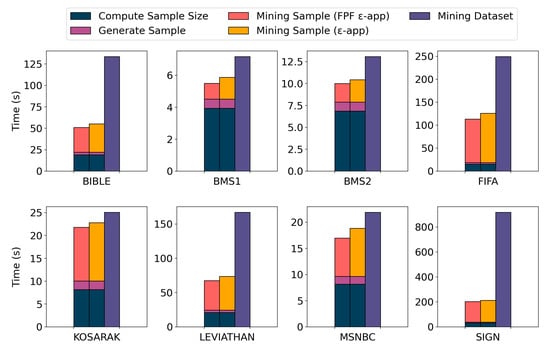
Figure 3. Execution time of the sampling algorithm. The execution time required to mine the whole dataset, and the execution times of the sampling algorithm to obtain an $\epsilon$-approximation and a false positives free (FPF) $\epsilon$-approximation are reported. For the sampling algorithms, we show the execution time to compute the sample size, the execution time to generate the sample, and the execution time to mine the sample.

We now discuss some of the patterns extracted from the MSNBC dataset, for which richer information regarding the data is available. In particular, in MSNBC each transaction contains the sequence of click-stream data generated by a single view on the MSNBC website by a user, and each item represents the category of a visited webpage, such “frontpage”, “news”, “sports”, and so forth.

The two most frequent sequential patterns extracted in the enlarged datasets with a classic FSP algorithm are single categories, that is, sequential patterns of item-length 1: $⟨\left\{frontpage\right\}⟩$ is the most frequent while $⟨\{on-air\}⟩$ is the second one. They are also the two most frequent sequential patterns extracted in all the five samples using our sampling algorithms. The most frequent sequential patterns with item-length greater than one are the sequential patterns $⟨\left\{frontpage\right\},\left\{frontpage\right\}⟩$ and $⟨\left\{frontpage\right\},\left\{frontpage\right\},\left\{frontpage\right\}⟩$. For $⟨\left\{frontpage\right\},\left\{frontpage\right\}⟩$, 75% of the transactions in which it appears there is at least an instance of such pattern where the two items are consecutive. This means that users visited two consecutive webpages of the same category, “frontpage”, or that they refreshed the same page twice, while in the 25% of the transactions in which it appears users visited webpages of other categories between the two “frontpage” webpages. Instead, for $⟨\left\{frontpage\right\},\left\{frontpage\right\},\left\{frontpage\right\}⟩$ the percentage of transactions in which the three items are consecutive is 59%. We also observed similar results with other categories: sequential patterns that are sequences of the same item, and so of the same category, have higher frequency. This fact highlights that users usually visit more frequently pages of the same category or that they refresh multiple times the same pages.

The most frequent sequential patterns that are not sequences of the same item are combinations of the items “frontpage” and “news”, for example, $⟨\left\{frontpage\right\},\left\{news\right\}⟩$, $⟨\left\{frontpage\right\},\left\{news\right\},\left\{news\right\}⟩$ and $⟨\left\{news\right\},\left\{frontpage\right\}⟩$. Surprisingly, the item “on-air” alone is more frequent that the item “news” alone. This means that users visit “news” webpages coming from a “frontpage” more frequently than “on-air” webpages, though they visit more frequently “on-air” webpages.

7.4. True Frequent Sequential Patterns Results

In this section, we describe the results of our algorithms for mining the true frequent sequential patterns. In all these experiments, we fixed $\delta =0.1$. First of all, for each real dataset we generated 4 pseudo-artificial datasets ${\mathcal{D}}_i$, $i\in [1,4]$ from the same ground truth. We mined the set $FSP({\mathcal{D}}_i,\theta )$, and we compared it with the TFSPs, that is, the set $FSP(\mathcal{D},\theta )$, where $\mathcal{D}$ is the ground truth. Such experiments aim to verify whether the sets of the FSPs extracted from the pseudo-artificial datasets contain false positives and miss some TFSPs. Table 3 shows the fractions of times that the set $FSP({\mathcal{D}}_i,\theta )$ contains false positives and misses TFSPs from the ground truth. We ran this evaluation over the four datasets ${\mathcal{D}}_i$, $i\in [1,4]$, of the same size from the same ground truth and we reported the average. For each dataset, we report the results with two frequency thresholds $\theta$. In almost all the cases, the FSPs mined from the pseudo-artificial datasets contain false positives and miss some TFSPs. In particular, with lower frequency thresholds (and, therefore, a larger number of patterns), the fraction of times we find false positives and false negatives usually increases. These results emphasize that, in general, the mining of the FSPs is not enough to learn interesting features of the underlying generative process of the data, and techniques like the ones introduced in this work are necessary.

Table 3. Average fraction of times that $FSP({\mathcal{D}}_i,\theta )$, with ${\mathcal{D}}_i$ a pseudo-artificial dataset, contains false positives, Times FPs, and misses true frequent sequential patterns (TFSPs) (false negatives), Times FNs, over 4 datasets ${\mathcal{D}}_i$ from the same ground truth.

Ground Truth	$\mathit{\theta }$	|TFSP|	Times FPs	Times FNs
BIBLE	0.1	174	50%	100%
	0.05	774	100%	100%
BMS1	0.025	13	50%	0%
	0.0225	17	0%	25%
BMS2	0.025	10	0%	0%
	0.0225	11	0%	0%
KOSARAK	0.06	23	100%	0%
	0.04	41	50%	25%
LEVIATHAN	0.15	225	75%	100%
	0.1	651	100%	100%
MSNBC	0.02	97	75%	25%
	0.015	143	100%	50%

Then, we compute and compare the upper bounds to the maximum deviation introduced in the previous sections, since our strategy to find an approximation to the true frequent sequential patterns hinges on finding a tight upper bound to the maximum deviation. For each pseudo-artificial dataset, we computed the upper bound ${\mu }_{VC}/2$ to the maximum deviation using the VC-dimension based bound (ComputeMaxDevVC, Algorithm 3), the Rademacher complexity based bound ${\mu }_R^b/2$ (ComputeMaxDevRadeBound, Equation (34)), and the Rademacher complexity approximation ${\mu }_R^a/2$ (ComputeMaxDevRadeApprox, Equation (40)). Table 4 shows that the two methods for computing the upper bound to the maximum deviation using an upper to the empirical VC-dimension and Rademacher complexity are similar for BMS1 and BMS2, but for the other samples the VC-dimension-based algorithm is better than the one based on the Rademacher complexity bound by a factor between 2 and 3, that is, ${\mu }_R^b/{\mu }_{VC}\in [2,3]$. Tighter upper bounds to the maximum deviation are provided by the method that uses the approximation of the Rademacher complexity.

Table 4. Comparison of the upper bound $\mu /2$ to the maximum deviation achieved respectively by ComputeMaxDevVC, ComputeMaxDevRadeBound, and ComputeMaxDevRadeApprox for each dataset. We show averages $avg$, maximum values $max$, and standard deviations $std$ for each dataset and method over the 4 pseudo-artificial datasets.

Dataset	${\mathit{\mu }}_{\mathbf{VC}}/2$			${\mathit{\mu }}_{\mathit{R}}^{\mathit{b}}/2$			${\mathit{\mu }}_{\mathit{R}}^{\mathit{a}}/2$
	avg	max	std (×${10}^{-3}$)	avg	max	std (×${10}^{-3}$)	avg	max	std (×${10}^{-3}$)
BIBLE	0.0339	0.0340	0.1	0.0747	0.0748	0.1	0.0207	0.0223	1.5
BMS1	0.0194	0.0197	0.3	0.0287	0.0294	0.6	0.0136	0.0153	1.0
BMS2	0.0194	0.0196	0.1	0.0202	0.0207	0.5	0.0107	0.0115	0.5
KOSARAK	0.0334	0.0335	0.1	0.0957	0.0972	1.5	0.0145	0.0164	1.5
LEVIATHAN	0.0847	0.0850	0.3	0.1878	0.1904	1.6	0.0569	0.0636	5.5
MSNBC	0.0089	0.0090	0.1	0.0252	0.0257	0.9	0.0035	0.0041	0.4

In our implementation of Algorithm 4 to compute an upper bound to the empirical Rademacher complexity of sequential patterns, we compute several upper bounds associated with different integer values of $\eta \in [\overline{\eta }+{\beta }_1,min({\beta }_2,\widehat{\eta })]$ for fixed values of ${\beta }_1$ and ${\beta }_2$, taking the minimum bound among those computed. In our experiments, we fixed ${\beta }_1=20$ and ${\beta }_2=120$. In practice, by increasing the value of $\eta$ we observe a decreasing trend of the upper bound value until a minimum value is reached. Then, by increasing again the value of $\eta$ the value of the upper bound increases until it converges to the one achieved with $\eta =\widehat{\eta }$. In addition, for each pseudo-artificial dataset the value of $\eta$ associated with the minimum value of the upper bound to the maximum deviation is always found in $[\overline{\eta }+{\beta }_1,min({\beta }_2,\widehat{\eta })]$, with ${\beta }_1=20$, ${\beta }_2=120$.

Finally, we evaluated the performance of our two strategies to mine an approximation of the true frequent sequential patterns, the first one with guarantees on the false positives and the second one with guarantees on the false negatives, using the upper bounds on the maximum deviation computed above. We considered the two tightest upper bounds, that are ${\mu }_{VC}/2$ and ${\mu }_R^a/2$, computed respectively using the empirical VC-dimension and an approximation of the empirical Rademacher complexity. From each pseudo-artificial dataset, we mined the FSPs using $\widehat{\theta }$, for the first strategy, and $\tilde{\theta }$, for the second one, respectively computed using Theorems 10 and 11, and we compared the sequential patterns extracted with the TFSPs from the ground truth. Table 5 shows the results for the strategy with guarantees on the false positives. Using ${\mu }_{VC}/2$ to compute the corrected frequency threshold ${\widehat{\theta }}_{VC}$, our algorithm performs better than the theoretical guarantees in all the runs, since the number of times the output contains false positives is always equal to zero, while the theory guarantees a probability of at least $1-\delta =0.9$ to obtain the correct approximation. Obviously, this also happens using ${\mu }_R^a/2$ to compute the corrected frequency threshold ${\widehat{\theta }}_R$, since ${\mu }_{VC}>{\mu }_R^a$. We also computed the average fraction of TFSPs reported in the output by the algorithm, that is, $\left|FSP\right({\mathcal{D}}_i,\widehat{\theta }\left)\right|/\left|TFSP\right|$, since we aim to obtain as many TFSPs as possible. For all the datasets, it is possible to notice that the results obtained with the Rademacher complexity are better than the ones obtained with the VC-dimension, since the Rademacher allows to obtain a higher percentage of TFSPs in output. Table 6 shows the results for the strategy with guarantees on the false negatives. Similar to the previous case, our algorithm performs better than the theoretical guarantees in all the runs, since the number of times the algorithm misses some TFSPs is always equal to zero, with both the VC-dimension and the Rademacher complexity based results. We also report the average fractions of patterns in the output that are TFSPs, that is, $\left|TFSP\right|/\left|FSP\right({\mathcal{D}}_i,\tilde{\theta }\left)\right|$, since we are interested in obtaining all the TFSPs but with less false positives as possible. Again, the results with the Rademacher complexity are better than the ones obtained with the VC-dimension, since the number of sequential patterns in the output of the algorithm that are TFSPs is higher using the Rademacher complexity.

Table 5. Results of our algorithm for the TFSPs with guarantees on the false positives in 4 pseudo-artificial datasets ${\mathcal{D}}_i$ for each ground truth. The table reports the frequency thresholds $\theta$ used in the experiments, the number of TFSPs in the ground truth, the number of times the output contains false positives using ${\widehat{\theta }}_{VC}=\theta +{\mu }_{VC}/2$ as frequency threshold and the average fraction of the reported TFSPs in the output using such frequency threshold, the number of times the output contains false positives using ${\widehat{\theta }}_R=\theta +{\mu }_R^a/2$ and the average fraction of the reported TFSPs in the output using such frequency threshold.

Ground Truth	$\mathit{\theta }$	|TFSP|	Times FPs in FSP(${\mathcal{D}}_{\mathit{i}},{\widehat{\mathit{\theta }}}_{\mathbf{VC}}$)	|FSP(${\mathcal{D}}_{\mathit{i}},{\widehat{\mathit{\theta }}}_{\mathbf{VC}}\left)\right|$/ |TFSP|	Times FPs in FSP(${\mathcal{D}}_{\mathit{i}},{\widehat{\mathit{\theta }}}_{\mathit{R}}$)	|FSP(${\mathcal{D}}_{\mathit{i}},{\widehat{\mathit{\theta }}}_{\mathit{R}}\left)\right|$/ |TFSP|
BIBLE	0.1	174	0 %	0.55	0 %	0.68
	0.05	774	0 %	0.32	0 %	0.47
BMS1	0.025	13	0 %	0.38	0 %	0.48
	0.0025	17	0 %	0.29	0 %	0.43
BMS2	0.025	10	0 %	0.13	0 %	0.20
	0.0025	11	0 %	0.18	0 %	0.18
KOSARAK	0.06	23	0 %	0.41	0 %	0.73
	0.04	41	0 %	0.43	0 %	0.74
LEVIATHAN	0.15	225	0 %	0.30	0 %	0.41
	0.1	651	0 %	0.18	0 %	0.30
MSNBC	0.02	97	0 %	0.56	0 %	0.77
	0.015	143	0 %	0.50	0 %	0.76

Table 6. Results of our algorithm for the TFSPs with guarantees on the false negatives in 4 pseudo-artificial datasets ${\mathcal{D}}_i$ for each ground truth. The table reports the frequency thresholds $\theta$ used in the experiments, the number of TFSPs in the ground truth, the number of times the output of the algorithm misses some TFSPs using ${\tilde{\theta }}_{VC}=\theta -{\mu }_{VC}/2$ as frequency threshold and the average fraction of sequential patterns that are TFSPs in the output using such frequency threshold, the number of times the output of the algorithm misses some TFSPs using ${\tilde{\theta }}_R=\theta -{\mu }_R^a/2$ and the average fraction of sequential patterns that are TFSPs in the output using such frequency threshold.

Ground Truth	$\mathit{\theta }$	|TFSP|	Times FNs in FSP(${\mathcal{D}}_{\mathit{i}},{\tilde{\mathit{\theta }}}_{\mathbf{VC}}$)	|TFSP|/ |FSP(${\mathcal{D}}_{\mathit{i}},{\tilde{\mathit{\theta }}}_{\mathbf{VC}}\left)\right|$	Times FNs in FSP(${\mathcal{D}}_{\mathit{i}},{\tilde{\mathit{\theta }}}_{\mathit{R}}$)	|TFSP|/ |FSP(${\mathcal{D}}_{\mathit{i}},{\tilde{\mathit{\theta }}}_{\mathit{R}}\left)\right|$
BIBLE	0.1	174	0 %	0.42	0 %	0.63
	0.05	774	0 %	0.09	0 %	0.33
BMS1	0.025	13	0 %	0.07	0 %	0.21
	0.0025	17	0 %	0.04	0 %	0.19
BMS2	0.025	10	0 %	0.03	0 %	0.32
	0.0025	11	0 %	0.01	0 %	0.19
KOSARAK	0.06	23	0 %	0.30	0 %	0.64
	0.04	41	0 %	0.04	0 %	0.49
LEVIATHAN	0.15	225	0 %	0.12	0 %	0.30
	0.1	651	0 %	0.01	0 %	0.13
MSNBC	0.02	97	0 %	0.42	0 %	0.77
	0.015	143	0 %	0.24	0 %	0.65

We now we briefly analyze the sequential patterns extracted from the MSNBC dataset using our TFSP algorithms. Since we considered the FSP extracted from the whole dataset as ground truth, that is, as TFSP, the considerations reported for the most frequent sequential patterns extracted from the whole dataset and from the samples (see previous section) are still valid for the true frequent sequential patterns that have higher frequency.

Using $\theta =0.02$, as shown in Table 5 and Table 6, we find 97 true frequent sequential patterns. In the four pseudo-artificial datasets we extracted on average ≈126 and ≈230 sequential patterns with guarantees on the false negatives, using respectively the approximation on the Rademacher complexity and the VC-dimension. With the algorithms with guarantees on the false positives, we mined ≈74 and ≈54 sequential patterns, respectively.

$⟨\left\{frontpage\right\},\left\{frontpage\right\},\left\{frontpage\right\},\left\{frontpage\right\},\left\{frontpage\right\},\left\{frontpage\right\},\left\{frontpage\right\}⟩$ is the most frequent sequential pattern that is a TFSP but that it is not returned by our algorithm with guarantees on the false positives using the VC-dimension, that is, it is one of the allowed false negatives, in all the four pseudo-artificial datasets. Instead, the corresponding algorithm that uses the approximation of the Rademacher complexity always returned such sequential pattern as a TFSP. The most frequent sequential patterns that are true frequent but that are not returned by our algorithm with guarantees on the false positives using the approximation of the Rademacher complexity are $⟨\left\{frontpage\right\},\left\{frontpage\right\},\left\{news\right\},\left\{news\right\}⟩$ in two pseudo-artificial datasets, and $⟨\left\{frontpage\right\},\left\{news\right\},\left\{frontpage\right\},\left\{frontpage\right\}⟩$ and $⟨\left\{frontpage\right\},\left\{news\right\},\left\{frontpage\right\},\left\{frontpage\right\}⟩$ both in one pseudo-artificial dataset. Instead, the most frequent sequential patterns that are not true frequent but that are returned by our algorithms with guarantees on the false negatives, that is, they are some of the allowed false positives, are $⟨\left\{frontpage\right\},\{on-air\},\{on-air\}⟩$, in three pseudo-artificial datasets and $⟨\left\{frontpage\right\},\left\{local\right\},\left\{frontpage\right\}⟩$ in one, for both strategies.

8. Discussion

In this work, we studied two tasks related to sequential pattern mining: frequent sequential pattern mining and true frequent sequential pattern mining. For both tasks, we defined rigorous approximations and designed efficient algorithms to extract such approximations with high confidence using advanced tools from statistical learning theory. In particular, we devised an efficient sampling-based algorithm to approximate the set of frequent sequential patterns in large datasets using the concept of VC-dimension. We also devised efficient algorithms to mine the true frequent sequential patterns using VC-dimension and Rademacher complexity. Our extensive experimental evaluation shows that our sampling algorithm for mining frequent sequential patterns produces accurate approximations using samples that are small fractions of the whole datasets, thus vastly speeding up the sequential pattern mining task on very large datasets. For mining true frequent sequential patterns, our experimental evaluation shows that our algorithms obtain high-quality approximations, even better than guaranteed by their theoretical analysis. In addition, our evaluation shows that the upper bound on the maximum deviation computed using the approximation of the Rademacher complexity allows to obtain better results than the ones obtained with the upper bound on the maximum deviation computed using the empirical VC-dimension.

References

- Agrawal, R.; Srikant, R. Mining sequential patterns. In Proceedings of the Eleventh International Conference on Data Engineering, Taipei, China, 6–10 March 1995; pp. 3–14. [Google Scholar]
- Vapnik, V.N.; Chervonenkis, A.Y. On the Uniform Convergence of Relative Frequencies of Events to Their Probabilities. In Measures of Complexity; Vovk, V., Papadopoulos, H., Gammerman, A., Eds.; Springer: Cham, Switzerland, 2015. [Google Scholar]
- Boucheron, S.; Bousquet, O.; Lugosi, G. Theory of classification: A survey of some recent advances. ESAIM Probab. Stat. 2005, 9, 323–375. [Google Scholar] [CrossRef]
- Riondato, M.; Upfal, E. Efficient discovery of association rules and frequent itemsets through sampling with tight performance guarantees. ACM Trans. Knowl. Discov. D 2014, 8, 20. [Google Scholar] [CrossRef]
- Riondato, M.; Upfal, E. Mining frequent itemsets through progressive sampling with rademacher averages. In Proceedings of the 21th ACM SIGKDD International Conference on Knowledge Discovery and Data Mining, New York, NY, USA, 22–27 August 2015; pp. 1005–1014. [Google Scholar]
- Raïssi, C.; Poncelet, P. Sampling for sequential pattern mining: From static databases to data streams. In Proceedings of the Seventh IEEE International Conference on Data Mining (ICDM 2007), Omaha, NE, USA, 28–31 October 2007; pp. 631–636. [Google Scholar]
- Riondato, M.; Vandin, F. Finding the true frequent itemsets. In Proceedings of the 2014 SIAM International Conference on Data Mining, Philadelphia, PA, USA, 28 April 2014; pp. 497–505. [Google Scholar]
- Servan-Schreiber, S.; Riondato, M.; Zgraggen, E. ProSecCo: Progressive sequence mining with convergence guarantees. Knowl. Inf. Syst. 2020, 62, 1313–1340. [Google Scholar] [CrossRef]
- Srikant, R.; Agrawal, R. Mining sequential patterns: Generalizations and performance improvements. In Advances in Database Technology–EDBT ’96, Proceedings of the International Conference on Extending Database Technology, Avignon, France, 25–29 March 1996; Springer: Berlin/Heidelberg, Germany, 1996; pp. 1–17. [Google Scholar]
- Pei, J.; Han, J.; Mortazavi-Asl, B.; Wang, J.; Pinto, H.; Chen, Q.; Dayal, U.; Hsu, M.C. Mining sequential patterns by pattern-growth: The prefixspan approach. IEEE Trans. Knowl. Data Eng. 2004, 16, 1424–1440. [Google Scholar]
- Wang, J.; Han, J.; Li, C. Frequent closed sequence mining without candidate maintenance. IEEE Trans. Knowl. Data Eng. 2007, 19, 1042–1056. [Google Scholar] [CrossRef]
- Pellegrina, L.; Pizzi, C.; Vandin, F. Fast Approximation of Frequent k-mers and Applications to Metagenomics. J. Comput. Biol. 2019, 27, 534–549. [Google Scholar] [CrossRef] [PubMed]
- Riondato, M.; Vandin, F. MiSoSouP: Mining interesting subgroups with sampling and pseudodimension. In Proceedings of the 24th ACM SIGKDD International Conference on Knowledge Discovery & Data Mining, London, UK, 19 July 2018; pp. 2130–2139. [Google Scholar]
- Al Hasan, M.; Chaoji, V.; Salem, S.; Besson, J.; Zaki, M.J. Origami: Mining representative orthogonal graph patterns. In Proceedings of the Seventh IEEE International Conference on Data Mining (ICDM 2007), Omaha, NE, USA, 28–31 October 2007; pp. 153–162. [Google Scholar]
- Corizzo, R.; Pio, G.; Ceci, M.; Malerba, D. DENCAST: distributed density-based clustering for multi-target regression. J. Big Data 2019, 6, 43. [Google Scholar] [CrossRef]
- Cheng, J.; Fu, A.W.c.; Liu, J. K-isomorphism: privacy preserving network publication against structural attacks. In Proceedings of the 2010 ACM SIGMOD International Conference on Management of Data, Indianapolis, Indiana, 6–11 June 2010; pp. 459–470. [Google Scholar]
- Riondato, M.; Upfal, E. ABRA: Approximating betweenness centrality in static and dynamic graphs with rademacher averages. ACM Trans. Knowl. Discov. D 2018, 12, 1–38. [Google Scholar] [CrossRef]
- Mendes, L.F.; Ding, B.; Han, J. Stream sequential pattern mining with precise error bounds. In Proceedings of the Eighth IEEE International Conference on Data Mining, Pisa, Italy, 15–19 December 2008; pp. 941–946. [Google Scholar]
- Pellegrina, L.; Riondato, M.; Vandin, F. SPuManTE: Significant Pattern Mining with Unconditional Testing. In Proceedings of the 25th ACM SIGKDD International Conference on Knowledge Discovery & Data Mining, Anchorage, AK, USA, 4–8 August 2019; pp. 1528–1538. [Google Scholar]
- Gwadera, R.; Crestani, F. Ranking Sequential Patterns with Respect to Significance. In Advances in Knowledge Discovery and Data Mining; Zaki, M.J., Yu, J.X., Ravindran, B., Pudi, V., Eds.; Springer: Berlin, Germany, 2010; Volume 6118. [Google Scholar]
- Low-Kam, C.; Raïssi, C.; Kaytoue, M.; Pei, J. Mining statistically significant sequential patterns. In Proceedings of the IEEE 13th International Conference on Data Mining, Dallas, TX, USA, 7–10 December 2013; pp. 488–497. [Google Scholar]
- Tonon, A.; Vandin, F. Permutation Strategies for Mining Significant Sequential Patterns. In Proceedings of the IEEE International Conference on Data Mining (ICDM), Beijing, China, 8–11 November 2019; pp. 1330–1335. [Google Scholar]
- Mitzenmacher, M.; Upfal, E. Probability and Computing: Randomization and Probabilistic Techniques in Algorithms and Data Analysis; Cambridge University Press: New York, NY, USA, 2017. [Google Scholar]
- Löffler, M.; Phillips, J.M. Shape fitting on point sets with probability distributions. In Algorithms–ESA 2009, Proceedings of the European Symposium on Algorithms, Copenhagen, Denmark, 7–9 September 2009; Springer: Berlin/Heidelberg, Germany, 2009; pp. 313–324. [Google Scholar]
- Li, Y.; Long, P.M.; Srinivasan, A. Improved bounds on the sample complexity of learning. J. Comput. Syst. Sci. 2001, 62, 516–527. [Google Scholar] [CrossRef]
- Shalev-Shwartz, S.; Ben-David, S. Understanding machine learning: From theory to algorithms; Cambridge University Press: New York, NY, USA, 2014. [Google Scholar]
- Egho, E.; Raïssi, C.; Calders, T.; Jay, N.; Napoli, A. On measuring similarity for sequences of itemsets. Data Min. Knowl. Discov. 2015, 29, 732–764. [Google Scholar] [CrossRef][Green Version]
- Fournier-Viger, P.; Lin, J.C.W.; Gomariz, A.; Gueniche, T.; Soltani, A.; Deng, Z.; Lam, H.T. The SPMF open-source data mining library version 2. In Machine Learning and Knowledge Discovery in Databases; Berendt, B., Ed.; Springer: Cham, Switzerland, 2016; Volume 9853, pp. 36–40. [Google Scholar]
- Johnson, S.G. The NLopt Nonlinear-Optimization Package. 2014. Available online: https://nlopt.readthedocs.io/en/latest/ (accessed on 10 April 2020).
- GitHub. VCRadSPM: Mining Sequential Patterns with VC-Dimension and Rademacher Complexity. Available online: https://github.com/VandinLab/VCRadSPM (accessed on 10 April 2020).
- SPMF Datasets. Available online: https://www.philippe-fournier-viger.com/spmf/index.php?link=datasets.php (accessed on 10 April 2020).
© 2020 by the authors. Licensee MDPI, Basel, Switzerland. This article is an open access article distributed under the terms and conditions of the Creative Commons Attribution (CC BY) license (http://creativecommons.org/licenses/by/4.0/).