1. Introduction
In railway traffic systems, whenever disturbances occur, it is important to effectively reschedule trains while optimizing the goals of various stakeholders. In real time, rescheduling of trains during a disturbance is typically carried out manually by a dispatcher [
1], or a train traffic controller. In this process, deviations from the original plan and conflicts are detected by constantly supervising the status of traffic and infrastructure [
1]. A railway traffic management system (TMS) constitutes remote equipment and software tools which can support the dispatchers in managing (or controlling) a network’s railway traffic [
2]. Today’s dispatching is supported in various ways by TMSs, which typically [
3]: (i) show the current status of the railway network in the dispatching area, (ii) show the positions of the trains, status of signals and switches in real time, (iii) predict train movements and detect (potential) conflicts. However, when it comes to conflict resolution, only a few of the currently existing railway TMSs are actually able to compute and suggest alternative rescheduling decisions, let alone incorporate advanced rescheduling algorithms [
4]. A TMS that incorporates intelligent, flexible and (semi)autonomous train rescheduling algorithms has several benefits [
5], e.g., facilitating the incorporation of important information in the decision-making process, enabling a wider and longer planning horizon, and reducing the work load of the dispatchers/traffic controllers, if incorporated well in the traffic management process. As of 2020, several countries (e.g., Sweden and Switzerland) are preparing to deploy new TMSs in railways that integrate, unify and automate a significant part of the traffic management process. A major advantage of such integrated systems is the possibility to increase the level of automation for rescheduling the railway traffic during disturbances [
5].
Several algorithms for tackling the train rescheduling problem have been proposed in railway research publications [
6]. There is, however, a need to analyze and compare the effectiveness and efficiency of proposed algorithms, to assess the main strengths and limitations. The benefits of comparing the algorithms and the solutions output by them are threefold: (i) enables the practitioners to select an algorithm suitable for the occurring disturbance scenario, (ii) guides the researchers and algorithm designers in improving their algorithms, and (iii) increases future co-operation among researchers and enables exchange of innovative solutions [
7]. In this paper, we propose criteria to consider when evaluating a train rescheduling algorithm or comparing it against other algorithms.
The paper is organized as follows. In the next section, we present the train rescheduling problem and the scope of this study, along with some key terminology. In
Section 3, we present an overview of related research work and a brief discussion of the main research challenges addressed in this paper, along with the expected research contributions.
Section 4 presents the first part of the framework that serves to classify and compare train rescheduling algorithms on a functional/conceptual level.
Section 5 presents the second part of the framework that contains a selection of key aspects proposed to be used in systematic performance evaluation and benchmarking of algorithms.
Section 6 presents a description of the two rescheduling algorithms that are used to demonstrate the framework’s applicability.
Section 7 presents the chosen dataset containing the problem instances and the experimental setup. In
Section 8, we demonstrate the application of the framework for evaluating and comparing the performance of the two algorithms. In that section, we present the results from the evaluation and discussions based on our analysis. Finally, we present some conclusions and suggest future work in
Section 9.
2. Problem Description, Scope, and Terminology
Railway engines and wagons are known as rolling stock. A train denotes both a composition of rolling stock as well as a timetabled service, allowing the transportation of travellers (passenger trains) or goods (freight trains) between stations [
8]. Often, the operation of passenger and freight train services is based on preplanned timetables which ensure operational feasibility of the services by respecting the applicable constraints. A disturbance in a railway network is an unexpected event that renders the originally planned timetable infeasible by introducing ‘conflicts’. A conflict is considered to be a situation that arises when two trains are scheduled to occupy an infrastructure resource during overlapping time periods in a way such that one or more system constraints are violated. Several actions need to be taken in real time to prevent or resolve conflicts.
Disturbances are relatively small perturbations in the railway system that can be handled by rescheduling only the railway traffic (i.e., the train timetable) [
9]. Disturbances are triggered by incidents such as over-crowded platform(s) that possibly lead to unexpectedly long boarding times and minor delays, or e.g., shorter signalling system failures that may cause more significant delays for several trains. Larger incidents caused by e.g., longer signalling system failures require not only train rescheduling, but also rolling stock and crew rescheduling. Such incidents are often referred to as disruptions [
9].
Railway timetables are ideally planned with appropriate time margins in order to enable delayed trains to recover from minor delays and to prevent the propagation of delays from one train to another (i.e., knock-on effects). In case of a disturbance that causes a significant delay to one or more trains, conflicts may arise in the original timetable, thus making it operationally infeasible. The identification and resolution of these conflicts, by adjusting the existing timetable, to obtain a feasible timetable in real time, is known as train rescheduling. The aim of train rescheduling is to quickly obtain a revised feasible timetable of sufficient quality [
9]. Train rescheduling is also known as train dispatching and
real-time railway traffic rescheduling.
When rescheduling trains, the two main stakeholders involved in the process are infrastructure managers and railway operators. The railway infrastructure manager (IM) owns the railway network and associated infrastructure [
10]. The IM manages and coordinates all the traffic in the network, both freight and passenger, assuring the operational safety and quality of services [
10,
11]. The IM also maintains and innovates the rail infrastructure [
11]. Examples of IMs are Trafikverket (Sweden), Jernbaneverket (Norway), and Infrabel (Belgium). An important role within the IM organization is that of a dispatcher. Typically, a dispatcher is responsible for monitoring and controlling the railway traffic (i.e., train movements) and rescheduling the traffic plan for his/her control area [
12]. The dispatcher is often also responsible for ensuring the safety of scheduled maintenance activities in the railway network. A company operating passenger or freight rail services over the railway infrastructure is called a train operating company (TOC). It is also known as a railway operator or a railway undertaking. Examples are SJ, Tågkompaniet, GreenCargo (Sweden), FlyToget and CargoNet (Norway).
The rescheduling tactics used to prevent and resolve conflicts can be broadly categorized into the following two types: (1) IM tactics and (2) IM + TOC tactics. IM tactics are typically used by the dispatcher to handle disturbances. Such rescheduling tactics can generally be used without consulting the TOCs and they include (i) retiming (i.e., allocating new arrival and departures times to one or more trains), (ii) local rerouting (i.e., allocating alternative tracks to one or more trains) and (iii) reordering (i.e., prioritizing a train over another). are typically deployed to handle disruptions and they require the dispatcher to consult with the affected TOCs. Examples of such tactics are (i) global rerouting (i.e., changing the route of trains), (ii) train cancellations (partially/fully cancelling the affected services) and (iii) short-turning of trains. Typically, the IM + TOC tactics are considered to be major decisions, compared to the IM tactics. The reason is that the effects of an IM + TOC decision spill over to other organizations and stakeholders’ operational plans.
The actions performed by a typical train rescheduling algorithm can be broadly categorized into two main tasks: (i) computing alternative rescheduling solutions and (ii) selecting a solution based on the objective(s). The computation of alternative solutions primarily involves employing the different mentioned rescheduling tactics to resolve identified potential conflicts. The decision maker is the person responsible for making the decisions regarding adjustments in the disturbed train timetable that will lead to a rescheduled timetable. The algorithm might also assist the decision maker in the selection of a revised timetable, for example, by presenting an analysis of the computed alternative rescheduling solutions and ranking the solutions based on a selection of qualitative and quantitative solution quality indicators.
Table 1 gives an example of how a train rescheduling algorithm can assist the decision-making process. The framework proposed in this paper primarily focuses on the capabilities and performance of algorithms, while the interaction between rescheduling algorithms, involved human decision makers, and the traffic management system, is not described in detail.
3. Related Work
Train rescheduling algorithms and solution approaches have been reviewed time and again, e.g., [
6,
9,
15]. In one of the early works, Törnquist [
15] presents a review of algorithms and models for railway scheduling and dispatching. The author presents a framework to classify and compare in detail the various train scheduling approaches. More recently, Cacchiani et al. [
9] present an overview of algorithms and recovery models for real-time railway disturbance and disruption management. Fang et al. [
6] classify and compare the problem models, solution approaches, and problem types for rescheduling in railway networks. In these works, the important characteristics of various algorithmic approaches have been discussed and classified.
Practitioners and researchers may want to simultaneously compare outputs of two or more algorithms in order to assess their relative efficiency [
16]. Limited research has been performed on comparing the performance of train rescheduling algorithms [
6,
17]. In one of the early works, Wegele et al. [
7] compare two decision support tools, developed for the Dutch and German railway networks, to assess their effectiveness in optimal train rescheduling. The two train rescheduling algorithms use reordering as the rescheduling tactic and are configured to minimize the total train delays. Based on common input railway instances from the Dutch railway network, the authors propose a comparison between the obtained rescheduling solutions. The two algorithms and their obtained solutions are compared using (i) blocking time plots, (ii) total train delays and (iii) total travel time of all trains. The authors point out that their comparison is slightly imbalanced since the two tools model the train dynamics differently.
Min et al. [
18] propose a train rescheduling algorithm, which they compare with the MILP-based heuristic algorithm of Törnquist and Persson [
19] and a priority-based heuristic algorithm. The authors use real-world instances from the Seoul metro rail network comprising 23 stations and mixed railway traffic. The authors primarily compare and report (i) the objective values in the obtained solutions, (ii) the distribution of the relative optimality gap of the obtained solutions. The authors consider two cases: (a) the algorithms run to completion, (b) a predefined computational time limit of 1 min. However, the focus of their work is not on a comparison framework for train rescheduling algorithms. From a performance comparison point of view, a noticeable drawback in [
18] is the lack of consideration of several other important quality indicators in the rescheduled timetables.
Fan et al. [
17] compare eight different approaches (brute force, tabu search, simulated annealing, etc.) to solve the train rescheduling problem. The eight algorithms are configured to minimize the delay costs. The authors use (i) a rail infrastructure bounded by two simple junctions, (ii) a timetable consisting of 12 trains with mixed railway traffic and (iii) four disturbance scenarios, to evaluate the algorithms. The metrics used for evaluating the algorithms are (i) the ordering of trains, (ii) delay cost of each train, (iii) total delay cost (in pounds) and (iv) computation time. The authors comment on the suitability of the algorithm to solve a particular type of disturbance. It is unclear how the authors’ approach can be extended to a larger infrastructure.
Samà et al. [
16] evaluate several alternative MILP formulations of the train rescheduling problem with different objective functions. Their study focuses on (i) identifying the MILP formulations that give inefficient solutions and modifying them with the addition of appropriate constraints and (ii) identifying relatively efficient formulations among a set of available formulations. They perform experiments on a Dutch railway network with mixed traffic and multiple delayed trains, using rescheduling time windows of 30 min and 1 h.
In recent times, researchers have surveyed and discussed the different objectives and quality indicators for railway rescheduling in various contexts, e.g., Samà et al. [
16], Törnquist Krasemann [
20], Corman et al. [
21], Josyula et al. [
22]. While solving the train rescheduling problem, there is no general agreement in the literature on the objective function(s) to be adopted [
16]. Similarly, often, there is no shared meaning for many quality indicators [
21]. One example is the passenger inconvenience caused due to a rescheduled timetable, for which the literature adopts a wide range of definitions [
23].
Based on the review of related work, some of the observed weaknesses and challenges are addressed in this paper by presenting: (i) a framework to evaluate and compare train rescheduling algorithms while using multiple quality indicators and a (ii) a proof-of-concept of the framework by comparing two multi-objective rescheduling algorithms. The two algorithms are extended versions of existing train rescheduling algorithms. The main contributions of the research presented in this paper are: (i) an evaluation framework for train rescheduling algorithms and a demonstration of its applicability and (ii) a systematic evaluation of the rescheduling solutions resulting from the two algorithms for realistic input data.
4. Framework Part I: Classification of Algorithm Capabilities and Characteristics
This section presents the first part of the evaluation framework, which serves to describe and compare alternative train rescheduling algorithms on a functional (or a conceptual) level. Originating from the existing classifications of train rescheduling algorithms in [
6,
9,
15], we use the algorithm characteristics presented in
Table 2 for the classification and description of algorithms for train rescheduling.
Many of the characteristics mentioned in
Table 2 are elaborated in detail as follows.
Infrastructure granularity: A railway network can be considered on three different levels of granularity: microscopic, mesoscopic or macroscopic [
11,
14]. A microscopic modelling approach represents every relevant element of the railway infrastructure in detail, e.g., block sections of different length separated by signals and switches, properties of individual tracks and platforms in stations. This is typically important for scheduling the interaction of many different trains in congested sub-networks, stations and junctions. A macroscopic approach typically disregards any fine-grained segmentation of the tracks [
14] and each modelled infrastructure element could represent several physical resources. For example, the capacity restriction of a segment between two stations is often represented by a cumulative function that restricts the number of trains that simultaneously occupy the segment, but without allocating unique tracks and platforms. Several algorithms adopt a mixed approach by using a mesoscopic model of the infrastructure and traffic [
14]. Often, individual tracks and platforms are modelled, but not the layout of stations and junctions.
Time representation: Time representation refers to how the time that a train is scheduled to occupy a certain infrastructure resource is modelled. The choice of time representation affects how detailed the interaction of trains can be modelled and how the problem size grows with an increased scheduling time window. In
Table 3, four rescheduling approaches that adopt a continuous time representation are mentioned, while e.g., Harrod and Schlechte [
24] present and compare two alternative models that adopt a discrete time representation.
Special considerations: While rescheduling trains, a few core constraints need to be enforced for the feasibility of the resulting timetable(s). From a macroscopic modelling perspective, the following constitute the core constraints in train rescheduling:
Network capacity constraints: At most, one train can occupy a railway track at any time.
Minimum occupation time constraints: On a line section, a train may be able to run faster or slower than originally planned, but never run faster than the minimum run time for that specific section. On station sections, this corresponds to the minimum required dwell time.
Departure time constraints: A train, which stops at a station for alighting passengers, cannot depart that station before its originally planned departure time.
Table 2.
The characteristics used to classify and describe algorithms and their capabilities.
Table 2.
The characteristics used to classify and describe algorithms and their capabilities.
| Algorithm Characteristic | Values |
|---|
| Infrastructure granularity [9,11] | Microscopic, Mesoscopic, Macroscopic |
| Time representation [15] | Discrete, Continuous |
| Special considerations [15] | Train length, train weight, type of train service and its associated preferences, train connections and other operational dependencies, etc. |
| Applicable infrastructures [15] | Line, Network |
| Applicable sections [15] | Single-tracked, Double-tracked, Multi-tracked |
| Applicable railway tracks [15] | Unidirectional, Bi-directional |
| Rescheduling tactics [6,25] | Retiming, rerouting, reordering, train cancellations, adding extra trains, etc. |
| Optimization objective(s) | Minimize train delays, maximize passenger satisfaction, etc. |
| Solving strategy | Centralized, Decomposition |
| Solution space exploration | Full, Partial |
| Solution approach [6] | MILP solver, lagrangian relaxation method, branch and bound method using a depth-first search or a parallel tree search, tabu search, etc. |
| Main ideas of the approach [6] | Interpreting the problem as a blocking job-shop scheduling problem and modelling using graph theory, addressing multiple objectives in the problem using epsilon constraints, etc. |
| Control loop [26] | Open, Multiple open, Closed |
| Evaluation level [15] | Conceptual approach, Simulated experiments (artificial or real data), Field experiments, Deployed in practice |
| Evaluation context | Station or Terminal area, Line, Network |
| Applicable scenarios | Delayed train, infrastructure (e.g., signal) failure, train malfunction, freight train’s early departure from its yard, etc. |
Naturally, depending on if the problem is modelled using a microscopic, mesoscopic, or macroscopic approach, the core constraints are formulated in different ways. For example, in a mesoscopic approach, the headway and clear time constraints may be used to implicitly enforce the network capacity constraints. In such an approach, a track can be divided into several block sections and other units of physical track resources (e.g., switches).
If the algorithm accounts for other problem characteristics and constraints besides the core constraints, they are mentioned under the special considerations [
15]. Examples of such constraints are (i) consideration of train length when allocating a platform for passengers transfer, (ii) considering synchronized arrival and departures of connecting trains, and (iii) considering the length and/or weight of freight trains when rescheduling unplanned stops and overtakes, which may introduce additional constraints [
27].
Applicable infrastructures, sections and tracks: These three related aspects specify the properties that can be represented by an algorithm’s model of the rail infrastructure. For example, an algorithm that is intended to be used for rescheduling trains on a single line may assume that all stations are linked in a sequence and that all trains travel between the stations in a chronological order. A line is here a “sequence of segments between two major stations with possibly several intermediate stations”, while a railway network is instead comprised of “one or several junctions of lines” [
15]. In a network, one station can be connected directly with more than two stations [
6]. Hence, an algorithm may or may not be able to reschedule trains in a network setting. Furthermore, the segments between the stations and their capacity restrictions may be modelled differently depending on if e.g., only single track is considered or if segments with several alternative tracks can be used to reschedule delayed trains. Whether the algorithm can represent only tracks that permit traffic in only one direction, or in both directions (i.e., bi-directional traffic), is also relevant to capture. For example, in some rail networks, a double-tracked line consists of two parallel, uni-directional tracks where one is dedicated to traffic in one direction and the other to traffic in the reversed direction. Hence, overtaking is then only possible at stations and an algorithm may base its computation on this assumption and enforce associated constraints. In Sweden, basically, all tracks allow bi-directional traffic (i.e., there are signals for trains in either direction). Allowing faster trains to overtake slower trains on the line between stations is a frequently-used measure to enable trains to catch up and to reduce delay propagation.
Solving strategy: When the original problem is solved as one instance, it is said to be a centralized approach [
15]. A
decomposition approach replaces the original problem with a sequence of smaller sub-problems, the solutions to which are computed and then recombined or extended to the original problem. Examples are (i) the rolling horizon approach (decomposition in time), (ii) partitioning trains into groups and sequentially solving the problem associated with each group, and (iii) approaches where entire administrative areas are considered as single entities to carry out inter-area coordination among trains [
25].
Solution space exploration: Based on the country, IMs have specific rules for resolving conflicts during a disturbance. For example, in Sweden, the general dispatching strategy gives priority to on-time trains over the trains that deviate from the originally planned schedule. The reason behind this rule is to prevent a delay from propagating to trains that run according to schedule [
28]. The dispatchers can, however, make exceptions to this rule when it is well-motivated. An algorithm that abides by such specific rules cannot fully explore the solution space for all possible rescheduling solutions.
Control loop: A
control loop gives the interaction between the rescheduling tool and traffic operations [
26]. In
open loop rescheduling, the rescheduling decisions are computed and implemented only once at the beginning of a selected time window (e.g., two hours from the time when disturbance occurs). In
multiple open loop rescheduling, the algorithm can be applied at successive times over the time window. Whenever additional information regarding traffic conditions is available, the calculations can be reconsidered [
11]. However, the algorithm does not consider the actions computed and implemented during its previous runs in the selected time window. A closed loop rescheduling is defined as a multiple open loop with memory [
26]. In this type of control loop, dispatching actions are immediately computed and adjusted every time updated information is available, on the basis of the current traffic state and the previously computed rescheduling decisions. In a closed loop, information updates are taken into account whenever available [
11].
Evaluation context: The context in which the algorithm designer evaluates his/her proposed algorithm can be classified as: a station or a terminal area, a line, or a network.
Applicable scenarios: An algorithm could be designed such that it is applicable only to a subset of the possible disturbance scenarios. In contrast, an algorithm may be able to solve any type of disturbance scenario. An algorithm with the latter functionality could be more relevant in a practical context, where any type of disturbance scenario could arise. The applicable scenarios include the types of disturbances that an algorithm has been demonstrated to be able to solve.
Table 3.
Algorithm characteristics of four train rescheduling algorithms.
Table 3.
Algorithm characteristics of four train rescheduling algorithms.
| Algorithm Characteristic | Algorithm 1 (Josyula et al. [22]) | Algorithm 2 (Törnquist and Persson [19]) | Algorithm 3 (Bettinelli et al. [14]) | Algorithm 4 (Lamorgese and Mannino [29]) |
|---|
| Infrastructure granularity | Mesoscopic | Mesoscopic | Configurable to any of the three granularity levels. | Mesoscopic: stations (microscopic), lines (macroscopic) |
| Time representation | Continuous | Continuous | Continuous | Continuous |
| Special considerations | Platform and track allocation of trains without considering train and track properties. | Platform and track allocation based on train length and track length. Train connections. | Connecting trains, (de)coupling of trains, track length, maximum train speed attainable on the track. | Train properties are considered in some cases. |
| Applicable infrastructures | Network | Network | Network | Network |
| Applicable sections | multi-tracked | multi-tracked | multi-tracked | multi-tracked |
| Applicable railway tracks | bi-directional | bi-directional | uni-directional | uni-directional, can be made applicable to bi-directional tracks by adding multi-commodity flow variables and constraints. |
| Rescheduling tactics | Retiming, reordering, and local rerouting | Retiming, reordering, and local rerouting | Retiming, reordering, and rerouting (local, global) | Retiming, reordering, and local rerouting |
| Optimization objective(s) | Minimize total train delay, total passenger delay, number of delayed passengers, etc.
Objectives are easily configurable. Each objective corresponds to an objective function. | (i) Minimize train delays at their final destination or (ii) Minimize the total cost associated with train final delays. The two alternative objective functions can easily be extended and replaced. | Minimize the penalties due to (i) delays, (ii) logical dependency breaking, (iii) soft capacity violations, and (iv) the use of detours.
The objective function can be easily modified to consider other indicators. | Minimize the sum of delay costs for all trains at every station in their route.
The objective function can be made to accommodate various goals by adding specific variables. |
| Solving strategy | Centralized | Centralized | Centralized | Decomposition |
| Solution space exploration | Partial | Full | Partial | Full |
| Solution approach | Branch and bound approach using a parallel depth-first search. | Branch and cut approach using a sequential tree search (defined by the applied commercial solver). | An iterated greedy approach using a reduced variable neighbourhood search, or tabu search. | Branch and cut approach (CPLEX solver to solve the formulated MILPs) using a parallel tree search. |
| Main ideas of the approach | A set of upper bounds associated with the set of best solutions is maintained and updated throughout the search. Pruning metrics corresponding to the multiple minimization objectives are used to prune off potentially undesirable solution branches. | The explicit MILP formulation is solved using a commercial solver, e.g., CPLEX or Gurobi. Optionally, the solution space can be restricted with different heuristic strategies to speed up the computation time while risking to cut solution branches leading to optimal solutions. | Each train’s new schedule is created by solving a shortest-path problem. A new timetable is obtained by rescheduling the trains one by one, according to their ranking, which is perturbed using a set of rules to obtain improved timetables. | A master–worker algorithm is applied to the line (as master) and station (as worker) subproblems, by modelling them as MILPs. |
| Control loop | Open | Open | Open | Open |
| Evaluation level [15] | Simulated experiments (real-world instances of Sweden). | Simulated experiments (real-world instances). | Simulated experiments (real-world and artificial instances).
(To be) deployed in practice. | Simulated experiments (real-world instances of Italy).
Deployed in practice in Norway. |
| Evaluation context | Line
(Karlskrona–Tjörnarp line) | Network (of different lines in the south traffic district of Sweden). | Line, Station area | Line (Lines Stavanger-Moi, Foligno-Orte, etc.) |
| Applicable scenarios | Delayed train (i.e., initial primary delays of various sizes, various trains and various locations). | Delayed train (i.e., initial primary delays of various sizes, various trains and various locations). | Cannot be determined from the research paper. | Cannot be determined from the research paper. |
We apply the aforementioned part of the evaluation framework on four train rescheduling algorithms to compare their capabilities. The classification of the four algorithms, shown in
Table 3, is based on the descriptions and demonstrations of the approaches in the mentioned references. Hence, detailed information is not available to cover all aspects to the same extent. Furthermore, other versions of those approaches may also exist and be in use in other settings.
5. Framework Part II: Key Aspects for a Systematic Evaluation of Algorithm Performance
This section presents the second part of the framework, which suggests a selection of key aspects to be used in systematic performance evaluation and benchmarking of algorithms.
During train rescheduling, the objective(s) of an algorithm refer to the aspects that are to be minimized and/or maximized in the solutions [
5]. A train rescheduling algorithm may produce one or more rescheduling solutions. The objectives that drive the computation of solutions indicate the quality aspects that are important to be considered by the algorithm. However, there may also be other properties of the produced solution(s) that affect their relevance and acceptability, of which some properties may be difficult to incorporate explicitly in the computations of good rescheduling solutions. For example, an IM may want to assess the robustness of the timetables produced by the algorithm. This property is typically easier to define and compute once the solutions are generated, but less suitable to formalize as a constraint or penalty.
Having a standard set of quality indicators allows comparison of solutions computed by different algorithms, irrespective of the objectives of the specific algorithms. A quality indicator may be comprised of one metric or a set of metrics. These metrics can be used to compare algorithms and to reveal their strengths and weaknesses. These can also be used to monitor the search process of an algorithm and explicitly guide the search for improved solutions [
30].
Table 4 lists the seven quality indicators and their corresponding metrics that are considered in the proposed evaluation framework.
Train punctuality: The percentage of trains that arrive at their final destination within a given threshold of
t minutes represents train punctuality. This metric is frequently used by railway organizations and in rail literature, with various threshold values, e.g., 0 min [
16], 3 min [
20,
29], 5 min [
21]. For this reason, we use the percentage of early, on-time and delayed trains (for different threshold values) as metrics for train punctuality.
Train delays: Tardiness of a train at a relevant point in the network, e.g., a station, is its delay in arriving at the point [
16], within a chosen
t min threshold. Total accumulated delay (TAD) is the total tardiness of all trains at their intermediary, scheduled commercial stations (a commercial station is a station where the train stops for alighting passengers). Total final delay (TFD) is the total tardiness of all trains at their final destinations.
The tardiness metrics TAD3 and TFD3 capture the delays for a threshold of 3 min. The delays incurred in the solutions output by an algorithm are expected to be as close as possible to the optimal.
Total accumulated delay is an important delay metric often used in railway operations analysis [
31]. Total final delay is a frequently used metric in the objective functions of existing train rescheduling algorithms proposed by the research community. The reason for selecting a threshold of 3 min is due to its use by the Swedish railway authority to continuously monitor and log arrival and departure train delays in the associated traffic management system. Furthermore, delays larger than 3 min are more likely to cause the passengers to miss train connections, compared to smaller delays.
Delay propagation: Trains that are delayed as a direct result of a disturbance experience primary delays. When on-time trains instead become delayed as a result of delay propagation, they are said to experience secondary delays. We compute the number of trains experiencing small secondary delays (≤3 min) and large secondary delays (>3 min) anywhere in their itinerary, in the obtained rescheduled timetables. This indicator is used to reflect the extent to which delays are propagated to other trains (i.e., knock-on effects). It is important to consider this indicator as even a simple infrastructure failure can at times create knock-on effects in the railway network that may continue for many hours.
Freight train performance: The timetable deviation [
16] evaluates the difference between the originally planned timetable and the new timetable. The latter should ideally limit the deviation from the originally planned times. We compute the timetable deviation for freight trains at their departure yards. Since freight train operators prefer not to increase their travel times, we consider it to be a relevant metric to use when measuring freight train performance. Another important metric for freight trains is the number of unplanned stops [
20]. Multiple unplanned stops further increase the travel time, since slowing down and speeding up heavy freight trains is time consuming. In addition, these trains may block critical station tracks during their unplanned stops. In addition, unplanned stops impact operating costs and energy consumption. Hence, we record the number of new stations at which freight trains stopped during their journey. When a freight train arrives very early, problems may arise in the arrival yard where shunting and (un)loading takes place as per its separate schedule. For this reason, we use the percentage of freight trains that are earlier than 15 min as a metric for this indicator. Late arrivals of freight trains are also problematic. The percentage of late freight trains, e.g., with an arrival delay ≥ 30 min, are already accounted for in the general train punctuality indicator, and hence we do not explicitly record them.
Note that, if the rescheduling time window does not include the freight train’s complete journey, the first and last stations in the problem instance are considered to be the departure and arrival yards, respectively.
Passenger delays: Total passenger delay (TPD) captures the total delays experienced by all passengers while alighting at their destinations. This metric is frequently used in the rail literature to estimate passenger inconvenience [
23]. We multiply the number of alighting passengers with the associated train delay at that particular train stop, where only a delay larger than a threshold of 3 min is counted. This metric, called TPD
3, is used to estimate the inconvenience that the passengers would experience due to the rescheduled timetable.
Track reassignments: The number of track reassignments indicates how complicated a rescheduling solution may be to implement. Furthermore, the track reassignments for a passenger train at a station may result in certain passenger groups having to change platforms shortly before the train’s departure. In practice, this may result in either the passengers missing their train or in a new train delay due to increased boarding times. Note that passenger transfers and train coordinations are not considered in the two algorithms compared in this paper.
Computation time: The computation time of a train rescheduling algorithm is an important metric, as the algorithm runs in real time. The wall-clock time taken by the algorithm to obtain the best found rescheduling solution is recorded. Alternatively, an appropriate time limit (e.g., 15 seconds) could be set for the benchmarked algorithms to assess the resulting best rescheduling solutions within the time limit.
6. Train Rescheduling Algorithms Used in the Experiment
We conduct an experiment on two alternative algorithms and apply the proposed framework to assess and compare the performance of each algorithm. In this section, we describe the two chosen algorithms.
When considering the perspectives of multiple stakeholders, solving the train rescheduling problem with separate multiple objectives may be more beneficial and natural than other approaches, e.g., the weighted sum approach [
6]. An a priori method for multi-objective optimization requires the preference information regarding the objectives to be expressed prior to the solution process [
32], e.g., the lexicographic method [
33]. In contrast, an a posteriori method returns a solution set which is a representative of the Pareto-optimal solutions. The final solution is then chosen from the available set, either by using another method or by the decision maker. Below, we present a short description of the two train rescheduling algorithms that are evaluated and benchmarked in the experiment.
6.1. Algorithm 1: An a Posteriori Multi-Objective Parallel Heuristic Algorithm
Algorithm 1 (denoted ALG1 hereafter) is an extension of the multi-objective parallel heuristic algorithm presented in [
22]. The algorithm constructs (and simultaneously navigates) a binary tree by iteratively detecting and resolving conflicts. The root node corresponds to the original timetable which turns infeasible due to the disturbance. At each node, a conflict detection operation is performed on the corresponding timetable. The detected conflicts are arranged in a chronological order and the first conflict is chosen to be resolved. Each internal node of the binary tree represents a conflict between exactly two trains. Each outgoing edge corresponds to the rescheduling decision made as a part of conflict resolution. Reordering, retiming trains, and local rerouting are the employed rescheduling tactics. Leaf nodes in the unpruned branches correspond to feasible solutions.
The search tree construction is decomposed into disjoint tasks, which are computed in parallel by multiple threads. Starting with the root node, each node is visited using a parallel depth-first search (DFS) strategy to find the best solution. A selection of evaluation metrics (e.g., TFD3, TPD3) are used for pruning. Throughout the search, all the parallel threads share and update the values of the upper bound of each selected metric. Based on these values, the branches leading to undesirable solutions are pruned. The parallel program can be launched with the required number of parallel threads. Once the specified number of threads are created, each thread runs in parallel an instance of the sequential DFS.
In any intermediate timetable state, i.e., at any internal node, first, one of the trains in the chosen conflict is prioritized over the other. Typically, each of the two outgoing edges corresponds to a prioritization alternative. Then, a child node is created by performing the following actions: (i) by locally rerouting the unprioritized train if an empty track is available throughout the train’s occupancy of the conflict section, (ii) otherwise, by making the unprioritized train wait on a prior section (likely causing a reordering), and retiming it accordingly to resolve the conflict. Thus, reordering is always accompanied by retiming. Each edge in the binary tree, i.e., each rescheduling decision, corresponds to either (i) a track reassignment, (ii) retiming, or (iii) reordering and retiming, of a train. See [
22] for further details about the algorithm.
The following extensions to [
22] have been done to construct ALG1:
Limiting the number of track reassignments: While rescheduling, the algorithm in [
22] often performed many track reassignments. Limiting of track reassignments is achieved by reallocating tracks only for the trains with a primary delay. For all other trains, no track reassignments are performed; reordering and retiming are the employed tactics.
Improving the resolution of conflicts: The algorithm in [
22] (i) does not make use of the buffer times available in the initially disturbed events, (ii) uses only the FCFS prioritization strategy to resolve a conflict that involves two trains in the same direction, (iii) does not have any memory of previously resolved conflicts. The conflict resolution module of the algorithm in [
22] is redesigned (i) to use the buffer times in the train events disturbed due to the incident, (ii) to consider both the prioritization alternatives when a conflict between two trains in the same direction is encountered and (iii) to consider the same prioritization between two trains in conflict throughout a solution branch.
Implementing the TOPSIS approach: The multi-objective algorithm in [
22] returns a set of rescheduled timetables. Several useful methods exist to select one solution from a set of rescheduling solutions. One such method is TOPSIS [
34], which stands for Technique for Order of Preference by Similarity to Ideal Solution. This method is used to select the best train timetable from the set of timetables output by the multi-objective algorithm. The TOPSIS method selects an alternative such that it is closest to the ideal solution and farthest from the negative-ideal solution.
Speeding up the search by ignoring potentially undesirable solutions: During the search for a set of good candidate solutions, the multi-objective algorithm in [
22] searches along a solution branch whenever the partial solution improves an existing upper bound, even by a minute amount. We noticed that this increases the computation time of the algorithm and gives undesirable solutions in the solution set which are later excluded by the TOPSIS approach. Hence, the algorithm’s search process is modified such that it explores a solution branch only when the partial solution improves an existing upper bound by at least 20% in any of the metrics considered in the objectives.
Table 5 summarizes the main differences between ALG1 and the multi-objective algorithm in [
22]. In the experiment, ALG1 is configured to consider two objectives: minimizing TFD
3 and TPD
3. It is run in parallel using eight threads, and equal weights are used in the TOPSIS method.
6.2. Algorithm 2: An a Priori Multi-Objective Optimization Model Solved Using a Commercial Optimization Software
Algorithm 2 (denoted ALG2 hereafter) is a lexicographic extension of the single-objective event-based MILP model described in [
35] and originally proposed by Törnquist and Persson [
19]. The MILP model in [
19] has more restrictions than the slimmed-down version (i.e., ALG2) used for our benchmarks in the experiment. The two algorithms, ALG1 and ALG2, use the same constraints and problem formulation.
When using the lexicographic method, preferences of the objectives are imposed by ordering the objective functions according to the practitioner’s choice, rather than by assigning weights. The advantages of this method are that it does not require the objective functions to be normalized, and it always provides a Pareto-optimal solution as output [
33].
The Java code corresponding to the implementation of the MILP model is extended by adding the code in
Listing 1, thus making it a multi-objective algorithm. The
setObjectiveN() method is used to set five objectives with different priorities. In
Listing 1, a unique integer
index in
is assigned to each of the
n objectives, as required by the employed commercial solver. The integer
priority for each objective is assigned, keeping in mind that the larger the value, the higher is the priority. The solver allows lower-priority objectives to degrade those with a higher priority by the specified absolute or relative tolerance amounts (
abstol or
reltol, respectively). In our lexicographic approach, we restrict lower-priority objectives from degrading the values of higher-priority objectives by specifying the values of
abstol and
reltol as zero.
Listing 1.
Code that corresponds to adding multiple objectives.
Listing 1.
Code that corresponds to adding multiple objectives.
After extending the implementation of the MILP model by using
setObjectiveN() with the appropriate arguments, we employ the commercial solver, which uses the following algorithm (called ALG2 in this paper), to solve the extended model. ALG2 first searches for an optimal solution for the highest-priority objective, i.e., minimizing TFD
3. It then searches for an optimal solution for the next objective [
36], i.e., minimizing TAD
3, but only from among the solutions with optimal value of TFD
3. The algorithm then searches for an optimal solution that minimizes TPD
3 from among the solutions with optimal TFD
3 and TAD
3. Similarly, the algorithm searches for an optimal solution that minimizes track reassignments. Finally, the algorithm finds an optimal solution that minimizes event end-time deviations and outputs that solution to the user. Note that the relative prioritization between the five objectives in ALG2 is not connected in any way to the proposed framework.
7. Description of the Experiment
In
Section 7.1, we describe the input dataset and the disturbance scenarios used in the experiment. In
Section 7.2,
Section 7.3 and
Section 7.4, we describe the experimental setup, the gathering of ideal points, and the selected statistical test, respectively. Finally, in
Section 7.5, we discuss the fairness in benchmarking the algorithms.
7.1. Dataset and Scenarios
A railway network in the southern part of Sweden is chosen for the experiment. The chosen network comprises the railway stretch between Karlskrona-Malmö, via Kristianstad and Hässleholm (see
Figure 1). The railway line is (i) single-track from Karlskrona to Hässleholm, (ii) double-track from Hässleholm to Malmö, (iii) with four tracks between Arlöv and Malmö. The original timetable consists of mixed traffic. It includes (i) regional passenger trains that take a travel time of 1.5 h between Karlskrona and Kristianstad, and 1 h between Kristianstad and Malmö, (ii) freight trains that run different stretches, (iii) long-distance passenger trains with a piece of their journey between Hässleholm-Malmö.
Table 6 presents the characteristics of the problem dataset used in the experiment.
The 30 disturbance scenarios constituting the dataset are described in
Table 7. All of them occur during peak hours: 4:00 p.m.–6:00 p.m. A rescheduling time window of 1.5 h is considered. The time window starts from the time of occurrence of the disturbance.
In the first ten disturbances, a passenger train initially experiences a primary temporary delay (of 7–25 min) at one section within the infrastructure. In each of the next ten disturbances, a passenger train has a malfunction, resulting in increased minimum running times (between 20–100%) on all sections it plans to occupy. For these scenarios, the percentage increase in the minimum train running time, e.g., 20%, is mentioned. In the final ten scenarios, the disturbance is due to an infrastructure failure causing, e.g., a speed reduction on a particular section, which results in increased minimum train running times (of 2–6 min) for all trains running through that section.
Table 7 shows, for each disturbance, the total number of trains with a primary delay. For the last ten disturbance scenarios, the number of freight trains incurring initial primary delay is also mentioned.
7.2. Experimental Setup
The experiment is performed on a laptop equipped with a quad-core CPU (Intel Core i7-8550U(Santa Clara, CA, USA) ) and 16 GB RAM. The underlying operating system is Windows 10 Education. (Redmond, WA, USA). The compiler used to compile the C++ code corresponding to ALG1 is Microsoft C/C++ Optimizing Compiler Version 19.14 for x64. The Gurobi Optimizer version 8.0.0 was used to solve the MILP model, with the default number of parallel threads (i.e., eight threads). ALG1 is also configured to run using the same number of threads.
7.3. Gathering the Ideal Point for Each Scenario
In order to assess the train and passenger delays in the best solutions computed by ALG1 and ALG2, we need to have a common reference. The performance of a solution in terms of optimality can be quantified by computing its closeness to the ideal point. We compute the ideal point for each disturbance scenario by using the optimization solver to optimize each objective individually. For example, in this case, by solving the rescheduling problem three times using the single-objective MILP model with the following objectives: (i) minimizing TFD
3, (ii) minimizing TAD
3, (iii) minimizing TPD
3. Typically, the ideal point is hypothetical, i.e., it often does not exist in the solution space [
33].
Table 8 shows the computation of ideal point for disturbance scenario 1.
7.4. Statistical Analysis
Given the results obtained for the input problem dataset, for a performance indicator, we want to confirm or reject statistically that there is a significant difference in the performance of the algorithms. To this end, the results of the experiment are analyzed using a statistical test. A general assumption of many statistical tests, called parametric tests, is that the data are normally distributed [
38]. Non-parametric statistical tests, unlike their parametric counterparts, make no assumption about the data distribution. Hence, we use a non-parametric test called Wilcoxon signed-rank to test our hypotheses.
Using the Wilcoxon signed-rank test, we test if there is a difference between the performance of the two algorithms. The null hypothesis is that the median of the differences between pairs of observations is zero [
39]. The
p-value is interpreted as the probability that the difference in the medians of the observations (corresponding to the two algorithms) can be attributed to chance alone [
40]. We apply the two-tailed Wilcoxon signed-rank test with a significance level
. We reject the null hypothesis if the obtained
p-value is less than 0.05. Rejecting the null hypothesis shows that the difference between the performance of the two algorithms was unlikely to occur by chance. We use the
scipy.stats.wilcoxon() function from the open-source software SciPy to perform the Wilcoxon signed-rank test. In the next section, wherever relevant, we mention the
p-value obtained from the aforementioned test.
7.5. Fairness in Benchmarking the Algorithms
Beiranvand et al. [
41] provide key recommendations for a fair benchmarking of optimization algorithms. Based on their recommendations, we described the algorithms, their parameters, the problem dataset, the computational environment, and the employed statistical techniques with an acceptable level of detail.
If the goal of algorithm comparison is to determine the best algorithm to use for a particular real-world application, using a real-world dataset is typically the best option [
41]. The problem dataset used in our experiment is based on real-world data, in contrast to an artificial dataset. When benchmarking optimization algorithms, measuring wall-clock time is very relevant in real-world settings. The other alternative is to measure CPU time, which has its pros and cons [
41]. In order to maximize the reliability of the collected data, we ensure that the background operations of the computer are kept to a minimum.
Many studies that compare optimization algorithms use basic statistics (e.g., average execution time) to report the experimental results [
41]. Though it is reasonable to report those, a disadvantage is that such statistics provide little information about the overall performance of the compared algorithms. Numerical tables allow comprehensive reporting of benchmarking results and are recommended to be reported for the sake of completeness [
41]. We report detailed numerical tables and analyze the results in a transparent and fair manner.
8. Results and Discussion
The application of the first part of the evaluation framework was demonstrated in
Table 3 of
Section 4. The table comprised four algorithms, of which the first two algorithms are the bases of ALG1 and ALG2, respectively. For most of the characteristics, both ALG1 and ALG2 have the same values as their base version algorithms (shown in
Table 3). The remaining five characteristics are shown in
Table 9.
For each scenario, the table cells corresponding to the algorithm with a comparatively large value are highlighted in grey. The average values of the recorded metrics are shown using
Table 15,
Table 16,
Table 17,
Table 18 and
Table 19.
In the solutions obtained by the two algorithms, train punctuality is shown in
Figure 2 and
Table 10. Train delays are recorded in
Table 12 and compared to the optimal values. Delay propagation is shown in
Table 14. This table records the number of trains experiencing secondary delays anywhere in their itinerary, in the obtained rescheduled timetables. Freight train performance is shown in
Figure 3 and
Figure 4. Track reassignments and passenger delays are shown in
Table 11 and
Table 13, respectively. Computation times of the two algorithms are shown in
Figure 5.
When the delay in the obtained solution: (i) is within 1% of the optimal value, the corresponding cell is not highlighted, (ii) is within 20% of the optimal value, the table cell is highlighted in light grey and (iii) is greater than 20% of the optimal value, the cell is highlighted in grey.
8.1. Train Punctuality
A general observation is that, in the solutions obtained by ALG2, the percentage of trains exactly on time is typically higher compared to the solutions obtained by ALG1 (see
Figure 2b). Furthermore, in the solutions obtained using ALG1, trains often reach their final destination earlier than initially planned in the original timetable, while, in the solutions generated by ALG2, trains rarely arrive at their final station earlier than the originally planned arrival time (see
Figure 2a). This makes sense as there is no penalty for early train arrivals in ALG1, whereas one of the objectives of ALG2 is to minimize the end time deviations in train events, albeit the objective with the least priority.
What can also be observed from
Figure 2b is that the share of affected trains is significantly larger in scenarios 21–30, which primarily is an effect from the initial source of delay, i.e., a temporary infrastructure failure that immediately affects multiple trains.
ALG1 typically provides solutions with a higher percentage of delayed trains (see
Table 10). In the solutions to scenarios 1–10 obtained using ALG1, no train experiences a delay ≥ 30 min at their final stations. In the solutions obtained by the algorithms for scenarios 21–30, trains are always punctual at their final stations within 10 min (see
Table 10). However, in the solutions obtained by ALG1, more trains experience smaller delays. See the comparatively higher percentages of delayed trains for ALG1 for scenarios 21–30 in
Table 10.
8.2. Train Delays
According to the average values in
Table 16, ALG2 outperforms ALG1 in obtaining solutions with smaller train delays. The statistical significance of the difference in the performance of the two algorithms could be confirmed only for TFD
3 (
). For TAD
3, statistical significance could not be confirmed from the obtained results (
). This means that the difference in the values of TAD
3 for the two algorithms is more likely to have occurred by chance.
For several of the scenarios 1–10, the TFD
3 in ALG1’s solutions is often rather far from the optimal value (see
Table 12). In contrast, ALG2 always obtains a solution with optimal TFD
3, even if it means causing a large delay to a single train. For example, in the solution obtained by ALG2 for scenario 6, although the solution’s TFD
3 is minimized (54.9 min), a train experiences a delay ≥ 30 min at its final station (see
Table 10). ALG1’s solution for scenario 6 has a significantly larger TFD
3 (78.1 min). However, in that solution, no train experiences a final delay ≥ 30 min. This is a good example of the trade-off between reducing individual train delays and reducing total train delays.
For a majority of the scenarios 11–30, both the algorithms found either ideal solutions or solutions that are very close to ideal (see
Table 12). This is an interesting result, as the ideal point is generally expected to be unattainable [
33]. A trade-off was expected between minimizing final and accumulated delays; we did not expect to obtain a solution with optimal TFD
3 as well as optimal TAD
3. It is surprising that such a trade-off between TFD
3–TAD
3 does not occur more frequently in
Table 12.
An interesting observation can be made from the results obtained for scenarios 3, 6, 14, and 18. For these four scenarios, ALG1 produces solutions that have a smaller TAD
3, compared to ALG2 (see
Table 12). Note that ALG1 does not try to minimize TAD
3. However, in the obtained solutions, the delays accumulated by trains at commercial stops are close to optimal. On the other hand, ALG2 has minimizing TAD
3 as its second objective. A reason for this anomaly is that ALG1, while minimizing the passenger delays, indirectly reduces the delays experienced by trains at commercial stops. On the other hand, once ALG2 optimizes the final delays (i.e., the value of TFD
3) and uses it as a bound, it cannot reduce the accumulated delays beyond a certain point.
8.3. Delay Propagation
According to the average delay propagation values in
Table 17, ALG2 outperforms ALG1 in obtaining solutions with less delay propagation. We could confirm the difference in the performance of the two algorithms as statistically significant only for secondary delays ≤ 3 min (
). The differences in the obtained secondary delays > 3 min are not statistically significant (
). The latter shows that the performance difference is likely to have occurred by chance.
In the solutions of ALG1, many trains often incur secondary delays (see
Table 14). In comparison, the solutions obtained using ALG2 typically have fewer trains with secondary delays. In the solutions obtained by ALG1 for disturbances 21–30, the delay caused by the disturbance is almost always propagated to other trains. In comparison, in the solutions obtained by ALG2, there is less propagation of delays caused by the disturbance (see
Table 14). When using ALG1, secondary delays > 3 min also appear more frequently, compared to ALG2.
8.4. Freight Train Performance
According to the average values of the metrics used for freight train performance (
Table 18), the rescheduling strategy used by ALG1 is problematic from a freight train perspective. Note that none of the algorithms explicitly optimize any metric related to freight trains. In addition, note that, in this experiment, there is no additional time associated with enforcing an unplanned train stop, unlike in, e.g., the model adopted in [
19]. Hence, no correlation between the increase of unplanned stops and travel times is expected.
The solutions obtained by the algorithms for scenario 7 are interesting; the freight trains have eight unplanned stops (see
Figure 3). For this scenario, ALG1 obtained a solution (i) with larger deviation in freight train departure times (
min) compared to ALG2 (
min), (ii) with minimal increase in travel times (
min) compared to ALG2 (
min). Hence, with respect to freight train travel times, the solution of ALG1 may be seen as a good alternative to ALG2’s solution.
Disturbance scenarios 11–20 are those where a passenger train runs slower throughout its route. For a majority of these scenarios, ALG2 obtains solutions in which the values of
d,
i, and
u are negligible (see
Figure 3). ALG2 shows a similar performance for disturbance scenarios 21–30, wherein it obtains solutions with small values of the considered metrics. In the solutions obtained by ALG1 for the last ten scenarios, the freight trains incur comparatively (i) large departure deviations, (ii) larger number of unplanned stops, and (iii) higher increase in travel times (see
Figure 3). The rescheduling performed by ALG1 often caused many freight trains to arrive early (see
Figure 4), even when the train initially affected by the disturbance is a passenger train.
8.5. Passenger Delays
The average passenger delays for ALG1 and ALG2, across all the scenarios, are 837 min and 856 min, respectively. This difference in the performance of the two algorithms concerning passenger delays could not be confirmed as statistically significant (). This means that the difference in the values of TPD3 for the two algorithms is more likely to have occurred by chance.
ALG2 often obtained solutions with TPD
3 within 1% of the optimal TPD
3 (see
Table 13). For scenarios 3, 6, 14, and 18, ALG1 produces solutions that have a significantly smaller TPD
3, compared to ALG2 (see
Table 13). This shows a strength of its approach which simultaneously considers minimizing TPD
3 and TFD
3 with equal priority. On the other hand, ALG2 has minimizing TPD
3 as its third objective. For the aforementioned scenarios, after ALG2 optimizes the train delays and uses them as bounds, it cannot reduce the passenger delays beyond a certain point.
8.6. Track Reassignments
The average track reassignments in the solutions obtained by ALG1 and ALG2, rounded to the nearest integer, are 5 and 1, respectively (see
Table 19). This difference in algorithm performance concerning total track reassignments is statistically significant (
).
In the configuration of ALG2, minimizing the number of track reassignments is an objective that has little priority. Irrespective of that, the algorithm produces solutions with minimal track reassignments. It is reasonable to assume that the optimal number of track reassignments in a rescheduled timetable is zero. In other words, for the input dataset, a rescheduled timetable can be obtained without making any track reassignments. With that in mind, one can say that, over the entire dataset, ALG2 achieved a very good trade-off between minimizing the delays and the number of track reassignments. Thus, ALG2 produces solutions with minimal track reassignments while giving close-to-optimal train and passenger delays.
For scenarios 1–20, in the solutions output by both the algorithms, only passenger trains incur track reassignments. In case of ALG1, the reason for this is as follows. ALG1 does not reallocate the tracks of trains that are not directly affected by the disturbance. In scenarios 1–20, since the initially disturbed train is a passenger train, only the track allocation of that train is modified during rescheduling. A consequence of this rescheduling strategy is as follows. In each of these scenarios, all the track reassignments in the solutions obtained by ALG1 belong to one train, since ALG1 confines the track reassignments to the initially disturbed passenger train. In contrast, ALG2 changes the tracks of various passenger trains at stations. Only one passenger train incurring a reasonable number of track reassignments could be perceived as an advantage of using ALG1, from a passenger perspective as well as from a dispatching perspective. The reason for the latter is that fewer rescheduled trains make it easier for the dispatcher to supervise during a disturbance.
For scenarios 26–30, the solutions obtained using ALG1 involve many track reassignments (see
Table 11). The reason is that, when ALG1 encounters a conflict involving a train with primary delay, it first tries to resolve the conflict by reallocating the train’s track. Thus, for the trains with a primary delay, the algorithm prefers track reassignment over retiming and reordering. In each of the disturbances 26–30, more than 24 trains incur primary delays (as shown in
Table 7). Due to the rescheduling strategy employed by ALG1, the solutions obtained for these scenarios have many track reassignments (see
Table 11). In contrast, for these scenarios, the solutions produced by ALG2 do not involve any track reassignments. Both the algorithms obtained almost-ideal train delays and passenger delays in the solutions for disturbances 26–30. Since ALG2 obtained these solutions without performing any track reassignments, it shows that, for these disturbance scenarios, there is no trade-off between minimizing the number of track reassignments and minimizing the values of train and passenger delays.
8.7. Computation Times
On average, ALG1 is five times faster than ALG2. It takes around 9 seconds to reach completion, compared to the latter algorithm’s average computation time of 47 seconds (see
Figure 5). This difference in performance of the two algorithms with respect to computation times is statistically significant (
).
ALG1 solves any disturbance scenario in the dataset to completion in about 1 min. ALG2 can take up to 6 min to solve specific scenarios to completion in the dataset. Interesting disturbances occur in scenarios 6 and 9, where ALG2 takes more than 5 min to find the solution and prove its optimality. These two are the scenarios for which the Pareto-optimal solution obtained by ALG2 has a non-optimal TAD
3 and TPD
3 (see
Table 12 and
Table 13). This means that, for these scenarios, a trade-off needs to be made between minimizing e.g., TPD
3 and the primary objective of ALG2, which is TFD
3. Thus, compared to the output Pareto-optimal solution, a solution with a lower value of TPD
3 cannot be obtained without increasing the value of e.g., TFD
3. The longer computation times for these scenarios could be due to ALG2 trying to prove the Pareto-optimality of the obtained solution before reaching completion.
Similar to the case of scenarios 6 and 9, ALG2 takes a longer amount of time to reach completion for scenario 18. This is also a disturbance scenario for which the obtained Pareto-optimal solution has a non-ideal TAD
3 and TPD
3.
Figure 6 shows the progress of ALG2 while solving scenario 18. Notice that, for this scenario, most of the time is spent in finding solutions rather than proving optimality of the found solutions. While minimizing TPD
3, around 9 sec is taken by ALG2 to realize that the TPD
3 of the obtained solution cannot be improved further, without increasing the values of the primary and the secondary objectives (TFD
3 and TAD
3, respectively). The gaps in
Figure 6 correspond to the time taken for presolving and root relaxation.
From
Figure 5,
Table 12 and
Table 13, the following can be observed. For a particular disturbance scenario, whenever there exist solutions in the search space such that there is no significant tradeoff between the first three objectives, ALG2 takes close to the average computation time to find the solution. It is noticed that ALG2 takes longer computation times only when there is a trade-off among the minimization objectives. No such trend could be observed for ALG1, other than the fact that it takes longer than its average time for a few disturbance scenarios.
9. Conclusions and Future Work
The main purpose of the paper was: (i) to present a framework for classification, evaluation and comparison of alternative algorithms and (ii) to demonstrate its application and relevance. The presented framework can be extended and adapted to fit the purpose of other similar evaluation studies. It should be seen as a module-based framework wherein the user can add or exclude certain indicators, e.g., when no freight train traffic is analyzed, the related metrics can be excluded. A user can also include additional metrics of interest [
21] in a particular indicator. For example, the maximum secondary delay [
42] can be included in the delay propagation indicator. The reason is that it can be useful to log and compare the train that experiences the largest secondary delay as well as the magnitude of that delay.
When using the framework, if a user is satisfied with a subset of the presented indicators and metrics, he/she can choose to stop collecting further measures. Then, as the next step, the user can make a qualitative assessment of particular solutions that each algorithm produces, based on the requirements. An example of such an assessment is shown in [
20], where the computed rescheduling solutions are analyzed and scrutinized with other qualitative properties in mind, in addition to the quantitative metrics.
Two noteworthy extensions to the framework are as follows: (i) In addition to measuring the time taken by algorithms to reach completion, one can decide a time limit of e.g., 15 seconds and compare the best solutions obtained by the algorithms within that limit, (ii) For each disturbance scenario, one can collect the solutions obtained by the algorithms during rescheduling as time progresses. The collected solutions can then be analyzed, based on a selected metric, using progress over time plots, such as in [
35]. The two extensions are difficult to implement for parallel algorithms, since the order in which solutions are explored/obtained by such algorithms is typically non-deterministic. With large problem datasets, it is not practically viable to implement the second extension into the evaluation framework, even for sequential algorithms.
ALG1 is a heuristic algorithm that considers two minimization objectives with equal priority: minimizing TFD3 and TPD3. ALG2 is an exact algorithm that has five minimization objectives, with minimizing TFD3 as the primary objective. A threshold of 3 min is considered for all the delays appearing in the minimization objectives. Based on the carried out evaluation, we analyze the overall strengths and shortcomings of the two train rescheduling algorithms and their application when solving the 30 disturbance scenarios. A strength of ALG1 is that it is good at quickly finding solutions with small passenger delays. Weaknesses of ALG1 are apparent when it is solving disturbances due to an infrastructure failure. The solutions obtained for these scenarios have significant delay propagation, unsatisfactory freight train performance and many track reassignments.
The strength of ALG2 is its ability to reschedule during infrastructure failures. In the studied scenarios, these failures are of rather modest size. When solving these disturbances, ALG2 is certainly the better choice, since it obtained significantly better solutions and is always within 30 seconds. The main weakness of ALG2 is its speed, particularly while solving disturbances 1–20. Typically, ALG2 obtained good rescheduling solutions for all the considered disturbances. However, compared to ALG1, ALG2 is slow in obtaining solutions. ALG2 took as long as 6 min for a disturbance that is solved in 6 sec using ALG1 (see scenario 6).
When solving disturbances caused by a delayed or a malfunctioned train, a dispatcher can use ALG1 to quickly obtain a decent solution. If the comparatively slower ALG2 is to be used to solve these disturbances, the following are a few suggestions to improve its speed: (i) reduce the number of objectives by merging two or more of the lower-priority objectives into a single objective and (ii) increase the number of parallel threads simultaneously exploring the solution space. A suggestion to improve the practicability of ALG1 is to limit the number of track reassignments while solving disturbances where multiple trains have primary delays. This can result in more practical rescheduling solutions that are easier to implement.
For several of the disturbances considered in the dataset, ideal rescheduling solutions were obtained (with respect to TFD3, TAD3 and TPD3). For most other disturbance scenarios, the Pareto-optimal solution obtained by ALG2 is very close to the hypothetical ideal solution. The frequent existence of a feasible solution in the solution space that simultaneously minimizes TFD3, TAD3, and TPD3 is surprising. Future work could investigate the conditions under which a multi-objective train rescheduling problem contains an ideal solution in its solution space, particularly with respect to the train and passenger delays.
Author Contributions
Conceptualization, S.P.J. and J.T.K.; Methodology, S.P.J. and J.T.K.; Software, S.P.J. and J.T.K.; Validation, S.P.J.; Formal analysis, S.P.J.; Investigation, S.P.J.; Resources, S.P.J. and J.T.K.; data curation, J.T.K.; Writing—original draft preparation, S.P.J.; Writing—review and editing, S.P.J., J.T.K. and L.L.; Visualization, S.P.J.; Supervision, J.T.K. and L.L.; Project administration, J.T.K.; Funding acquisition, J.T.K. All authors have read and agreed to the submitted version of the manuscript.
Funding
This research was funded by the Shift2Rail project: FR8Rail II (Grant No: 826206), and the research project BLIXTEN (Grant No: TRV 2018/108023) funded by Trafikverket via KAJT.
Acknowledgments
Many thanks to the anonymous reviewers for their constructive comments, which greatly improved the paper. The authors would also like to thank Tomas Lidén and Martin Joborn for providing valuable comments on several sections of a preliminary version of this paper.
Conflicts of Interest
The authors declare no conflict of interest. The funders had no role in the design of the study; in the collection, analyses, or interpretation of data; in the writing of the manuscript, or in the decision to publish the results.
Abbreviations
The following abbreviations are used in this manuscript:
| MILP | Mixed integer linear program |
| TMS | Traffic management system |
| IM | Infrastructure manager |
| TOC | Train operating company |
| TFD | Total final delay |
| TAD | Total accumulated delay |
| TPD | Total passenger delay |
| DFS | Depth-first search |
| TOPSIS | Technique for Order of Preference by Similarity to Ideal Solution |
References
- Rao, X.; Montigel, M.; Weidmann, U. A new rail optimisation model by integration of traffic management and train automation. Transp. Res. Part Emerg. Technol. 2016, 71, 382–405. [Google Scholar] [CrossRef]
- Terlaky, T.; Anjos, M.F.; Ahmed, S. Advances and Trends in Optimization with Engineering Applications; SIAM: Philadelphia, PA, USA, 2017; Volume 24. [Google Scholar] [CrossRef]
- Lamorgese, L.; Mannino, C.; Piacentini, M. Integer Optimization Techniques for Train Dispatching in Mass Transit and Main Line. In Advances and Trends in Optimization with Engineering Applications; SIAM: Philadelphia, PA, USA, 2017; pp. 65–75. [Google Scholar] [CrossRef]
- Borndörfer, R.; Klug, T.; Lamorgese, L.; Mannino, C.; Reuther, M.; Schlechte, T. Recent success stories on integrated optimization of railway systems. Transp. Res. Part Emerg. Technol. 2017, 74, 196–211. [Google Scholar] [CrossRef]
- Peterson, A.; Wahlborg, M.; Häll, C.H.; Schmidt, C.; Kordnejad, B.; Warg, J.; Johansson, I.; Joborn, M.; Gestrelius, S.; Törnquist Krasemann, J.; et al. Deliverable D 3.1: Analysis of the Gap between Daily Timetable and Operational Traffic. Available online: https://www.semanticscholar.org/paper/Deliverable-D-3.1%3A-Analysis-of-the-gap-between-and-Peterson-Wahlborg/e27a5bff7cead805b824ebce44d2223a7a495b65 (accessed on 26 October 2020).
- Fang, W.; Yang, S.; Yao, X. A survey on problem models and solution approaches to rescheduling in railway networks. IEEE Trans. Intell. Transp. Syst. 2015, 16, 2997–3016. [Google Scholar] [CrossRef]
- Wegele, S.; Corman, F.; D’Ariano, A. Comparing the effectiveness of two real-time train rescheduling systems in case of perturbed traffic conditions. Comput. Railw. 2008, 103, 535–544. [Google Scholar] [CrossRef]
- Flier, H.F. Optimization of Railway Operations: Algorithms, Complexity, and Models. Ph.D. Thesis, ETH Zurich, Zurich, Switzerland, 2011. [Google Scholar]
- Cacchiani, V.; Huisman, D.; Kidd, M.; Kroon, L.; Toth, P.; Veelenturf, L.; Wagenaar, J. An overview of recovery models and algorithms for real-time railway rescheduling. Transp. Res. Part Methodol. 2014, 63, 15–37. [Google Scholar] [CrossRef]
- Morant, A. Dependability and Maintenance Analysis of Railway Signalling Systems. Ph.D. Thesis, Luleå University of Technology, Luleå, Sweden, 2014. [Google Scholar]
- Van Thielen, S. Conflict Prevention Strategies for Real-Time Railway Traffic Management. Ph.D. Thesis, KU Leuven, Leuven, Belgium, 2019. [Google Scholar]
- Schipper, D.; Gerrits, L. Differences and similarities in European railway disruption management practices. J. Rail Transp. Plan. Manag. 2018, 8, 42–55. [Google Scholar] [CrossRef]
- Tschirner, S. The GMOC Model: Supporting Development of Systems for Human Control. Ph.D. Thesis, Uppsala University, Uppsala, Sweden, 2015. [Google Scholar]
- Bettinelli, A.; Santini, A.; Vigo, D. A real-time conflict solution algorithm for the train rescheduling problem. Transp. Res. Part Methodol. 2017, 106, 237–265. [Google Scholar] [CrossRef]
- Törnquist, J. Computer-based decision support for railway traffic scheduling and dispatching: A review of models and algorithms. In Proceedings of the 5th Workshop on Algorithmic Methods and Models for Optimization of Railways (ATMOS’05), Palma, Spain, 14 September 2006. [Google Scholar]
- Samà, M.; Meloni, C.; D’Ariano, A.; Corman, F. A multi-criteria decision support methodology for real-time train scheduling. J. Rail Transp. Plan. Manag. 2015, 5, 146–162. [Google Scholar] [CrossRef]
- Fan, B.; Roberts, C.; Weston, P. A comparison of algorithms for minimising delay costs in disturbed railway traffic scenarios. J. Rail Transp. Plan. Manag. 2012, 2, 23–33. [Google Scholar] [CrossRef]
- Min, Y.H.; Park, M.J.; Hong, S.P.; Hong, S.H. An appraisal of a column-generation-based algorithm for centralized train-conflict resolution on a metropolitan railway network. Transp. Res. Part Methodol. 2011, 45, 409–429. [Google Scholar] [CrossRef]
- Törnquist, J.; Persson, J.A. N-tracked railway traffic re-scheduling during disturbances. Transp. Res. Part Methodol. 2007, 41, 342–362. [Google Scholar] [CrossRef]
- Törnquist Krasemann, J. Computational decision-support for railway traffic management and associated configuration challenges: An experimental study. J. Rail Transp. Plan. Manag. 2015, 5, 95–109. [Google Scholar] [CrossRef]
- Corman, F.; Quaglietta, E.; Goverde, R.M. Automated real-time railway traffic control: An experimental analysis of reliability, resilience and robustness. Transp. Plan. Technol. 2018, 41, 421–447. [Google Scholar] [CrossRef]
- Josyula, S.P.; Törnquist Krasemann, J.; Lundberg, L. Parallel computing for multi-objective train rescheduling. IEEE Trans. Emerg. Top. Comput. 2020. [Google Scholar] [CrossRef]
- Josyula, S.P.; Törnquist Krasemann, J. Passenger-oriented railway traffic re-scheduling: A review of alternative strategies utilizing passenger flow data. In Proceedings of the 7th International Conference on Railway Operations Modelling and Analysis, Lille, France, 4–7 April 2017. [Google Scholar]
- Harrod, S.; Schlechte, T. A direct comparison of physical block occupancy versus timed block occupancy in train timetabling formulations. Transp. Res. Part Logist. Transp. Rev. 2013, 54, 50–66. [Google Scholar] [CrossRef]
- Lamorgese, L.; Mannino, C.; Pacciarelli, D.; Törnquist Krasemann, J. Train Dispatching. In Handbook of Optimization in the Railway Industry; Springer: New York, NY, USA, 2018; pp. 265–283. [Google Scholar] [CrossRef]
- Corman, F.; Quaglietta, E. Closing the loop in real-time railway control: Framework design and impacts on operations. Transp. Res. Part Emerg. Technol. 2015, 54, 15–39. [Google Scholar] [CrossRef]
- Toletti, A.; De Martinis, V.; Weidmann, U. What about train length and energy efficiency of freight trains in rescheduling models? Transp. Res. Procedia 2015, 10, 584–594. [Google Scholar] [CrossRef][Green Version]
- Trafikverket Network Statement. 2020. Available online: www.trafikverket.se/en/startpage/operations/Operations-railway/Network-Statement/network-statement-2020/ (accessed on 26 October 2020).
- Lamorgese, L.; Mannino, C. An Exact Decomposition Approach for the Real-Time Train Dispatching Problem. Oper. Res. 2015, 63, 48–64. [Google Scholar] [CrossRef]
- Li, M.; Yao, X. Quality Evaluation of Solution Sets in Multiobjective Optimisation: A Survey. ACM Comput. Surv. 2019, 52. [Google Scholar] [CrossRef]
- Harrod, S.; Cerreto, F.; Nielsen, O.A. A closed form railway line delay propagation model. Transp. Res. Part Emerg. Technol. 2019, 102, 189–209. [Google Scholar] [CrossRef]
- Hwang, C.L.; Masud, A.S.M. Multiple Objective Decision Making—Methods and Applications: A State-of-the-Art Survey; Springer: Berlin/Heidelberg, Germany, 2012. [Google Scholar]
- Arora, J.S. Chapter 18—Multi-objective Optimum Design Concepts and Methods. In Introduction to Optimum Design, 4th ed.; Academic Press: Boston, MA, USA, 2017; pp. 771–794. [Google Scholar] [CrossRef]
- Opricovic, S.; Tzeng, G.H. Compromise solution by MCDM methods: A comparative analysis of VIKOR and TOPSIS. Eur. J. Oper. Res. 2004, 156, 445–455. [Google Scholar] [CrossRef]
- Josyula, S.P.; Krasemann, J.T.; Lundberg, L. A parallel algorithm for train rescheduling. Transp. Res. Part Emerg. Technol. 2018, 95, 545–569. [Google Scholar] [CrossRef]
- Optimization, L.G. Gurobi Optimizer Reference Manual Version 9.0. 2020. Available online: https://www.gurobi.com/wp-content/plugins/hd_documentations/documentation/9.0/refman.pdf (accessed on 26 October 2020).
- Trafikverket. Maps of Traffic Management Areas. 2017. Available online: https://www.trafikverket.se/for-dig-i-branschen/jarnvag/Trafikledning (accessed on 28 November 2017).
- Verma, J.; Abdel-Salam, A.S.G. Testing Statistical Assumptions in Research; John Wiley & Sons: Hoboken, NJ, USA, 2019. [Google Scholar]
- McDonald, J.H. Handbook of Biological Statistics; Sparky House Publishing: Baltimore, MD, USA, 2009. [Google Scholar]
- Marino, M.J. Chapter 3—Statistical Analysis in Preclinical Biomedical Research. In Research in the Biomedical Sciences; Academic Press: Cambridge, MA, USA, 2018; pp. 107–144. [Google Scholar] [CrossRef]
- Beiranvand, V.; Hare, W.; Lucet, Y. Best practices for comparing optimization algorithms. Optim. Eng. 2017, 18, 815–848. [Google Scholar] [CrossRef]
- D’ariano, A.; Pacciarelli, D.; Pranzo, M. A branch and bound algorithm for scheduling trains in a railway network. Eur. J. Oper. Res. 2007, 183, 643–657. [Google Scholar] [CrossRef]
Figure 1.
Considered infrastructure: Karlskrona-Malmö [
37].
Figure 1.
Considered infrastructure: Karlskrona-Malmö [
37].
Figure 2.
Train punctuality.
Figure 2.
Train punctuality.
Figure 3.
Freight train performance at departure yards and during the journey.
Figure 3.
Freight train performance at departure yards and during the journey.
Figure 4.
Freight train performance at arrival yards.
Figure 4.
Freight train performance at arrival yards.
Figure 5.
Computation times.
Figure 5.
Computation times.
Figure 6.
The progress of ALG2 for scenario 18.
Figure 6.
The progress of ALG2 for scenario 18.
Table 1.
Examples of how train rescheduling can be viewed with/without an algorithm’s assistance.
Table 1.
Examples of how train rescheduling can be viewed with/without an algorithm’s assistance.
| Rescheduling Performed by | Description of Tasks Performed during Rescheduling |
|---|
Dispatcher
(using the STEG system [13]) | Computing solutions: The dispatcher manually performs retiming, local rerouting and reordering of the trains by modifying the digital graph in STEG that depicts the current operational plan.
Selecting a solution: The system shows the consequences of potential decisions by illustrating and comparing the rescheduled timetable with the original timetable. The dispatcher can accordingly reschedule and resolve the conflicts to obtain the preferred rescheduling solution. |
Algorithm of Bettinelli et al. [14]
(part of ICONIS system) | Computing solutions: Conflicts are resolved by reordering trains and retiming (i) the durations of train stops at stations, (ii) trains’ entry and departure times in different parts of the network. Trains are also rerouted locally (e.g., platform changes) and globally, based on a predefined set of detours available for each train [14].
Selecting a solution: The rescheduled timetable with the least possible number of conflicts is presented to the dispatcher. The dispatcher considers the timetable output by the algorithm and accordingly selects a solution to be implemented. |
Table 4.
A description of the chosen quality indicators.
Table 4.
A description of the chosen quality indicators.
| Indicator | Employed Metrics |
|---|
| Train punctuality | (i) The percentage of early and on-time trains, (ii) the percentage of delayed trains for various thresholds. |
| Train delays | The total final and accumulated delays in minutes with a threshold value of three minutes, i.e., TFD3, TAD3, and their closeness to the hypothetical, ideal point. |
| Delay propagation | The number of trains with secondary delays, considering a threshold value of three minutes. That is, the number of trains with secondary delays ≤ 3 min and >3 min. |
| Freight train performance | (i) Deviations in departure times of freight trains at their yards (in min), (ii) increase in freight train travel times (in min), (iii) number of unplanned stops for freight trains, (iv) the percentage of freight trains that arrive earlier than a threshold value (of 15 min) at their arrival yards. |
| Passenger delays | Total passenger delay (in minutes) exceeding a threshold of three minutes, i.e., TPD3, and its closeness to the optimal value. |
| Track reassignments | The number of rescheduled track allocations for passenger and freight trains, at stations and line sections. |
| Computation time | The wall-clock time taken by the algorithm to obtain the rescheduled timetable. |
Table 5.
Main differences between the multi-objective algorithm in [
22] and ALG1.
Table 5.
Main differences between the multi-objective algorithm in [
22] and ALG1.
| The Multi-Objective Algorithm in [22] | The Extended Algorithm (ALG1) |
|---|
| Reallocates tracks whenever possible. | Reallocates tracks only for the trains with a primary delay. |
| Does not modify the train events disturbed due to the incident. | Uses the buffer times in the train events disturbed due to the incident. |
| Applies only the FCFS rule while prioritizing and retiming the trains, whenever a node has a conflict between two trains in the same direction. | Considers both the prioritization alternatives when a conflict between two trains in the same direction is encountered. |
| Considers any prioritization between two trains in conflict throughout a solution branch. | Considers the same prioritization between two trains in conflict throughout a solution branch. |
| Collects potentially undesirable solutions in the solution set. | Ignores potentially undesirable solutions during the search process. |
Table 6.
Characteristics of the problem dataset.
Table 6.
Characteristics of the problem dataset.
| Characteristic | Description |
|---|
| Type of infrastructure | Network |
| Number of sections | 90, of which 42 are stations. |
| Number of block sections | 290 |
| Total number of trains | 237, of which 198 are passenger trains and the remaining 39 are freight trains. |
| Passenger data | Synthetic data on the flow of passengers: At commercial stations, a random number of passengers (up to 85) board the passenger trains. Likewise, a random number of on-board passengers alight the trains. All of the remaining passengers on board a train alight at its final station. |
| Total number of passengers | 11,545 |
| Types of disturbances | Train delay at a section, train malfunction, infrastructure failure |
Table 7.
The dataset containing 30 disturbances.
Table 7.
The dataset containing 30 disturbances.
| Scenario | Disturbance Location (Tracks) | Initially Disturbed Train | Initial Delay | 1.5 h Time Window |
|---|
| Total Trains (of Which Freight) | Initially Disturbed Trains (of Which Freight) | Events |
|---|
| 1 | Karlshamn-Ångsågsmossen (1) | 1058 (Eastbound) | 10 min | 96 (17) | 1 | 1619 |
| 2 | Bromölla-Sölvesborg (1) | 1064 (Eastbound) | 15 min | 88 (13) | 1 | 1538 |
| 3 | Kristianstad-Karpalund (1) | 1263 (Southbound) | 18 min | 81 (11) | 1 | 1341 |
| 4 | Bergåsa-Gullberna (1) | 1097 (Westbound) | 20 min | 89 (13) | 1 | 1569 |
| 5 | Bräkne Hoby-Ronneby (1) | 1103 (Westbound) | 25 min | 85 (14) | 1 | 1312 |
| 6 | Flackarp-Hjärup (2) | 491 (Southbound) | 20 min | 82 (9) | 1 | 1359 |
| 7 | Eslöv-Dammstorp (2) | 533 (Southbound) | 20 min | 95 (17) | 1 | 1631 |
| 8 | Burlöv-Åkarp (2) | 544 (Northbound) | 7 min | 95 (17) | 1 | 1616 |
| 9 | Burlöv-Åkarp (2) | 1378 (Northbound) | 20 min | 81 (11) | 1 | 1341 |
| 10 | Höör-Stehag (2) | 1381 (Southbound) | 20 min | 87 (15) | 1 | 1595 |
| 11 | Karlshamn-Ångsågsmossen (1) | 1058 (Eastbound) | 40% | 96 (17) | 1 | 1619 |
| 12 | Bromölla-Sölvesborg (1) | 1064 (Eastbound) | 20% | 88 (13) | 1 | 1538 |
| 13 | Kristianstad-Karpalund (1) | 1263 (Southbound) | 20% | 81 (11) | 1 | 1341 |
| 14 | Bergåsa-Gullberna (1) | 1097 (Westbound) | 40% | 89 (13) | 1 | 1569 |
| 15 | Bräkne Hoby-Ronneby (1) | 1103 (Westbound) | 100% | 85 (14) | 1 | 1312 |
| 16 | Flackarp-Hjärup (2) | 491 (Southbound) | 100% | 82 (9) | 1 | 1359 |
| 17 | Eslöv-Dammstorp (2) | 533 (Southbound) | 50% | 95 (17) | 1 | 1631 |
| 18 | Burlöv-Åkarp (2) | 544 (Northbound) | 80% | 95 (17) | 1 | 1616 |
| 19 | Burlöv-Åkarp (2) | 1378 (Northbound) | 40% | 81 (11) | 1 | 1341 |
| 20 | Höör-Stehag (2) | 1381 (Southbound) | 40% | 87 (15) | 1 | 1595 |
| 21 | Karlshamn-Ångsågsmossen (1) | All trains passing through | 4 min | 96 (17) | 4 (0) | 1619 |
| 22 | Bromölla Sölvesborg (1) | All trains passing through | 2 min | 88 (13) | 7 (0) | 1538 |
| 23 | Kristianstad-Karpalund (1) | All trains passing through | 3 min | 81 (11) | 10 (0) | 1341 |
| 24 | Bergåsa-Gullberna (1) | All trains passing through | 6 min | 89 (13) | 7 (0) | 1569 |
| 25 | Bräkne Hoby-Ronneby (1) | All trains passing through | 5 min | 85 (14) | 4 (0) | 1312 |
| 26 | Flackarp-Hjärup (2) | All trains passing through | 3 min | 82 (9) | 38 (5) | 1359 |
| 27 | Eslöv-Dammstorp (2) | All trains passing through | 4 min | 95 (17) | 26 (5) | 1631 |
| 28 | Burlöv-Åkarp (2) | All trains passing through | 2 min | 95 (17) | 46 (6) | 1616 |
| 29 | Burlöv-Åkarp (2) | All trains passing through | 2 min | 81 (11) | 38 (4) | 1341 |
| 30 | Höör-Stehag (2) | All trains passing through | 2 min | 87 (15) | 25 (5) | 1595 |
Table 8.
Computing ideal point for disturbance scenario 1.
Table 8.
Computing ideal point for disturbance scenario 1.
| Description | TFD3 | TAD3 | TPD3 |
|---|
| Optimal solution with minimum TFD3 | 1.1 min | - | - |
| Optimal solution with minimum TAD3 | - | 8.1 min | - |
| Optimal solution with minimum TPD3 | - | - | 305.7 min |
| Ideal point | 1.1 min | 8.1 min | 305.7 min |
Table 9.
Algorithm characteristics of the two algorithms (abridged).
Table 9.
Algorithm characteristics of the two algorithms (abridged).
| Characteristic | ALG1 | ALG2 |
|---|
| Special considerations | Platform and track allocation of trains without considering train properties or track properties. | Platform and track allocation of trains. Train length, track length, and train connections are not considered. |
| Optimization objectives | Minimizing TFD3, TPD3 are the two considered objectives. | Minimizing TFD3, TAD3, TPD3, track reassignments, event end deviations. |
| Main ideas of the approach | A set of upper bounds is maintained and pruning is performed based on multiple metrics. | Objectives are prioritized and a lexicographic approach is used to find the best solution. |
| Evaluation context | Network | Network |
| Applicable scenarios | Delayed train, infrastructure failure, train malfunction. | Delayed train, infrastructure failure, train malfunction. |
Table 10.
Train punctuality.
Table 10.
Train punctuality.
| Delays at Final Stations | Algorithm | Disturbance Scenario |
|---|
| 1 | 2 | 3 | 4 | 5 | 6 | 7 | 8 | 9 | 10 | 11 | 12 | 13 | 14 | 15 | 16 | 17 | 18 | 19 | 20 | 21 | 22 | 23 | 24 | 25 | 26 | 27 | 28 | 29 | 30 |
|---|
| <3 min | ALG1 | 2% | 3% | 7% | - | 2% | 1% | 2% | 13% | 4% | 6% | 3% | 3% | 6% | 1% | 1% | - | 2% | 8% | 1% | 1% | 5% | 6% | 9% | - | 1% | 38% | 20% | 27% | 30% | 9% |
| ALG2 | 1% | 3% | 2% | - | 2% | 4% | 4% | 5% | 7% | 5% | 2% | 2% | 4% | - | 1% | - | 2% | 2% | 1% | 1% | 4% | 5% | 6% | - | 1% | 35% | 18% | 26% | 30% | 8% |
| min | ALG1 | 1% | 1% | 5% | 3% | - | 2% | 3% | 3% | 4% | - | 1% | - | 2% | 2% | - | 1% | 1% | - | - | 1% | - | - | 2% | 6% | 2% | - | 3% | - | - | - |
| ALG2 | 1% | 2% | 1% | 3% | - | 5% | 3% | 2% | 4% | - | 1% | - | 2% | - | - | 1% | 1% | 3% | - | 1% | - | - | 1% | 6% | 1% | - | 3% | - | - | - |
| min | ALG1 | - | 1% | 2% | 1% | 1% | 7% | 2% | - | 6% | 2% | - | - | - | 2% | 1% | - | - | - | - | - | - | - | - | - | - | - | - | - | - | - |
| ALG2 | - | - | 1% | 1% | 1% | 1% | 1% | - | 5% | 2% | - | - | - | 1% | 1% | - | - | 1% | - | - | - | - | - | - | - | - | - | - | - | - |
| ≥30 min | ALG1 | - | - | - | - | - | - | - | - | - | - | - | - | - | - | 1% * | - | - | 1% | - | - | - | - | - | - | - | - | - | - | - | - |
| ALG2 | - | - | - | - | - | 1% | - | - | - | - | - | - | - | - | 1% * | - | - | - | - | - | - | - | - | - | - | - | - | - | - | - |
Table 11.
Track reassignments.
Table 11.
Track reassignments.
| Algorithm | Disturbance Scenario |
|---|
| 1 | 2 | 3 | 4 | 5 | 6 | 7 | 8 | 9 | 10 | 11 | 12 | 13 | 14 | 15 | 16 | 17 | 18 | 19 | 20 | 21 | 22 | 23 | 24 | 25 | 26 | 27 | 28 | 29 | 30 |
|---|
| ALG1 | - | 1 | 7 | 1 | - | - | - | - | - | 4 | - | - | - | 1 | - | - | 1 | - | - | - | 2 | 5 | 9 | - | - | 14 | 29 | 36 | 19 | 27 |
| ALG2 | - | 3 | 3 | 1 | - | - | - | - | 2 | 1 | - | - | - | 1 | - | - | - | 3 | - | - | - | - | 3 | - | - | - | - | - | - | - |
Table 12.
Train delays.
| Scen | TFD3 (min) in the Solution of | TAD3 (min) in the Solution of |
|---|
| ALG1 | ALG2 | Optimal | ALG1 | ALG2 | Optimal |
|---|
| 1 | 1.1 | 1.1 | 1.1 | 8.1 | 8.1 | 8.1 |
| 2 | 14.2 | 5.0 | 5.0 | 63.8 | 60.3 | 57.3 |
| 3 | 27.9 | 14.9 | 14.9 | 144.0 | 145.4 | 138.3 |
| 4 | 15.4 | 13.3 | 13.3 | 46.1 | 44.0 | 43.6 |
| 5 | 9.5 | 9.5 | 9.5 | 71.2 | 61.8 | 60.3 |
| 6 | 78.1 | 54.9 | 54.9 | 118.1 | 130.4 | 112.7 |
| 7 | 28.6 | 24.3 | 24.3 | 93.2 | 86.5 | 86.5 |
| 8 | 4.6 | 3.9 | 3.9 | 33.0 | 13.1 | 13.0 |
| 9 | 68.1 | 56.3 | 56.3 | 77.3 | 71.4 | 29.8 |
| 10 | 18.1 | 16.4 | 16.4 | 70.1 | 66.7 | 66.4 |
| 11 | 3.6 | 3.6 | 3.6 | 4.9 | 4.9 | 2.0 |
| 12 | 0.0 | 0.0 | 0.0 | 0.7 | 0.7 | 0.7 |
| 13 | 3.0 | 3.0 | 3.0 | 13.1 | 13.1 | 13.1 |
| 14 | 39.8 | 26.6 | 26.6 | 47.2 | 70.7 | 46.6 |
| 15 | 73.1 | 71.7 | 71.7 | 193.4 | 188.5 | 181.1 |
| 16 | 1.4 | 1.4 | 1.4 | 0.0 | 0.0 | 0.0 |
| 17 | 5.6 | 5.6 | 5.6 | 4.5 | 4.5 | 4.5 |
| 18 | 38.3 | 33.0 | 33.0 | 38.1 | 44.4 | 31.8 |
| 19 | 0.0 | 0.0 | 0.0 | 0.0 | 0.0 | 0.0 |
| 20 | 0.1 | 0.1 | 0.1 | 0.0 | 0.0 | 0.0 |
| 21 | 0.0 | 0.0 | 0.0 | 3.4 | 3.4 | 3.4 |
| 22 | 0.0 | 0.0 | 0.0 | 0.0 | 0.0 | 0.0 |
| 23 | 1.7 | 1.3 | 1.3 | 2.1 | 0.0 | 0.0 |
| 24 | 16.6 | 16.6 | 16.6 | 12.8 | 12.8 | 10.3 |
| 25 | 5.4 | 4.7 | 4.7 | 2.7 | 2.7 | 2.4 |
| 26 | 0.0 | 0.0 | 0.0 | 0.0 | 0.0 | 0.0 |
| 27 | 0.7 | 0.7 | 0.7 | 15.3 | 8.9 | 8.9 |
| 28 | 0.0 | 0.0 | 0.0 | 0.0 | 0.0 | 0.0 |
| 29 | 0.0 | 0.0 | 0.0 | 0.0 | 0.0 | 0.0 |
| 30 | 0.0 | 0.0 | 0.0 | 0.0 | 0.0 | 0.0 |
| Avg | 15.16 | 12.26 | 12.26 | 35.44 | 34.74 | 30.69 |
Table 13.
Passenger delays.
Table 13.
Passenger delays.
| Scen | TPD3 (min) in the Solution of |
|---|
| ALG1 | ALG2 | Optimal |
|---|
| 1 | 305.7 | 305.7 | 305.7 |
| 2 | 2520.8 | 1955.9 | 1949.1 |
| 3 | 2725.1 | 3292.6 | 2584.8 |
| 4 | 657.9 | 631.3 | 627.0 |
| 5 | 1535.9 | 1431.9 | 1431.9 |
| 6 | 3959.2 | 4384.7 | 3767.0 |
| 7 | 2819.6 | 2721.4 | 2721.4 |
| 8 | 449.9 | 235.1 | 235.1 |
| 9 | 1641.0 | 1551.0 | 721.2 |
| 10 | 1356.4 | 1255.2 | 1252.4 |
| 11 | 62.6 | 62.6 | 62.6 |
| 12 | 26.6 | 26.6 | 26.6 |
| 13 | 380.3 | 380.3 | 380.3 |
| 14 | 827.2 | 1192.9 | 827.2 |
| 15 | 4216.4 | 4100.9 | 3966.0 |
| 16 | 0.0 | 0.0 | 0.0 |
| 17 | 217.0 | 217.0 | 217.0 |
| 18 | 538.1 | 1246.4 | 497.4 |
| 19 | 0.0 | 0.0 | 0.0 |
| 20 | 0.0 | 0.0 | 0.0 |
| 21 | 142.5 | 142.5 | 142.5 |
| 22 | 0.0 | 0.0 | 0.0 |
| 23 | 29.7 | 0.0 | 0.0 |
| 24 | 260.9 | 260.9 | 201.5 |
| 25 | 165.6 | 165.6 | 165.6 |
| 26 | 0.0 | 0.0 | 0.0 |
| 27 | 258.5 | 130.9 | 130.9 |
| 28 | 0.0 | 0.0 | 0.0 |
| 29 | 0.0 | 0.0 | 0.0 |
| 30 | 0.0 | 0.0 | 0.0 |
| Avg | 836.56 | 856.38 | 740.44 |
Table 14.
Delay propagation.
Table 14.
Delay propagation.
| Secondary Delays | Algorithm | Disturbance Scenario |
|---|
| 1 | 2 | 3 | 4 | 5 | 6 | 7 | 8 | 9 | 10 | 11 | 12 | 13 | 14 | 15 | 16 | 17 | 18 | 19 | 20 | 21 | 22 | 23 | 24 | 25 | 26 | 27 | 28 | 29 | 30 |
|---|
| ≤3 min | ALG1 | 5 | 5 | 6 | 1 | 4 | 2 | 6 | 16 | 4 | 4 | 4 | 3 | 6 | 1 | 2 | 1 | 2 | 10 | - | 2 | 2 | 3 | 3 | - | 1 | 3 | 8 | 3 | 3 | 3 |
| ALG2 | 4 | 7 | 3 | 1 | 3 | 3 | 4 | 8 | 9 | 7 | 3 | 2 | 5 | 1 | 1 | 1 | 2 | 2 | - | 3 | 2 | 3 | - | - | - | - | 6 | 1 | - | 2 |
| >3 min | ALG1 | 3 | 2 | 9 | 3 | 2 | 7 | 5 | 8 | 8 | 6 | 2 | 1 | 3 | 4 | 4 | - | - | 1 | - | 1 | - | - | 1 | - | 1 | - | 2 | - | - | - |
| ALG2 | 3 | 2 | 3 | 3 | 2 | 7 | 5 | 6 | 8 | 4 | 2 | 1 | 3 | - | 4 | - | - | 4 | - | - | - | - | 1 | - | - | - | - | - | - | - |
Table 15.
An overview of train punctuality: average values over all scenarios.
Table 15.
An overview of train punctuality: average values over all scenarios.
| Algorithm | Percentage of Trains |
|---|
| Early | On-Time | Delayed at Final Section |
|---|
| <3 min | [3, 10) min | [10, 30) min | ≥30 min |
|---|
| ALG1 | 5.10% | 85.30% | 7.03% | 1.43% | 0.83% | 0.07% |
| ALG2 | 0.07% | 91.83% | 6.03% | 1.36% | 0.50% | 0.07% |
Table 16.
An overview of train delays: average values over all scenarios.
Table 16.
An overview of train delays: average values over all scenarios.
| Algorithm | TFD3 | TAD3 |
|---|
| ALG1 | 15.16 min | 35.44 min |
| ALG2 | 12.26 min | 34.74 min |
| Ideal point | 12.26 min | 30.69 min |
Table 17.
An overview of delay propagation: average values over all scenarios.
Table 17.
An overview of delay propagation: average values over all scenarios.
| Algorithm | Secondary Delays |
|---|
| ≤3 min | >3 min |
|---|
| ALG1 | 3.8 | 2.4 |
| ALG2 | 2.8 | 1.9 |
Table 18.
An overview of freight train performance: average values over all scenarios.
Table 18.
An overview of freight train performance: average values over all scenarios.
| Algorithm | Departure Deviations (d) | Increase in Travel Times (i) | Unplanned Stops (u) | Freight Trains Arriving Earlier than 15 min |
|---|
| Early | Delayed |
|---|
| ALG1 | 2.76 min | 0.54 min | 1.54 min | 2.13 | 3.63% |
| ALG2 | 0.46 min | 0.24 min | 1.92 min | 1.27 | 0% |
Table 19.
An overview of track reassignments: average values over all scenarios.
Table 19.
An overview of track reassignments: average values over all scenarios.
| Algorithm | Passenger Trains | Freight Trains | Total |
|---|
| At Stations | At Lines | At Stations | At Lines |
|---|
| ALG1 | 1.37 | 2.83 | 0.30 | 0.70 | 5.20 |
| ALG2 | 0.57 | 0 | 0 | 0 | 0.57 |
| Publisher’s Note: MDPI stays neutral with regard to jurisdictional claims in published maps and institutional affiliations. |
© 2020 by the authors. Licensee MDPI, Basel, Switzerland. This article is an open access article distributed under the terms and conditions of the Creative Commons Attribution (CC BY) license (http://creativecommons.org/licenses/by/4.0/).


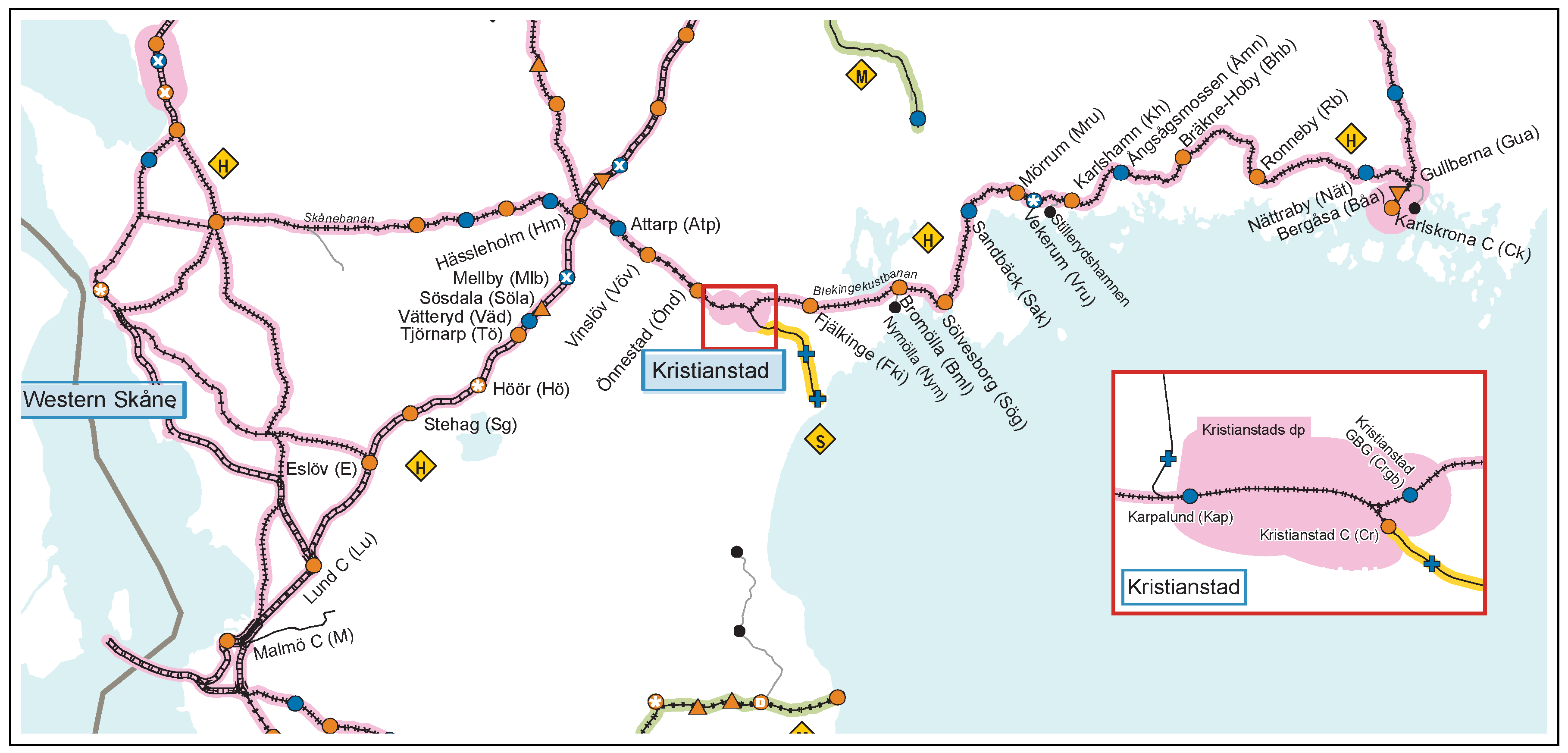
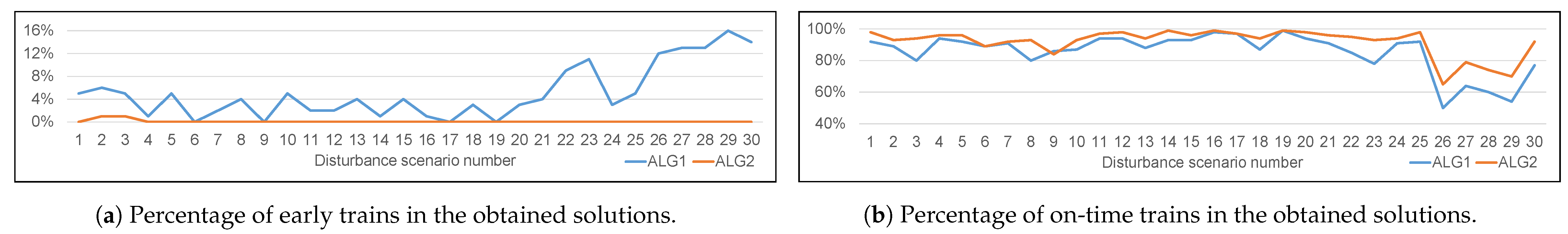
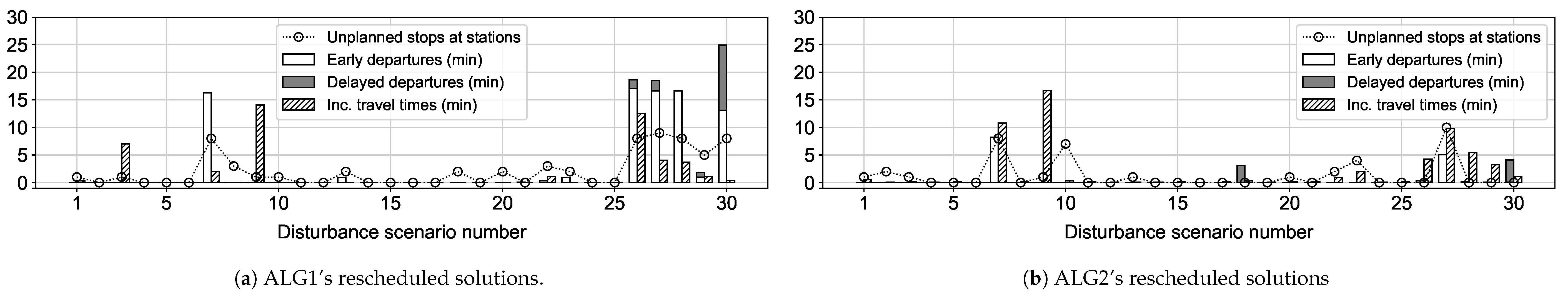
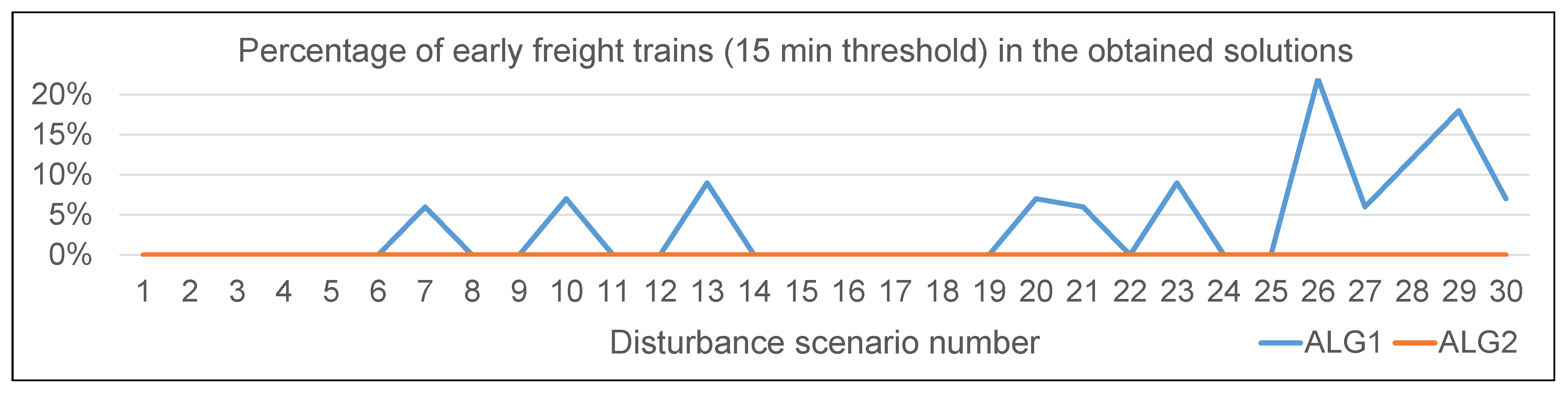
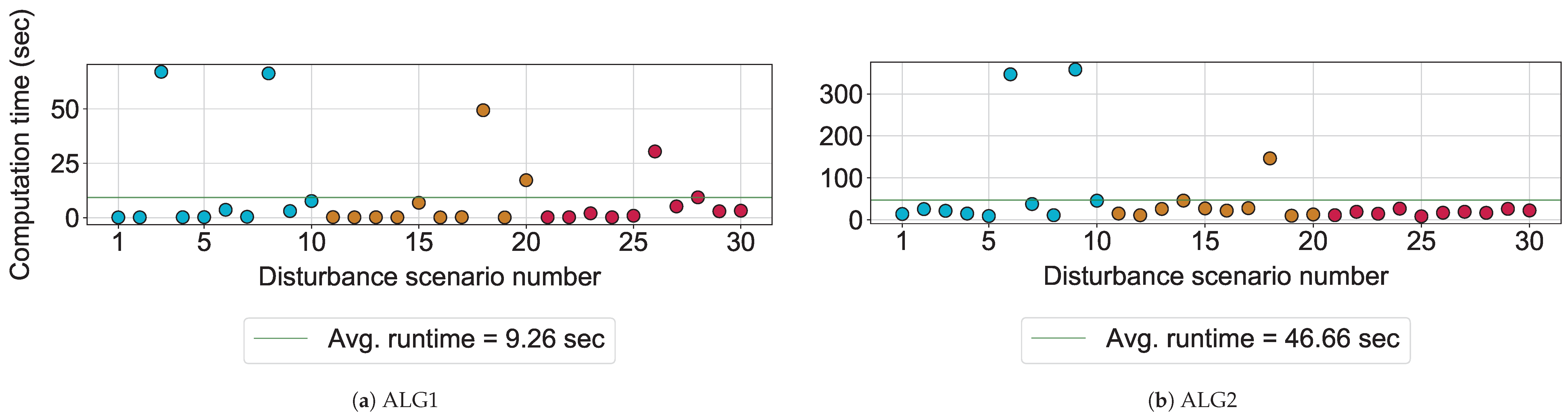
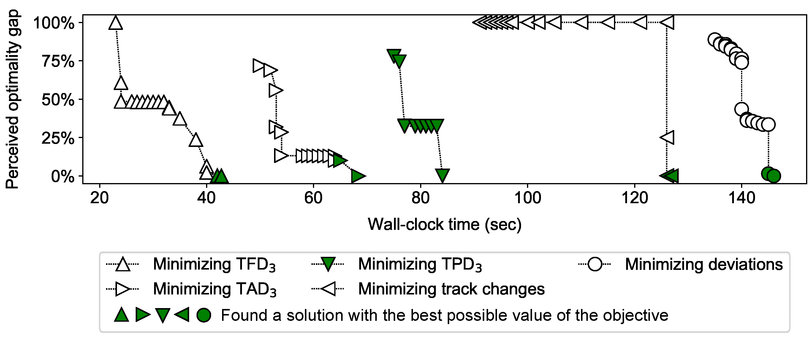


