On the Solutions of Second-Order Differential Equations with Polynomial Coefficients: Theory, Algorithm, Application

Abstract

The analysis of many physical phenomena is reduced to the study of linear differential equations with polynomial coefficients. The present work establishes the necessary and sufficient conditions for the existence of polynomial solutions to linear differential equations with polynomial coefficients of degree n, $n-1$, and $n-2$ respectively. We show that for $n\ge 3$ the necessary condition is not enough to ensure the existence of the polynomial solutions. Applying Scheffé’s criteria to this differential equation we have extracted n generic equations that are analytically solvable by two-term recurrence formulas. We give the closed-form solutions of these generic equations in terms of the generalized hypergeometric functions. For arbitrary n, three elementary theorems and one algorithm were developed to construct the polynomial solutions explicitly along with the necessary and sufficient conditions. We demonstrate the validity of the algorithm by constructing the polynomial solutions for the case of $n=4$. We also demonstrate the simplicity and applicability of our constructive approach through applications to several important equations in theoretical physics such as Heun and Dirac equations.

1. Introduction

Differential equations with polynomial coefficients have played an important role not only in understanding engineering and physics problems [1,2,3,4,5,6,7,8,9,10,11,12,13,14,15,16,17,18,19,20,21,22,23,24,25,26,27,28,29,30,31,32], but also as a source of inspiration for some of the most crucial results in special functions and orthogonal polynomials [33,34,35,36,37,38,39,40,41,42,43,44,45,46,47,48]. The classical differential equation

$$\left({\alpha }_2{r}^2+{\alpha }_{1}r+{\alpha }_0\right)y^{″}\left(r\right)+\left({\beta }_{1}r+{\beta }_0\right)y^{\prime }\left(r\right)-{\tau }_{0}y\left(r\right)=0,$$

(1)

has been a cornerstone of many fundamental results in special functions since the early work of L. Euler [33], see also References [47,48,49]. More recently, the Heun-type equation [41,42,43],

$$r\left({\alpha }_3{r}^2+{\alpha }_{2}r+{\alpha }_1\right)y^{″}\left(r\right)+\left({\beta }_2{r}^2+{\beta }_{1}r+{\beta }_0\right)y^{\prime }\left(r\right)-\left({\tau }_{1}r+{\tau }_0\right)y\left(r\right)=0,$$

(2)

has become a classic equation in mathematical physics. These two equations are members of the general differential equation

$$\begin{array}{cc}\hfill & P_n\left(r\right)y^{″}\left(r\right)+Q_{n-1}\left(r\right)y^{\prime }\left(r\right)-R_{n-2}\left(r\right)y\left(r\right)=0,n\ge 2,\hfill \\ \hfill & P_n\left(r\right)=\sum _{k=0}^n{\alpha }_k{r}^k,Q_{n-1}\left(r\right)=\sum _{k=0}^{n-1}{\beta }_k{r}^k,R_{n-2}\left(r\right)=\sum _{k=0}^{n-2}{\tau }_k{r}^k,\hfill \end{array}$$

(3)

where ${\left\{{\alpha }_k\right\}}_{k=0}^n$, ${\left\{{\beta }_k\right\}}_{k=0}^{n-1}$, ${\left\{{\tau }_k\right\}}_{k=0}^{n-2}$ are real parameters. We assume that the leading term of $R_{n-2}\ne 0$ and at least one of the leading terms ${\alpha }_n$ and ${\beta }_{n-1}$ is not zero. The purpose of the present work is to provide an answer to the following question:

“Under what conditions on the equation parameters ${\left\{{\alpha }_k\right\}}_{k=0}^n$, ${\left\{{\beta }_k\right\}}_{k=0}^{n-1}$, and ${\left\{{\tau }_k\right\}}_{k=0}^{n-2}$ does the differential Equation (3) have polynomial solutions? If it does have polynomial solutions, how can we construct them?”

With the general theory of linear differential equations as a guide [50,51], the zeros of the leading polynomial $P_n\left(r\right)$ classify the solutions of the Equation (3). The point $r=\zeta$ is called an ordinary point if $Q_{n-1}\left(r\right)/P_n\left(r\right)$ and $R_{n-2}\left(r\right)/P_n\left(r\right)$ are analytic functions at $r=\zeta$, or a regular singular point if $Q_{n-1}\left(r\right)/P_n\left(r\right)$ and $R_{n-2}\left(r\right)/P_n\left(r\right)$ are not analytic at $r=\zeta$ but the products $(r-\zeta )Q_{n-1}\left(r\right)/P_n\left(r\right)$ and ${(r-\zeta )}^2{R}_{n-2}\left(r\right)/P_n\left(r\right)$ are analytic at that point. Using this characterization of singularities, S. Bochner [48] classified the polynomial solutions of (1) in terms of the classical orthogonal polynomials. A different approach which depends on the parameters of the leading coefficient $P_n\left(r\right)$, was introduced in Reference [13] to study the polynomial solutions of (1). It was shown that there are seven possible nonzero leading polynomials depending on the combination of the nonzero ${\alpha }_i$ parameters, for $i=0,1,2$. By analyzing each of these cases, the authors [13] were able to explicitly construct all the polynomial solutions of Equation (1) in terms of hypergeometric functions along with the associated weight functions.

The nth-degree leading polynomial coefficient $P_n\left(r\right)$ of the differential Equation (3) contains $(2^{n+1}-1)$ nonzero polynomials that depend on the nonzero values of ${\alpha }_i$, $i=0,1,\dots ,n$. Out of this polynomial set, there are $2^n$ differential equations for which $r=0$ is an ordinary point, $(2^{n-1}+2^{n-2})$ differential equations for which $r=0$ is a regular singular point, and the remaining $(2^{n-2}-1)$ differential equations with irregular singular points that fall outside of the scope of this present work.

The criteria for polynomial solutions of second-order linear differential Equation (3) was introduced, using the Asymptotic Iteration Method, in References [52,53]:

Theorem 1.

[52,53] Given ${\lambda }_0\equiv {\lambda }_0\left(x\right)$ and $s_0\equiv s_0\left(x\right)$ in $C^{\infty }$, the differential equation $y^{″}={\lambda }_0\left(x\right)y^{\prime }+s_0\left(x\right)y$ has the general solution

$$y=exp\left(-\stackrel{x}{\int }\alpha \left(t\right)dt\right)\left[C_2+C_1\stackrel{x}{\int }exp\left(\stackrel{t}{\int }\left({\lambda }_0\left(\tau \right)+2\alpha \left(\tau \right)\right)d\tau \right)dt\right],$$

(4)

if, for some positive integer $m>0$,

$$\frac{s_m}{{\lambda }_m}=\frac{s_{m-1}}{{\lambda }_{m-1}}=\alpha \left(x\right),\mathrm{or}{\delta }_m\left(x\right)={\lambda }_m{s}_{m-1}-{\lambda }_{m-1}{s}_m=0,$$

(5)

where ${\lambda }_m={\lambda }_{m-1}^{\prime }+s_{m-1}+{\lambda }_0{\lambda }_m,$ and $s_m=s_{m-1}^{\prime }+s_0{\lambda }_m$. Further, the differential equation has a polynomial solution of degree m, if

$${\delta }_m\left(x\right)={\lambda }_m{s}_{m-1}-{\lambda }_{m-1}{s}_m=0.$$

(6)

With ${\lambda }_0\left(r\right)=-Q_{n-1}\left(r\right)/P_n\left(r\right)$ and $s_0\left(r\right)=R_{n-2}\left(r\right)/P_n\left(r\right)$, a simple algorithm based on Theorem 1 can be used to examine the polynomial solutions of (3).

The present work establishes polynomial solutions in simple and constructive forms to (3) along with all necessary and sufficient conditions they require. This work is done independently from that of Theorem 1, although can be verified using the Asymptotic Iteration Method.

The paper is organized as follows:

• In Section 2, we introduce the concept of a necessary but not sufficient condition to find polynomial solutions, and then demonstrate how the inverse square-root potential [22,23,24,25] is one such example that does not have polynomial solutions yet satisfies the necessary condition.
• In Section 3, Scheffé criteria is revised to analyze Equation (3) and to generate exactly solvable equations where the coefficients of their power series solutions are easily computed using a two-term recurrence relation. The closed form solutions of these equations are written in terms of the generalized hypergeometric functions

  $$\begin{array}{c}\hfill {}_p{F}_q\left(\begin{array}{ccc}{\alpha }_1,& \cdots ,& {\alpha }_p\\ {\beta }_1& \cdots ,& {\beta }_q\end{array};r\right)=\sum _{k=0}^{\infty }{\displaystyle \frac{{\prod }_{j=1}^p{\left({\alpha }_p\right)}_k}{{\prod }_{j=1}^q{\left({\alpha }_q\right)}_k}}{\displaystyle \frac{r^k}{k!}},\end{array}$$

  where the Pochhammer symbol ${\left(\alpha \right)}_k$ is defined in terms of the Gamma function as ${\left(\alpha \right)}_k=\alpha (\alpha +1)\cdots (\alpha +k-1)=\Gamma (\alpha +k)/\Gamma \left(\alpha \right)$.
• In Section 4 we present three theorems corresponding to the cases: (1) ${\alpha }_0\ne 0$, (2) ${\alpha }_0=0$, ${\alpha }_1\ne 0$, and (3) ${\alpha }_0={\alpha }_1={\beta }_0=0$, ${\alpha }_2\ne 0$ which are required to establish the polynomial solutions of Equation (3). We shall show that for the mth-degree polynomial solutions, there are $n+m-1$ conditions that ultimately assemble these polynomials. At the end of the section we briefly discuss the Mathematica^® program used to generate the solutions of these equations.
• Lastly, Section 5 demonstrates the validity of these constructions through the application of our results to some problems that have appeared in mathematics and physics literature.

2. A Necessary but Not Sufficient Condition

We begin by stating the necessary condition for the existence of polynomial solutions to the general differential equation given by (3):

Theorem 2.

A necessary condition for the differential Equation (3) to have a polynomial solution of degree m is

$${\tau }_{n-2}={\alpha }_{n}m(m-1)+{\beta }_{n-1}m,n=2,3,\dots .$$

(7)

Proof. 

Substitute the polynomial solution $y={\sum }_{i=0}^m{\mathcal{C}}_i{r}^i$ into the differential Equation (3). After collecting the common terms of the common r power, the necessary condition for the leading coefficient ${\mathcal{C}}_m$ to be nonzero is ${\tau }_{n-2}={\alpha }_{n}m(m-1)+{\beta }_{n-1}m$ for all $m\ge 0$ follows. □

For $n=2$, Equation (7) represents both the necessary and sufficient conditions for the polynomial solutions of (3). Although the condition (7) is necessary, it is not sufficient for $n\ge 3$ to guarantee the polynomial solutions of (3). There are precisely $n-2$ additional conditions that are sufficient to ensure the existence of such polynomials. These additional conditions can be understood as constraints that relate the remaining parameters of $R_{n-2}\left(r\right)$ with the coefficients ${\left\{{\alpha }_k\right\}}_{k=0}^n$ and ${\left\{{\beta }_k\right\}}_{k=0}^{n-1}$ in $P_n\left(r\right)$ and $Q_{n-1}\left(r\right)$, respectively. In later sections, we shall devise a procedure to find these sufficient conditions and provide a method of evaluating the corresponding polynomial solutions explicitly.

The remainder of the section investigates the inverse square-root potential. We shall show that despite satisfying the necessary condition in Theorem 2 that the Schrödinger equation with this potential as mentioned in the literature has no polynomial solutions, thus demonstrating that the condition (7) is necessary but not sufficient.

The Inverse Square-Root Potential

The exact solutions of the radial Schrödinger equation

$$-{\displaystyle \frac{d^2\psi \left(r\right)}{d{r}^2}}+\left(-\frac{v}{\sqrt{r}}+{\displaystyle \frac{l(l+1)}{r^2}}\right)\psi \left(r\right)=E\psi \left(r\right),v>0,r>0,\psi \left(0\right)=\psi (\infty )=0,$$

(8)

were recently studied by a number of authors [21,22,23,24,25]. The differential Equation (8) has two singular points, one regular at $r=0$ and another irregular at $r=\infty$ of rank 3 [50]. To analyze these singular points further, we employ a change of variables $z=\sqrt{2\kappa r}$, for some constant $\kappa$ to be determined shortly. Equation (8) may then be expressed as

$$z^2{\psi }^{″}\left(z\right)-z{\psi }^{\prime }\left(z\right)+\left(\left(\frac{\sqrt{2}v}{{\kappa }^{3/2}}+\frac{E}{{\kappa }^2}z\right)z^3-4l(l+1)\right)\psi \left(z\right)=0,\psi \left(0\right)=\psi (\infty )=0.$$

(9)

As $z\to 0$, the solution to the differential Equation (9) behaves asymptotically as the solution of the Euler equation, $z^2{\psi }^{″}\left(z\right)-z{\psi }^{\prime }\left(z\right)-4l(l+1)\psi \left(z\right)=0$, which has a physically acceptable solution $\psi \left(z\right)\sim z^{2(l+1)}$. Meanwhile as $z\to \infty$, the solution to the differential equation behaves asymptotically as the solution of

$${\psi }^{″}\left(z\right)+\left(\frac{\sqrt{2}v}{{\kappa }^{3/2}}-z\right)z\psi \left(z\right)=0.$$

To examine the solution of this equation we complete the square to

$$-{\psi }^{″}\left(z\right)+{\left(\frac{v}{\sqrt{2{\kappa }^3}}-z\right)}^2\psi \left(z\right)={\left(\frac{v}{\sqrt{2{\kappa }^3}}\right)}^2\psi \left(z\right).$$

(10)

The substitution $x=((v/\sqrt{2{\kappa }^3})-z)$ allows us to compare the solution of the equation to the solvable Schröinger equation with the harmonic oscillator potential, as $z\to \infty$, via

$$\psi \left(z\right)=exp\left(-{\int }^z(u+\lambda )du\right)=exp\left(-\left(\frac{z^2}{2}+\lambda z\right)\right),\lambda =-\frac{v}{\sqrt{2{\kappa }^3}}.$$

(11)

Hence, we may assume the solution of Equation (9) to be

$$\psi \left(z\right)=N{z}^{2(l+1)}exp\left(-\left({\displaystyle \frac{z^2}{2}}+\lambda z\right)\right)f\left(z\right),\lambda =-\frac{v}{\sqrt{2{\kappa }^3}}<0,$$

(12)

up to a normalization constant N. Upon substituting the ansatz solution (12) into Equation (9), we obtain a second-order differential equation (an example of a biconfluent Heun equation [41]) for $f\left(z\right)$ as

$$z{f}^{″}\left(z\right)-\left[2z^2+2\lambda z-3-4l\right]f^{\prime }\left(z\right)+\left[\left({\lambda }^2-4(l+1)\right)z-(3+4l)\lambda \right]f\left(z\right)=0,$$

(13)

subject to $\kappa =\sqrt{-E}$. Clearly, Equation (13) is of the form of Equation (3) with $n=3$ with the parameters ${\alpha }_3={\alpha }_2=0$, ${\alpha }_1=1$, ${\beta }_2=-2$, ${\beta }_1=-2\lambda$, ${\beta }_0=3+4l$, ${\tau }_1=-{\lambda }^2+4(l+1)$, and ${\tau }_0=(3+4l)\lambda$. Using Theorem 2, for the existence of an mth-degree polynomial solution it is necessary that

$${\lambda }^2-4(l+1)=2m,m=0,1,2,\dots .$$

(14)

Note that this result can be also deduced using the Bethe Ansatz method [12,54]. On the other hand, an application of the Frobenius method establishes the following three-term recurrence relation for the coefficients of the polynomial solutions $f_m\left(r\right)={\sum }_{j=0}^m{\mathcal{C}}_j{r}^j$:

$$(j+1)\left(j+3+4l\right){\mathcal{C}}_{j+1}-\lambda \left(2j+3+4l\right){\mathcal{C}}_j-\left(2j-{\lambda }^2+4l+2\right){\mathcal{C}}_{j-1}=0,$$

(15)

where $j=0,1,2,\dots ,m,m+1$ and $C_j=0$ for $j<0$. Implementing the necessary condition (14), with $\lambda =-\sqrt{4+4l+2m}<0$, Equation (15) then reads

$$(j+1)\left(j+3+4l\right){\mathcal{C}}_{j+1}+\sqrt{4+4l+2m}\left(2j+3+4l\right){\mathcal{C}}_j+2\left(m-j+1\right){\mathcal{C}}_{j-1}=0.$$

(16)

The consistency of the linear homogeneous system generated by the three-term recurrence relation (16), for $j=0,1,\cdots ,m+1$, enforces the vanishing of the determinant, denoted by ${\mathsf{\Delta }}_{(m+1)}$, that establish the sufficient condition

$${\mathsf{\Delta }}_{m+1}=\left|\begin{array}{ccccccc}{S}_0& T_1& & & & & \\ {\gamma }_1& S_1& T_2& & & & \\ & {\gamma }_2& S_2& T_3& & & \\ & & \ddots & \ddots & \ddots & & \\ & & & {\gamma }_{m-2}& S_{m-2}& T_{m-1}& \\ & & & & {\gamma }_{m-1}& S_{m-1}& T_m\\ & & & & & {\gamma }_m& S_m\end{array}\right|,\begin{array}{c}\hfill \mathrm{where}\\ \hfill S_j& =(2j+3+4l)\sqrt{4+4l+2m},\hfill \\ \hfill T_j& =j(j+2+4l),\hfill \\ \hfill {\gamma }_j& =2(m-j+1).\hfill \end{array}$$

(17)

Therefore, if the determinant ${\mathsf{\Delta }}_{m+1}$ is different than zero, the only possible solution to the linear system is the trivial solution (i.e., the zero solution). Hence any nonzero value of the determinant ${\mathsf{\Delta }}_{m+1}$ is an indication that a polynomial solution is not possible, which is the case for the coefficients of Equation (13).

Remark 1.

The point here is not solving the Schrödinger equation with the inverse-root potential; this is already done in several manuscripts [21,22,23,24,25]. We stress that the necessary condition is not enough to guarantee polynomial solutions. Also, the necessary and sufficient constraints must have common roots that are physically acceptable.

Remark 2.

In Reference [55], the author claims the existence of polynomial solutions of a differential equation which matches (13) that satisfy the necessary condition (7). The author missed the possibility of the non-vanishing determinant (4), in his work, for some ${\beta }_0$ and ${\beta }_2$.

Remark 3.

For the applications in physics, there is nothing special about the necessity of the polynomial solutions. However, the problem of the existence of polynomial solutions is important. Studying the problem in its general form and developing mathematical tools to treat it is significant on its own.

3. Scheffé’s Criteria: Two-Term Recurrence Relation

Generally speaking, recurrence relations with more than two terms are difficult to solve explicitly. Differential equations that are known to have a two-term recurrence relation for their power series solutions guarantee the solvability of such equations.

In a paper presented to the American Mathematical Society (1941), H. Scheffé [34] establishes criteria for the necessary and sufficient conditions for differential equations of the form

$$p_2\left(r\right)u^{″}\left(r\right)+p_1\left(r\right)u^{\prime }\left(r\right)+p_0\left(r\right)u\left(r\right)=0,$$

(18)

to have a two-term recurrence relation. Here $p_j\left(r\right)\ne 0$, $j=0,1,2,$ are analytic functions (not necessarily polynomials) in some region consisting of all points in an arbitrary neighbourhood of a regular singular point $r=r_0$ except the point $r_0$ itself. We adopt this criterion to examine the differential Equation (18) with

$$p_2\left(r\right)=\sum _{k=0}^n{\alpha }_k{r}^k,p_1\left(r\right)=\sum _{k=0}^{n-1}{\beta }_k{r}^k,p_0\left(r\right)=\sum _{k=0}^{n-2}{\gamma }_k{r}^k,n\ge 2,$$

(19)

and provide a formula for the two-term recurrence relation. Without loss of generality, we shall take the ordinary or singular point as $r=0$, otherwise a simple shifting of r is applied first.

Theorem 3.

The necessary and sufficient conditions for the differential Equation (18) to have a two-term recurrence relation between successive coefficients in its series solution, relative to the ordinary or regular singular point $r=0$, is that in the neighbourhood of $r=0$ Equation (18) can be written as:

$$\begin{array}{cc}\hfill [q_{2,0}+q_{2,h}{r}^h]& r^{2-m}{u}^{″}\left(r\right)+[q_{1,0}+q_{1,h}{r}^h]r^{1-m}{u}^{\prime }\left(r\right)+[q_{0,0}+q_{0,h}{r}^h]r^{-m}u\left(r\right)=0,\hfill \end{array}$$

(20)

where, for $m\in \mathbb{Z}$, $h\in {\mathbb{Z}}^{+}$,

$$q_j\left(r\right)\equiv \sum _{k=0}^{\infty }{q}_{j,k}{r}^k=p_j\left(r\right)r^{m-j},j=0,1,2,$$

(21)

and at least one of the product $q_{j,0}{q}_{i,h}$, for $i,j=0,1,2$, is nonzero. The two-term recurrence formula is given by

$$\begin{array}{c}\hfill c_k=-{\displaystyle \frac{q_{2,h}(k+\lambda -h)(k+\lambda -h-1)+q_{1,h}(k+\lambda -h)+q_{0,h}}{q_{2,0}(k+\lambda )(k+\lambda -1)+q_{1,0}(k+\lambda )+q_{0,0}}}{c}_{k-h},c_0\ne 0,\end{array}$$

(22)

where $\lambda ={\lambda }_1,{\lambda }_2$ are the roots of the indicial equation

$$q_{2,0}\lambda (\lambda -1)+q_{1,0}\lambda +q_{0,0}=0.$$

(23)

The closed form of the series solution can be written in terms of the generalized hypergeometric function as

$$\begin{array}{cc}\hfill u& (r;\lambda )=r^{\lambda }\sum _{k=0}^{\infty }{c}_{hk}{r}^{hk}\hfill \\ \hfill & =r^{\lambda }{}_3{F}_2\left(1,\frac{2\lambda -1}{2h}+\frac{q_{1,h}}{2h{q}_{2,h}}-\frac{\sqrt{{(q_{1,h}-q_{2,h})}^2-4q_{0,h}{q}_{2,h}}}{2h{q}_{2,h}},\right.\frac{2\lambda -1}{2h}+\frac{q_{1,h}}{2h{q}_{2,h}}+\frac{\sqrt{{(q_{1,h}-q_{2,h})}^2-4q_{0,h}{q}_{2,h}}}{2h{q}_{2,h}};\hfill \\ \hfill & 1+\frac{2\lambda -1}{2h}+\frac{q_{1,0}}{2h{q}_{2,0}}-\frac{\sqrt{{(q_{1,0}-q_{2,h})}^2-4q_{0,0}{q}_{2,0}}}{2h{q}_{2,0}},\left.1+\frac{2\lambda -1}{2h}+\frac{q_{1,0}}{2h{q}_{2,0}}+\frac{\sqrt{{(q_{1,0}-q_{2,h})}^2-4q_{0,0}{q}_{2,0}}}{2h{q}_{2,0}};-\frac{q_{2,h}}{q_{2,0}}{r}^h\right).\hfill \end{array}$$

(24)

As an example, we consider the differential equation

$$\begin{array}{c}\hfill ({\alpha }_2{r}^2+{\alpha }_{1}r+{\alpha }_0)u^{″}\left(r\right)+({\beta }_{1}r+{\beta }_0)u^{\prime }\left(r\right)+{\gamma }_{0}u\left(r\right)=0,\end{array}$$

(25)

mentioned in the introduction. We want to extract the possible equations that have two-term recurrence relations between successive coefficients in their series solutions.

Comparing Equation (25) with (20), we find that $h+2-m=2$ and $h+2-m=2>2-m\ge 0$, which leads to $h=m$, $2>2-m\ge 0$. Consequently $0<m\le 2$ which gives us two cases: $(m,h)=(1,1)$, and $(m,h)=(2,2)$.

• In the case of $m=1$ and $h=1$, Equation (20) reads:

  $$[q_{2,0}+q_{2,1}r]r{u}^{″}\left(r\right)+[q_{1,0}+q_{1,1}r]u^{\prime }\left(r\right)+[q_{0,0}+q_{0,1}r]r^{-1}u\left(r\right)=0,$$

  (26)

  and the corresponding Equation (25) with $q_{2,0}={\alpha }_1$, $q_{2,h=1}={\alpha }_2$, $q_{1,0}={\beta }_0$, $q_{1,h=1}={\beta }_1$, $q_{0,h=1}={\gamma }_0$ and $q_{0,0}=0$ reads

  $$({\alpha }_{1}r+{\alpha }_2{r}^2)u^{″}\left(r\right)+({\beta }_0+{\beta }_{1}r)u^{\prime }\left(r\right)+{\gamma }_{0}u\left(r\right)=0.$$

  (27)
  The two-term recurrence formula for the solution of Equation (27) is

  $$c_k=-{\displaystyle \frac{{\alpha }_2(k+\lambda -1)(k+\lambda -2)+{\beta }_1(k+\lambda -1)+{\gamma }_0}{{\alpha }_1(k+\lambda )(k+\lambda -1)+{\beta }_0(k+\lambda )}}{c}_{k-1},c_0=1,$$

  (28)

  where $\lambda$ are the zeros of the indicial equation ${\alpha }_1\lambda (\lambda -1)+{\beta }_0\lambda =0$, namely, $\lambda =0$, and $\lambda =1-{\beta }_0/{\alpha }_1$.
  The closed form solutions in terms of the Gauss hypergeometric functions, respectively, are:

  $$\begin{array}{cc}\hfill & u_1(r,\lambda =0)\hfill \\ \hfill & ={}_2{F}_1\left(-\frac{1}{2}+\frac{{\beta }_1}{2{\alpha }_2}-\frac{\sqrt{{({\alpha }_2-{\beta }_1)}^2-4{\alpha }_2{\gamma }_0}}{2{\alpha }_2},-\frac{1}{2}+\frac{{\beta }_1}{2{\alpha }_2}+\frac{\sqrt{{({\alpha }_2-{\beta }_1)}^2-4{\alpha }_2{\gamma }_0}}{2{\alpha }_2};\frac{{\beta }_0}{{\alpha }_1};-\frac{{\alpha }_2}{{\alpha }_1}r\right),\hfill \end{array}$$

  (29)

  and

  $$\begin{array}{cc}\hfill & u_2(r,\lambda =1-\frac{{\beta }_0}{{\alpha }_1})=r^{1-\frac{{\beta }_0}{{\alpha }_1}}\hfill \\ \hfill & \times {}_2{F}_1\left(\frac{1}{2}+\frac{{\beta }_1}{2{\alpha }_2}-\frac{{\beta }_0}{{\alpha }_1}+\frac{\sqrt{{({\alpha }_2-{\beta }_1)}^2-4{\alpha }_2{\gamma }_0}}{2{\alpha }_1{\alpha }_2},\frac{1}{2}+\frac{{\beta }_1}{2{\alpha }_2}+\frac{{\beta }_0}{{\alpha }_1}+\frac{\sqrt{{({\alpha }_2-{\beta }_1)}^2-4{\alpha }_2{\gamma }_0}}{2{\alpha }_1{\alpha }_2};2-\frac{{\beta }_0}{{\alpha }_1};-\frac{{\alpha }_2}{{\alpha }_1}r\right).\hfill \end{array}$$

  (30)
• In this case of $m=2$ and $h=2$, Equation (20) reads

  $$[q_{2,0}+q_{2,h}{r}^2]u^{″}\left(r\right)+[q_{1,0}+q_{1,h}{r}^2]r^{-1}{u}^{\prime }\left(r\right)+[q_{0,0}+q_{0,h}{r}^2]r^{-2}u\left(r\right)=0,$$

  (31)

  and the corresponding Equation (25) reads

  $$({\alpha }_0+{\alpha }_2{r}^2)u^{″}\left(r\right)+{\beta }_{1}r{u}^{\prime }\left(r\right)+{\gamma }_{0}u\left(r\right)=0.$$

  (32)
  The two-term recurrence relation for the solutions of Equation (32) reads

  $$\begin{array}{c}\hfill c_k=-{\displaystyle \frac{{\alpha }_2(k+\lambda -2)(k+\lambda -3)+{\beta }_1(k+\lambda -2)+{\gamma }_0}{{\alpha }_0(k+\lambda )(k+\lambda -1)}}{c}_{k-2},k\ge 2,\end{array}$$

  (33)

  where, $\lambda$ are the roots of the indicial equation $\lambda (\lambda -1)=0$, ${\alpha }_0\ne 0$, with closed form solutions

  $$\begin{array}{cc}\hfill & u_1(r,\lambda =0)\hfill \\ \hfill & ={}_2{F}_1\left(\frac{{\beta }_1}{4{\alpha }_2}-\frac{1}{4}-\frac{\sqrt{{({\alpha }_2-{\beta }_1)}^2-4{\alpha }_2{\gamma }_0}}{4{\alpha }_2},\frac{{\beta }_1}{4{\alpha }_2}-\frac{1}{4}+\frac{\sqrt{{({\alpha }_2-{\beta }_1)}^2-4{\alpha }_2{\gamma }_0}}{4{\alpha }_2};\frac{1}{2};-\frac{{\alpha }_2}{{\alpha }_0}{r}^2\right),\hfill \end{array}$$

  (34)

  and

  $$\begin{array}{cc}\hfill & u_2(r,\lambda =1)\hfill \\ \hfill & =r{}_2{F}_1\left(\frac{{\beta }_1}{4{\alpha }_2}+\frac{1}{4}-\frac{\sqrt{{({\alpha }_2-{\beta }_1)}^2-4{\alpha }_2{\gamma }_0}}{4{\alpha }_2},\frac{{\beta }_1}{4{\alpha }_2}+\frac{1}{4}+\frac{\sqrt{{({\alpha }_2-{\beta }_1)}^2-4{\alpha }_2{\gamma }_0}}{4{\alpha }_2};\frac{3}{2};-\frac{{\alpha }_2}{{\alpha }_0}{r}^2\right).\hfill \end{array}$$

  (35)

Remark 4.

For the admissible values of the equation parameters, the recurrence relations (28) and (33) are generic formulas for the two-term recurrence relations for the series solutions of the differential Equations (27) and (32) respectively. That is to say, by assigning admissible values of the parameters, (27) and (32) will generate solvable differential equations.

Remark 5.

Polynomial solutions for the differential Equations (27) and (32) can be easily obtained using suitable values of the equation parameters to terminate the recurrence relations (28) and (33).

As a second example we consider the differential equation

$$\left({\alpha }_3{r}^3+{\alpha }_2{r}^2+{\alpha }_{1}r+{\alpha }_0\right)y^{″}\left(r\right)+\left({\beta }_2{r}^2+{\beta }_{1}r+{\beta }_0\right)y^{\prime }\left(r\right)+\left({\gamma }_{1}r+{\gamma }_0\right)y\left(r\right)=0.$$

(36)

As before, we want to extract the equations with a two-term recurrence relationship between successive coefficients in its series solution. We note by comparing Equation (36) and Equation (20) that $h+2-m=3$ and $3>2-m\ge 0$, so $-1<m\le 2$. Three cases $(m,h)=(0,1),(m,h)=(1,2)$ and $(m,h)=(2,3)$ follow from these constraints, and we consider each of these cases separately:

• In the case where $m=0$ and $h=1$, Equation (20) reads, with $q_{2,h=2}={\alpha }_3$, $q_{1,h=2}={\beta }_2$, $q_{0,h=2}={\gamma }_1$, $q_{2,0}={\alpha }_2$, $q_{1,0}={\beta }_1$, and $q_{0,0}={\gamma }_0$

  $$\begin{array}{c}\hfill [{\alpha }_2{r}^2+{\alpha }_3{r}^3]u^{″}\left(r\right)+[{\beta }_{1}r+{\beta }_2{r}^2]u^{\prime }\left(r\right)+({\gamma }_0+{\gamma }_{1}r)u\left(r\right)=0,{\gamma }_0\ne 0,\end{array}$$

  (37)
  For this differential equation, the recurrence relation (22) implies

  $$\begin{array}{c}\hfill c_k=-{\displaystyle \frac{{\alpha }_3(k+\lambda -1)(k+\lambda -2)+{\beta }_2(k+\lambda -1)+{\gamma }_1}{{\alpha }_2(k+\lambda )(k+\lambda -1)+{\beta }_1(k+\lambda )+{\gamma }_0}}{c}_{k-1},c_0\ne 0,\end{array}$$

  (38)

  where $\lambda$ are the roots of the indicial equation ${\alpha }_2\lambda (\lambda -1)+{\beta }_1\lambda +{\gamma }_0=0$. The values of $\lambda$ with (38) gives the following two linearly independent series solutions for the differential Equation (37):

  $$\begin{array}{cc}\hfill & u_1\left(r\right)=r^{\frac{{\alpha }_2-{\beta }_1+\sqrt{{({\alpha }_2-{\beta }_1)}^2-4{\alpha }_2{\gamma }_0}}{2{\alpha }_2}}\hfill \\ \hfill & \times {}_2{F}_1\left(\frac{{\beta }_2}{2{\alpha }_3}-\frac{{\beta }_1}{2{\alpha }_2}+\frac{\sqrt{{({\alpha }_2-{\beta }_1)}^2-4{\alpha }_2{\gamma }_0}}{2{\alpha }_2}-\frac{\sqrt{{({\alpha }_3-{\beta }_2)}^2-4{\alpha }_3{\gamma }_1}}{2{\alpha }_3},\right.\hfill \\ \hfill & \frac{{\beta }_2}{2{\alpha }_3}-\frac{{\beta }_1}{2{\alpha }_2}+\frac{\sqrt{{({\alpha }_2-{\beta }_1)}^2-4{\alpha }_2{\gamma }_0}}{2{\alpha }_2}+\frac{\sqrt{{({\alpha }_3-{\beta }_2)}^2-4{\alpha }_3{\gamma }_1}}{2{\alpha }_3};\left.\frac{{\alpha }_2+\sqrt{{({\alpha }_2-{\beta }_1)}^2-4{\alpha }_2{\gamma }_0}}{{\alpha }_2};-\frac{{\alpha }_3}{{\alpha }_2}r\right),\hfill \end{array}$$

  (39)

  and

  $$\begin{array}{cc}\hfill & u_2\left(r\right)=r^{\frac{{\alpha }_2-{\beta }_1-\sqrt{{({\alpha }_2-{\beta }_1)}^2-4{\alpha }_2{\gamma }_0}}{2{\alpha }_2}}\hfill \\ & \times {}_2{F}_1\left(\frac{{\beta }_2}{2{\alpha }_3}-\frac{{\beta }_1}{2{\alpha }_2}-\frac{\sqrt{{({\alpha }_2-{\beta }_1)}^2-4{\alpha }_2{\gamma }_0}}{2{\alpha }_2}-\frac{\sqrt{{({\alpha }_3-{\beta }_2)}^2-4{\alpha }_3{\gamma }_1}}{2{\alpha }_3},\right.\hfill \\ \hfill & \frac{{\beta }_2}{2{\alpha }_3}-\frac{{\beta }_1}{2{\alpha }_2}-\frac{\sqrt{{({\alpha }_2-{\beta }_1)}^2-4{\alpha }_2{\gamma }_0}}{2{\alpha }_2}+\frac{\sqrt{{({\alpha }_3-{\beta }_2)}^2-4{\alpha }_3{\gamma }_1}}{2{\alpha }_3};\left.\frac{{\alpha }_2-\sqrt{{({\alpha }_2-{\beta }_1)}^2-4{\alpha }_2{\gamma }_0}}{{\alpha }_2};-\frac{{\alpha }_3}{{\alpha }_2}r\right).\hfill \end{array}$$

  (40)
• In the case where $m=1$ and $h=2$, Equation (20) reads,

  $$[{\alpha }_{1}r+{\alpha }_3{r}^3]u^{″}\left(r\right)+[{\beta }_0+{\beta }_2{r}^2]u^{\prime }\left(r\right)+{\gamma }_{1}ru\left(r\right)=0,{\beta }_0\ne 0,$$

  (41)
  For this differential equation, the recurrence relation (22) implies

  $$\begin{array}{c}\hfill c_k=-{\displaystyle \frac{{\alpha }_3(k+\lambda -2)(k+\lambda -3)+{\beta }_2(k+\lambda -2)+{\gamma }_1}{{\alpha }_1(k+\lambda )(k+\lambda -1)+{\beta }_0(k+\lambda )}}{c}_{k-2},\end{array}$$

  (42)

  where $\lambda$ are the roots of the indicial equation $a_1\lambda (\lambda -1)+b_0\lambda =0$. The values of $\lambda$ with (42) gives the following two linearly independent series solutions for the differential Equation (41):

  $$\begin{array}{cc}\hfill u_1\left(r\right)& ={}_2{F}_1\left(\frac{{\beta }_2}{4{\alpha }_3}-\frac{1}{4}-\frac{\sqrt{{({\alpha }_3-{\beta }_2)}^2-4{\alpha }_3{\gamma }_1}}{4{\alpha }_3},\frac{{\beta }_2}{4{\alpha }_3}-\frac{1}{4}+\frac{\sqrt{{({\alpha }_3-{\beta }_2)}^2-4{\alpha }_3{\gamma }_1}}{4{\alpha }_3};\frac{{\alpha }_1+{\beta }_0}{2{\alpha }_1};-\frac{{\alpha }_3{r}^2}{{\alpha }_1}\right),\hfill \end{array}$$

  (43)

  and

  $$\begin{array}{cc}\hfill u& {}_2\left(r\right)=r^{1-\frac{{\beta }_0}{{\alpha }_1}}\times \hfill \end{array}$$

  (44)

  $$\begin{array}{cc}\hfill & {}_2{F}_1\left(\frac{1}{4}+\frac{{\beta }_2}{4{\alpha }_3}-\frac{{\beta }_0}{2{\alpha }_1}-\frac{\sqrt{{({\alpha }_3-{\beta }_2)}^2-4{\alpha }_3{\gamma }_1}}{4{\alpha }_3},\frac{1}{4}+\frac{{\beta }_2}{4{\alpha }_3}-\frac{{\beta }_0}{2{\alpha }_1}+\frac{\sqrt{{({\alpha }_3-{\beta }_2)}^2-4{\alpha }_3{\gamma }_1}}{4{\alpha }_3};\frac{3}{2}-\frac{{\beta }_0}{2{\alpha }_1};-\frac{{\alpha }_3{r}^2}{{\alpha }_1}\right).\hfill \end{array}$$

  (45)
• In the case where $m=2$ and $h=3$, Equation (20) reads,

  $$({\alpha }_0+{\alpha }_3{r}^3)u^{″}\left(r\right)+{\beta }_2{r}^2{u}^{\prime }\left(r\right)+{\gamma }_{1}ru\left(r\right)=0,{\alpha }_0\ne 0,$$

  (46)
  For this differential equation, the recurrence relation (22) implies

  $$\begin{array}{c}\hfill c_k=-{\displaystyle \frac{{\alpha }_3(k+\lambda -3)(k+\lambda -4)+{\beta }_2(k+\lambda -3)+{\gamma }_1}{{\alpha }_0(k+\lambda )(k+\lambda -1)}}{c}_{k-3},c_0\ne 0,\end{array}$$

  (47)

  where $\lambda$ are the roots of the indicial equation ${\alpha }_0\lambda (\lambda -1)=0$. The values of $\lambda$ with (47) gives the following two linearly independent series solutions for the differential Equation (46):

  $$\begin{array}{cc}\hfill u_1\left(r\right)& ={}_2{F}_1\left(-\frac{\sqrt{{({\alpha }_3-{\beta }_2)}^2-4{\alpha }_3{\gamma }_1}+{\alpha }_3-{\beta }_2}{6{\alpha }_3},\frac{\sqrt{{({\alpha }_3-{\beta }_2)}^2-4{\alpha }_3{\gamma }_1}-{\alpha }_3+{\beta }_2}{6{\alpha }_3};\frac{2}{3};-\frac{{\alpha }_3}{{\alpha }_0}{r}^3\right),\hfill \end{array}$$

  (48)

  and

  $$\begin{array}{c}\hfill u_2\left(r\right)=r{}_2{F}_1\left(\frac{-\sqrt{{({\alpha }_3-{\beta }_2)}^2-4{\alpha }_3{\gamma }_1}+{\alpha }_3+{\beta }_2}{6{\alpha }_3},\frac{\sqrt{{({\alpha }_3-{\beta }_2)}^2-4{\alpha }_3{\gamma }_1}+{\alpha }_3+{\beta }_2}{6{\alpha }_3};\frac{4}{3};-\frac{{\alpha }_3}{{\alpha }_0}{r}^3\right).\end{array}$$

  (49)

Remark 6.

When the coefficients of the differential Equation (18) are polynomials, there are n generic equations with series solutions explicitly found using the two-term recurrence relation (22). The closed-form solutions of these equations are given by (24). Indeed, for $h+2-m=n$, $n>2-m\ge 0$, we have n cases given $h=n+m-2$, $2-n<m\le 2$, $n\ge 2$. These n equations are as follows (See Theorem 3):

$$\begin{array}{c}\hfill \left\{\begin{array}{cc}({\alpha }_0+{\alpha }_n{r}^n)y^{″}+{\beta }_{n-1}{r}^{n-1}{y}^{\prime }+{\gamma }_{n-2}{r}^{n-2}y=0,\hfill & {\alpha }_0\ne 0\hfill \\ ({\alpha }_{1}r+{\alpha }_n{r}^n)y^{″}+({\beta }_0+{\beta }_{n-1}{r}^{n-1})y^{\prime }+{\gamma }_{n-2}{r}^{n-2}y=0,\hfill & {\beta }_0\ne 0\hfill \\ ({\alpha }_2{r}^2+{\alpha }_n{r}^n)y^{″}+({\beta }_{1}r+{\beta }_{n-1}{r}^{n-1})y^{\prime }+({\gamma }_0+{\gamma }_{n-2}{r}^{n-2})y=0,\hfill & {\gamma }_0\ne 0\hfill \\ ({\alpha }_3{r}^3+{\alpha }_n{r}^n)y^{″}+({\beta }_2{r}^2+{\beta }_{n-1}{r}^{n-1})y^{\prime }+({\gamma }_{1}r+{\gamma }_{n-2}{r}^{n-2})y=0,\hfill \\ ({\alpha }_4{r}^4+{\alpha }_n{r}^n)y^{″}+({\beta }_3{r}^3+{\beta }_{n-1}{r}^{n-1})y^{\prime }+({\gamma }_2{r}^2+{\gamma }_{n-2}{r}^{n-2})y=0,\hfill \\ ⋮\hfill \\ ({\alpha }_{n-1}{r}^{n-1}+{\alpha }_n{r}^n)y^{″}+({\beta }_{n-2}{r}^{n-2}+{\beta }_{n-1}{r}^{n-1})y^{\prime }+({\gamma }_{n-3}{r}^{n-3}+{\gamma }_{n-2}{r}^{n-2})y=0.\hfill \end{array}\right.\end{array}$$

(50)

4. Theorems and Algorithm

In this section we present three elementary theorems that classify the polynomial solutions of the general differential Equation (3). Following that, we will give a brief description of the Mathematica^® program that was developed to accompany the present work. A link to the complete program, available for direct use, is also provided for direct applications of these theorems.

4.1. Theorems

Theorem 4 applies to $2^n$ equations of (3) and gives a recurrence relation needed to compute polynomial solutions in the neighbourhood of an ordinary point. Theorems 5 and 6 give the polynomial solutions for the $2^{n-1}+2^{n-2}$ equations from (3) about a regular singular point. The proofs of Theorems 4 and 5 may be found in the Appendix A, while the proof of Theorem 6 follows closely to the proof of Theorem 5 and is therefore omitted.

Theorem 4.

$({\alpha }_{\mathbf{0}}\ne \mathbf{0})$

For ${\alpha }_0\ne 0$, the second-order linear differential Equation (3) admits the solution $y\left(r\right)={\mathcal{P}}_m\left(r\right)={\sum }_{i=0}^m{\mathcal{C}}_i{r}^i$ in the neighbourhood of the ordinary point $r=0$ and valid to the nearest nonzero singular point of ${\mathcal{P}}_m\left(r\right)=0$. Here ${\mathcal{P}}_m\left(r\right)$ is an mth-degree polynomial if

$$\sum _{j=0}^n\left[{\alpha }_{n-j}(\ell -n+j+2)(\ell -n+j+1)+{\beta }_{n-j-1}(\ell -n+j+2)-{\tau }_{n-j-2}\right]{\mathcal{C}}_{\ell -n+j+2}=0,$$

(51)

for all $\ell =0,1,2,\dots ,m+n-2$, and ${\tau }_i={\beta }_i=0$ if $i<0$. The equation corresponding to the value of $\ell =m+n-2$ gives the necessary condition (7) for the existence of the mth-degree polynomial solution

$${\tau }_{n-2}={\alpha }_{n}m(m-1)+{\beta }_{n-1}m,m=0,1,2,\dots .$$

(52)

The remaining $(m+n-2)$ linear equations consist of $(n-2)$ sufficient conditions that relate ${\left\{{\alpha }_k\right\}}_{k=0}^n$ and ${\left\{{\beta }_k\right\}}_{k=0}^{n-1}$ with ${\left\{{\tau }_k\right\}}_{k=0}^{n-2}$, in addition to the m linear equations required to evaluate the coefficients ${\left\{{\mathcal{C}}_i\right\}}_{i=1}^m$ of the polynomial solution in terms of ${\mathcal{C}}_0\ne 0$.

Theorem 5.

$({\alpha }_{\mathbf{0}}=\mathbf{0},{\alpha }_{\mathbf{1}}\ne \mathbf{0})$

For ${\alpha }_0=0$ and ${\alpha }_1\ne 0$, the second-order linear differential Equation (3) admits the solution $y\left(r\right)=r^s{\mathcal{P}}_m\left(r\right)=r^s{\sum }_{i=0}^m{\mathcal{C}}_i{r}^i$ in the neighbourhood of the regular singular point $r=0$, where ${\mathcal{P}}_m\left(r\right)$ is an mth-degree polynomial if

$$\sum _{j=0}^{n-1}\left[{\alpha }_{n-j}(\ell -n+j+s+2)(\ell -n+j+s+1)+{\beta }_{n-j-1}(\ell -n+j+s+2)-{\tau }_{n-j-2}\right]{\mathcal{C}}_{\ell -n+j+2}=0,$$

(53)

for all $\ell =0,1,2,\dots ,m+n-2$, and ${\tau }_i=0$ if $i<0$. Here s is a root of the indicial equation: $s(s-1)+({\beta }_0/{\alpha }_1)s=0$, so $s\in \left\{0,1-({\beta }_0/{\alpha }_1)\right\}$.

Theorem 6.

$({\alpha }_{\mathbf{0}}={\alpha }_{\mathbf{1}}={\beta }_{\mathbf{0}}=\mathbf{0}$, ${\alpha }_2\ne 0)$

For ${\alpha }_0={\alpha }_1={\beta }_0=0$ and ${\alpha }_2\ne 0$, the second-order linear differential Equation (3) admits the solution $y\left(r\right)=r^s{\mathcal{P}}_m\left(r\right)=r^s{\sum }_{i=0}^m{\mathcal{C}}_i{r}^i$ in the neighbourhood of the regular singular point $r=0$, where ${\mathcal{P}}_m\left(r\right)$ is an mth-degree polynomial if

$$\sum _{j=0}^{n-2}\left[{\alpha }_{n-j}(\ell -n+j+s+2)(\ell -n+j+s+1)+{\beta }_{n-j-1}(\ell -n+j+s+2)-{\tau }_{n-j-2}\right]{\mathcal{C}}_{\ell -n+j+2}=0,$$

(54)

for all $\ell =0,1,2,\dots ,m+n-2$. Here s is a nonzero root of the indicial equation: $s(s-1)+({\beta }_0/{\alpha }_1)s-{\tau }_0{\alpha }_2=0$, so $s\in \left\{\left({\alpha }_2-{\beta }_1\pm \sqrt{{({\alpha }_2-{\beta }_1)}^2+4{\alpha }_2{\tau }_0}\right)/\left(2{\alpha }_2\right)\right\}$.

Remark 7.

(Cauchy-Euler equation): In the case of $n=2$, Equation (3) reduces to the equation,

$${\alpha }_2{r}^2{y}^{″}\left(r\right)+{\beta }_{1}r{y}^{\prime }\left(r\right)-{\tau }_{0}y\left(r\right)=0,$$

(55)

for which the recurrence relation (54) reduces to:

$$\begin{array}{c}\hfill \left[{\alpha }_2(\ell +s)(\ell +s-1)+{\beta }_1(\ell +s)-{\tau }_0\right]{\mathcal{C}}_{\ell }=0,\ell =0,1,\dots ,m.\end{array}$$

(56)

Clearly when $\ell =m$ and if ${\mathcal{C}}_m\ne 0$ then Equation (56) gives the necessary condition:

$${\alpha }_2(m+s)(m+s-1)+{\beta }_1(m+s)-{\tau }_0=0,{\mathcal{C}}_m\ne 0,$$

(57)

as expected for the solutions of the Cauchy-Euler equation.

4.2. The Mathematica^® Program

A Mathematica^® algorithm and accompanying GUI (Figure 1) were developed to assist with this work. The algorithm uses Cramer’s rule to compute the coefficients of the polynomial solutions ${\left\{{\mathcal{C}}_i\right\}}_{i=1}^m$ for the Equation (3) in the case where the equation is in the form of Theorems 4–6. In addition to computing the coefficients, the program also generates the sufficient and necessary conditions. A complete Mathematica^® program may be obtained by contacting the authors, or via the following Github repository: https://github.com/KyleBryenton/OPSOLDE.

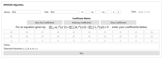
Figure 1. The OPSOLDE Algorithm GUI. Upon inputting an integer value of $n\in [2,9]$, the coefficient field will resize appropriately and permit the user to choose the values for each coefficient. A working example is provided: by selecting “Dirac Coefficients” and the program will generate the results discussed in Section 5.2 of this article.

5. Applications

The simplicity of the above theorems lay in their constructive approach to explicitly computing the polynomial solution coefficients and to provide all the necessary and sufficient conditions for the existence of these polynomials. Further, they can be easily implemented using any available symbolic algebra system. In this section, we show how to make use of these theorems.

5.1. General Case ($n=4$)

To illustrate the constructive approach of Theorem 4, we consider Equation (3) in the case of $n=4$ which reads:

$$\begin{array}{cc}\hfill ({\alpha }_4{r}^4+{\alpha }_3{r}^3+{\alpha }_2{r}^2+{\alpha }_{1}r+{\alpha }_0)y^{″}\left(r\right)+& ({\beta }_3{r}^3+{\beta }_2{r}^2+{\beta }_{1}r+{\beta }_0)y^{\prime }\left(r\right)-({\tau }_2{r}^2+{\tau }_{1}r+{\tau }_0)y\left(r\right)=0,\hfill \\ \hfill & \mathrm{where}{\alpha }_0\ne 0,{\alpha }_k,{\beta }_k,{\tau }_k\in \mathbb{R}\forall k.\hfill \end{array}$$

(58)

For the mth-degree polynomial solutions ${\mathcal{P}}_m\left(r\right)\equiv y\left(r\right)={\sum }_{i=0}^m{\mathcal{C}}_i{r}^i$, (51) gives the five term recurrence-relation:

$$\begin{array}{cc}\hfill [{\alpha }_4& (\ell -2)(\ell -3)+{\beta }_3(\ell -2)-{\tau }_2]{\mathcal{C}}_{\ell -2}+[{\alpha }_3(\ell -1)(\ell -2)+{\beta }_2(\ell -1)-{\tau }_1]{\mathcal{C}}_{\ell -1}\hfill \\ \hfill & +[{\alpha }_2\ell (\ell -1)+{\beta }_1\ell -{\tau }_0]{\mathcal{C}}_{\ell }+[{\alpha }_1(\ell +1)\ell +{\beta }_0(\ell +1)]{\mathcal{C}}_{\ell +1}+\left[{\alpha }_0(\ell +2)(\ell +1)\right]{\mathcal{C}}_{\ell +2}=0,\hfill \end{array}$$

(59)

for $\ell =0,1,2,\dots ,m+2$ and $C_j=0$ for $j<0$.

For the zero-degree ($m=0$) polynomial solution, ${\mathcal{P}}_0\left(r\right)=1$, $\ell =0,1,2$. Noting that ${\mathcal{C}}_j=0$, for all $j\ne 0$, it follows for $\ell =0$ and $\ell =1$ that ${\tau }_0=0$ and ${\tau }_1=0$ respectively, while for $\ell =2$, the necessary condition ${\tau }_2=0$ follows.

For the first-degree ($m=1$) polynomial solution, ${\mathcal{P}}_1\left(r\right)={\mathcal{C}}_0+{\mathcal{C}}_{1}r$, $\ell =0,1,2,3$. Noting that ${\mathcal{C}}_j=0$, for all $j\ne 0,1$, we have for $\ell =0$ that $-{\tau }_0{\mathcal{C}}_0+{\beta }_0{\mathcal{C}}_1=0$, while for $\ell =1$ and $\ell =2$ we have $-{\tau }_1{\mathcal{C}}_0+({\beta }_1-{\tau }_0){\mathcal{C}}_1=0$ and $-{\tau }_2{\mathcal{C}}_0+({\beta }_2-{\tau }_1){\mathcal{C}}_1=0$ respectively. For $\ell =3$ it follows $({\beta }_3-{\tau }_2){\mathcal{C}}_1=0$ from which it is necessary that ${\tau }_2={\beta }_3$, while the first equation ($\ell =0$) gives ${\mathcal{C}}_1={\tau }_0{\mathcal{C}}_0/{\beta }_0$. Using this value for ${\mathcal{C}}_1$ and letting ${\mathcal{C}}_0=1$, the second and third equations ($\ell =1,2$) give $-{\tau }_1{\beta }_0+({\beta }_1-{\tau }_0){\tau }_0=0$ and $-{\tau }_2{\beta }_0+({\beta }_2-{\tau }_1){\tau }_0=0$ respectively. We can write these conditions compactly as:

$$\begin{array}{cc}\hfill & \ell =0:{\mathcal{C}}_1={\tau }_0/{\beta }_0,\hfill \\ \hfill & \ell =1,2:\left\{\begin{array}{c}\left|\begin{array}{cc}-{\tau }_0\hfill & {\beta }_0\hfill \\ -{\tau }_1\hfill & {\beta }_1-{\tau }_0\hfill \end{array}\right|=0,\left(\mathrm{S}1\right)\hfill \\ \hfill \\ \left|\begin{array}{cc}-{\tau }_0\hfill & {\beta }_0\hfill \\ -{\tau }_2\hfill & {\beta }_2-{\tau }_1\hfill \end{array}\right|=0,\left(\mathrm{S}2\right)\hfill \end{array}\right.\hfill \\ \hfill & \ell =3:{\tau }_2={\beta }_3,\left(\mathrm{NC}\right)\hfill \end{array}$$

(60)

where (S1) and (S2) refer to the two sufficient conditions and (NC) refers to the necessary condition.

For the second-degree $(m=2)$ polynomial solution ${\mathcal{P}}_2\left(r\right)=1+{\mathcal{C}}_{1}r+{\mathcal{C}}_2{r}^2$, noting that ${\mathcal{C}}_j=0$, for all $j\ne 0,1,2,$ where $\ell =0,1,2,3,4$ now yields

$$\begin{array}{cc}\hfill & \ell =0,1:\left\{\begin{array}{c}{\mathcal{C}}_1=\frac{\left|\begin{array}{cc}{\tau }_0\hfill & 2{\alpha }_0\hfill \\ {\tau }_1\hfill & 2\left({\alpha }_1+{\beta }_0\right)\hfill \end{array}\right|}{\left|\begin{array}{cc}{\beta }_0\hfill & 2{\alpha }_0\hfill \\ {\beta }_1-{\tau }_0\hfill & 2\left({\alpha }_1+{\beta }_0\right)\hfill \end{array}\right|},\hfill \\ \hfill \\ {\mathcal{C}}_2=\frac{\left|\begin{array}{cc}{\beta }_0\hfill & {\tau }_0\hfill \\ {\beta }_1-{\tau }_0\hfill & {\tau }_1\hfill \end{array}\right|}{\left|\begin{array}{cc}{\beta }_0\hfill & 2{\alpha }_0\hfill \\ {\beta }_1-{\tau }_0\hfill & 2\left({\alpha }_1+{\beta }_0\right)\hfill \end{array}\right|},\hfill \end{array}\right.\hfill \\ \hfill \\ \hfill & \ell =2,3:\left\{\begin{array}{c}\left|\begin{array}{ccc}-{\tau }_0\hfill & {\beta }_0\hfill & 2{\alpha }_0\hfill \\ -{\tau }_1\hfill & {\beta }_1-{\tau }_0\hfill & 2\left({\alpha }_1+{\beta }_0\right)\hfill \\ -{\tau }_2\hfill & {\beta }_2-{\tau }_1\hfill & 2\left({\alpha }_2+{\beta }_1\right)-{\tau }_0\hfill \end{array}\right|=0,\left(\mathrm{S}1\right)\hfill \\ \hfill \\ \left|\begin{array}{ccc}-{\tau }_0\hfill & {\beta }_0\hfill & 2{\alpha }_0\hfill \\ -{\tau }_1\hfill & {\beta }_1-{\tau }_0\hfill & 2\left({\alpha }_1+{\beta }_0\right)\hfill \\ 0\hfill & {\beta }_3-{\tau }_2\hfill & 2\left({\alpha }_3+{\beta }_2\right)-{\tau }_1\hfill \end{array}\right|=0,\left(\mathrm{S}2\right)\hfill \end{array}\right.\hfill \\ \hfill \\ \hfill & \ell =4:2{\alpha }_4+2{\beta }_3-{\tau }_2=0.\left(\mathrm{NC}\right)\hfill \end{array}$$

(61)

For the third degree $(m=3)$ polynomial solution ${\mathcal{P}}_3\left(r\right)=1+{\mathcal{C}}_{1}r+{\mathcal{C}}_2{r}^2+{\mathcal{C}}_3{r}^3$, noting that ${\mathcal{C}}_j=0$, for all $j\ne 0,1,2,3$, we have for $\ell =0,1,2,3,4,5$

$$\begin{array}{cc}\hfill & \ell =0,1,2:\left\{\begin{array}{cc}{\mathcal{C}}_1\hfill & =\frac{\left|\begin{array}{ccc}{\tau }_0\hfill & 2{\alpha }_0\hfill & 0\hfill \\ {\tau }_1\hfill & 2\left({\alpha }_1+{\beta }_0\right)\hfill & 6{\alpha }_0\hfill \\ {\tau }_2\hfill & 2\left({\alpha }_2+{\beta }_1\right)-{\tau }_0\hfill & 3\left(2{\alpha }_1+{\beta }_0\right)\hfill \end{array}\right|}{\left|\begin{array}{ccc}{\beta }_0\hfill & 2{\alpha }_0\hfill & 0\hfill \\ {\beta }_1-{\tau }_0\hfill & 2\left({\alpha }_1+{\beta }_0\right)\hfill & 6{\alpha }_0\hfill \\ {\beta }_2-{\tau }_1\hfill & 2\left({\alpha }_2+{\beta }_1\right)-{\tau }_0\hfill & 3\left(2{\alpha }_1+{\beta }_0\right)\hfill \end{array}\right|},\hfill \\ \\ {\mathcal{C}}_2\hfill & =\frac{\left|\begin{array}{ccc}{\beta }_0\hfill & {\tau }_0\hfill & 0\hfill \\ {\beta }_1-{\tau }_0\hfill & {\tau }_1\hfill & 6{\alpha }_0\hfill \\ {\beta }_2-{\tau }_1\hfill & {\tau }_2\hfill & 3\left(2{\alpha }_1+{\beta }_0\right)\hfill \end{array}\right|}{\left|\begin{array}{ccc}{\beta }_0\hfill & 2{\alpha }_0\hfill & 0\hfill \\ {\beta }_1-{\tau }_0\hfill & 2\left({\alpha }_1+{\beta }_0\right)\hfill & 6{\alpha }_0\hfill \\ {\beta }_2-{\tau }_1\hfill & 2\left({\alpha }_2+{\beta }_1\right)-{\tau }_0\hfill & 3\left(2{\alpha }_1+{\beta }_0\right)\hfill \end{array}\right|},\hfill \\ \\ {\mathcal{C}}_3\hfill & =\frac{\left|\begin{array}{ccc}{\beta }_0\hfill & 2{\alpha }_0\hfill & {\tau }_0\hfill \\ {\beta }_1-{\tau }_0\hfill & 2\left({\alpha }_1+{\beta }_0\right)\hfill & {\tau }_1\hfill \\ {\beta }_2-{\tau }_1\hfill & 2\left({\alpha }_2+{\beta }_1\right)-{\tau }_0\hfill & {\tau }_2\hfill \end{array}\right|}{\left|\begin{array}{ccc}{\beta }_0\hfill & 2{\alpha }_0\hfill & 0\hfill \\ {\beta }_1-{\tau }_0\hfill & 2\left({\alpha }_1+{\beta }_0\right)\hfill & 6{\alpha }_0\hfill \\ {\beta }_2-{\tau }_1\hfill & 2\left({\alpha }_2+{\beta }_1\right)-{\tau }_0\hfill & 3\left(2{\alpha }_1+{\beta }_0\right)\hfill \end{array}\right|},\hfill \end{array}\right.\hfill \end{array}$$

$$\begin{array}{cc}\hfill & \ell =3,4:\left\{\begin{array}{c}\left|\begin{array}{cccc}-{\tau }_0\hfill & {\beta }_0\hfill & 2{\alpha }_0\hfill & 0\hfill \\ -{\tau }_1\hfill & {\beta }_1-{\tau }_0\hfill & 2\left({\alpha }_1+{\beta }_0\right)\hfill & 6{\alpha }_0\hfill \\ -{\tau }_2\hfill & {\beta }_2-{\tau }_1\hfill & 2\left({\alpha }_2+{\beta }_1\right)-{\tau }_0\hfill & 3\left(2{\alpha }_1+{\beta }_0\right)\hfill \\ 0\hfill & {\beta }_3-{\tau }_2\hfill & 2\left({\alpha }_3+{\beta }_2\right)-{\tau }_1\hfill & 6{\alpha }_2+3{\beta }_1-{\tau }_0\hfill \end{array}\right|=0,\left(\mathrm{S}1\right)\hfill \\ \\ \left|\begin{array}{cccc}-{\tau }_0\hfill & {\beta }_0\hfill & 2{\alpha }_0\hfill & 0\hfill \\ -{\tau }_1\hfill & {\beta }_1-{\tau }_0\hfill & 2\left({\alpha }_1+{\beta }_0\right)\hfill & 6{\alpha }_0\hfill \\ -{\tau }_2\hfill & {\beta }_2-{\tau }_1\hfill & 2\left({\alpha }_2+{\beta }_1\right)-{\tau }_0\hfill & 3\left(2{\alpha }_1+{\beta }_0\right)\hfill \\ 0\hfill & 0\hfill & 2\left({\alpha }_4+{\beta }_3\right)-{\tau }_2\hfill & 6{\alpha }_3+3{\beta }_2-{\tau }_1\hfill \end{array}\right|=0,\left(\mathrm{S}2\right)\hfill \end{array}\right.\hfill \end{array}$$

$$\begin{array}{cc}\hfill & \ell =5:6{\alpha }_4+3{\beta }_3-{\tau }_2=0.\left(\mathrm{NC}\right)\hfill \end{array}$$

(62)

Higher-order polynomial solutions may be obtained similarly in this constructive manner.

5.2. Two-Dimensional Dirac Equation

The general covariant $(2+1)$-dimensional Dirac equation reads

$$\begin{array}{c}\hfill i{\gamma }^{\mu }({\partial }_{\mu }+ie{A}_{\mu })\mathsf{\Psi }(t,\overrightarrow{r})=\mathcal{M}\mathsf{\Psi }(t,\overrightarrow{r}),\end{array}$$

(63)

where $\mathcal{M}$ is the rest mass of the particle, $A_{\mu }=(A_0,\overrightarrow{A})$ is the external electromagnetic field potential, and $-e$ is the charge of the particle. Here, ${\gamma }^0={\sigma }_z$, ${\gamma }^1=i{\sigma }_x$, ${\gamma }^2=i{\sigma }_y$, where ${\sigma }_x$, ${\sigma }_y$, and ${\sigma }_z$ are the Pauli spin matrices. Using the generalized momentum operator $P_k=-i{\partial }_k+e{A}_k$ for $k=1,2$ and the conventional summation over $\mu$, Equation (63) may be written in the form

$$\begin{array}{c}\hfill (i{\partial }_t-{\sigma }_x{P}_y+{\sigma }_y{P}_x-{\sigma }_{z}m-e{A}_0)\mathsf{\Psi }(t,\overrightarrow{r})=0.\end{array}$$

(64)

Chiang et al. [16] considered an electron moving in a Coulombic field, $A_0=Ze/r$, with a constant homogeneous magnetic field described by $A_1=-By/2$ and $A_2=Bx/2$. With this choice of potential and for $r>0$, (64) becomes

$$\begin{array}{c}\hfill \left(i{\partial }_t-\left[\begin{array}{cc}\mathcal{M}\hfill & -e^{-i\varphi }({\partial }_r-{\partial }_{\varphi }+\frac{eBr}{2})\hfill \\ e^{i\varphi }({\partial }_r+{\partial }_{\varphi }-\frac{eBr}{2})\hfill & -\mathcal{M}\hfill \end{array}\right]-\frac{Z{e}^2}{r}\right)\mathsf{\Psi }(t,\overrightarrow{r})=0,\end{array}$$

(65)

where polar coordinates, the identities $P_x\pm i{P}_y=-i{e}^{\pm i\varphi }({\partial }_r\pm ({\partial }_{\varphi }-(eBr/2)))$, ${\partial }_x=cos\varphi {\partial }_r-[sin\left(\varphi \right)/r]{\partial }_{\varphi }$, and ${\partial }_y=sin\left(\varphi \right){\partial }_r+[cos\left(\varphi \right)/r]{\partial }_{\varphi }$ were employed [16]. Using separation of variables

$$\begin{array}{c}\hfill \mathsf{\Psi }(t,\overrightarrow{r})=\frac{1}{\sqrt{r}}{e}^{-iEt}\left(\begin{array}{c}F\left(r\right)e^{il\varphi }\hfill \\ G\left(r\right)e^{i(l+1)\varphi }\hfill \end{array}\right),\end{array}$$

(66)

where $l\in \mathbb{Z}$, the Dirac radial Equation (65) reads

$$\begin{array}{cc}\hfill \frac{dF\left(r\right)}{dr}-\left(\frac{l+\frac{1}{2}}{r}+\frac{eB}{2}r\right)F\left(r\right)+\left(E+\mathcal{M}+\frac{Z{e}^2}{r}\right)G\left(r\right)& =0,\hfill \end{array}$$

(67)

$$\begin{array}{cc}\hfill \frac{dG\left(r\right)}{dr}+\left(\frac{l+\frac{1}{2}}{r}+\frac{eB}{2}r\right)G\left(r\right)-\left(E-\mathcal{M}+\frac{Z{e}^2}{r}\right)F\left(r\right)& =0,\hfill \end{array}$$

(68)

For a strong magnetic field, using the asymptotic solutions near $r=0$ and $r=\infty$, it is beneficial to assume an ansatz [16]

$$\begin{array}{cc}\hfill F\left(r\right)& =r^{\gamma }{e}^{-eB{r}^2/4}Q\left(r\right),G\left(r\right)=r^{\gamma }{e}^{-eB{r}^2/4}P\left(r\right),\hfill \end{array}$$

(69)

where $\gamma =\sqrt{{(l+1/2)}^2-{\left(Z{e}^2\right)}^2}$. Substituting (69) into (67) and (68) yields

$$\begin{array}{cc}\hfill & \frac{dQ\left(r\right)}{dr}+\frac{(\gamma -l-\frac{1}{2}-eB{r}^2)}{r}Q\left(r\right)+\left(E+\mathcal{M}+\frac{Z{e}^2}{r}\right)P\left(r\right)=0,\hfill \end{array}$$

(70)

$$\begin{array}{cc}\hfill & \frac{dP\left(r\right)}{dr}+\frac{(\gamma +l+\frac{1}{2})}{r}P\left(r\right)-\left(E-\mathcal{M}+\frac{Z{e}^2}{r}\right)Q\left(r\right)=0.\hfill \end{array}$$

(71)

Solving (70) for $P\left(r\right)$ and substituting the resulting equation into (71) forms a second-order differential equation for $Q\left(r\right)$

$$\begin{array}{cc}\hfill r(r+r_0)Q^{″}\left(r\right)& -(eB{r}^3+eB{r}_0{r}^2-\left(\beta -1\right)r-\beta r_0)Q^{\prime }\left(r\right)\hfill \\ \hfill & +((eB+\epsilon )r^2+(\epsilon r_0+a)r+c-a{r}_0)Q\left(r\right)=0\hfill \end{array}$$

(72)

where $r_0\equiv Z{e}^2/(E+\mathcal{M}),$, $\beta \equiv 2\gamma +1,a\equiv 2EZ{e}^2,\epsilon \equiv E^2-{\mathcal{M}}^2-eB(l+\frac{5}{2}+\gamma ),c\equiv \gamma -l-(1/2).$ Equation (72) is an example of differential equations scattered over a vast range of applications in applied mathematics and theoretical physics [16,17,18,19]. The coefficients ${\left\{{\mathcal{C}}_i\right\}}_{i=0}^m$ of the polynomial solutions $Q_m\left(r\right)={\sum }_{i=0}^m{\mathcal{C}}_i{r}^i$ satisfy the following recurrence relation (53): for $\ell =0,1,\dots ,m+2$

$$\begin{array}{cc}\hfill & \left(E^2-{\mathcal{M}}^2-Be\left(l+\gamma +\ell -\frac{1}{2}\right)\right){\mathcal{C}}_{\ell -2}+\left(Z{e}^2(3E-\mathcal{M})-\frac{B{e}^{3}Z(l+\gamma +\ell +\frac{3}{2})}{E+\mathcal{M}}\right){\mathcal{C}}_{\ell -1}\hfill \\ \hfill & +\left((2\ell +1)\gamma +\ell (\ell -1)-l-\frac{a{e}^{2}Z}{E+\mathcal{M}}-\frac{1}{2}\right){\mathcal{C}}_{\ell }+\frac{e^{2}Z(1+\ell )(1+2\gamma +\ell )}{E+\mathcal{M}}{\mathcal{C}}_{\ell +1}=0.\hfill \end{array}$$

(73)

From Theorem 5, the necessary condition for the polynomial solutions of (72) is

$$\begin{array}{c}\hfill \epsilon =eB(m-1)⟹E_m^2=eB\left(m+l+\gamma +\frac{3}{2}\right)+{\mathcal{M}}^2,m=0,1,\dots .\end{array}$$

(74)

For the zero-degree polynomial solution $Q_0\left(r\right)=1$ where ${\mathcal{C}}_0=1$, $m=0$ and therefore $\ell =0,1,2$, it follows that:

$$\begin{array}{cc}\hfill & \ell =0,1:\left\{\begin{array}{cc}(1+2l-2\gamma )(E+\mathcal{M})+4e^4{Z}^{2}E=0,\hfill & \hfill \left(\mathrm{S}1\right)\\ \hfill \\ eB\left(l+\gamma +\frac{5}{2}\right)-(3E-\mathcal{M})(E+\mathcal{M})=0,\hfill & \hfill \left(\mathrm{S}2\right)\end{array}\right.\hfill \\ \hfill \end{array}$$

$$\begin{array}{cc}\hfill & \ell =2:E^2=Be\left(l+\gamma +\frac{3}{2}\right)+{\mathcal{M}}^2.\left(\mathrm{NC}\right)\hfill \end{array}$$

(75)

For the first-degree polynomial solution $Q_1\left(r\right)=1+{\mathcal{C}}_{1}r$ where ${\mathcal{C}}_0=1$ and ${\mathcal{C}}_1\ne 0$, $m=1$ and therefore $\ell =0,1,2,3$, it follows that:

$$\begin{array}{cc}\hfill & \ell =0:{\mathcal{C}}_1={\displaystyle \frac{(1+2l-2\gamma )(E+\mathcal{M})+4e^{4}E{Z}^2}{2e^{2}Z(1+2\gamma )}},\hfill \\ \hfill & \ell =1,2:\left\{\begin{array}{cc}{e}^{2}Z\left(Be(5+2l+2\gamma )-2(3E-\mathcal{M})(E+\mathcal{M})\right)\hfill & \\ +\left((1+2l-6\gamma )(E+\mathcal{M})+4e^{4}E{Z}^2\right){\mathcal{C}}_1=0,\hfill & \left(\mathrm{S}1\right)\hfill \\ \\ E^2-Be\left(l+\gamma +\frac{3}{2}\right)-{\mathcal{M}}^2\hfill & \\ +\left(e^{2}Z(3E-\mathcal{M})-{\displaystyle \frac{B{e}^{3}Z(l+\gamma +\frac{7}{2})}{E+\mathcal{M}}}\right){\mathcal{C}}_1=0,\hfill & \left(\mathrm{S}2\right)\hfill \end{array}\right.\hfill \\ \hfill & \ell =3:E^2=eB\left(l+\gamma +\frac{5}{2}\right)+{\mathcal{M}}^2.\left(\mathrm{NC}\right)\hfill \end{array}$$

(76)

For the second-degree polynomial solution $Q_2\left(r\right)=1+{\mathcal{C}}_{1}r+{\mathcal{C}}_2{r}^2$ where ${\mathcal{C}}_0=1$ and ${\mathcal{C}}_2\ne 0$, $m=2$ and therefore $\ell =0,1,2,3,4$, it follows that:

$$\begin{array}{cc}\hfill & \ell =0,1:\left\{\begin{array}{c}{\mathcal{C}}_1={\displaystyle \frac{(1+2l-2\gamma )(E+\mathcal{M})+4e^{4}E{Z}^2}{2e^2(1+2\gamma )Z}},\hfill \\ \\ \left(\left(l-3\gamma +\frac{1}{2}\right)(E+\mathcal{M})+2e^4{Z}^{2}E\right){\mathcal{C}}_1-\left(4e^{2}Z(1+\gamma )\right){\mathcal{C}}_2\hfill \\ +e^{2}Z\left(Be\left(l+\gamma +\frac{5}{2}\right)-(3E-\mathcal{M})(E+\mathcal{M})\right)=0,\hfill \end{array}\right.\hfill \end{array}$$

$$\begin{array}{cc}\hfill & \ell =2,3:\left\{\begin{array}{cc}\begin{array}{c}(E+\mathcal{M})\left(E^2-{\mathcal{M}}^2-Be\left(l+\gamma +\frac{3}{2}\right)\right){\mathcal{C}}_0\hfill \\ +e^{2}Z\left((3E-\mathcal{M})(E+\mathcal{M})-Be\left(l+\gamma +\frac{7}{2}\right)\right){\mathcal{C}}_1\hfill \\ +\left(\left(\frac{3}{2}-l+5\gamma \right)(E+\mathcal{M})-2e^{4}E{Z}^2\right){\mathcal{C}}_2=0,\hfill \end{array}\hfill & \left(\mathrm{S}1\right)\hfill \\ \\ \begin{array}{c}\left(E^2-{\mathcal{M}}^2-Be\left(l+\gamma +\frac{5}{2}\right)\right){\mathcal{C}}_1\hfill \\ -{\displaystyle \frac{e^{2}Z\left(Be(l+\gamma +\frac{9}{2})-(3E-\mathcal{M})(E+\mathcal{M})\right)}{E+\mathcal{M}}}{\mathcal{C}}_2=0,\hfill \end{array}\hfill & \left(\mathrm{S}2\right)\hfill \end{array}\right.\hfill \\ \hfill & \ell =4:E^2=eB\left(l+\gamma +\frac{7}{2}\right)+{\mathcal{M}}^2.\left(\mathrm{NC}\right)\hfill \end{array}$$

(77)

Higher-order polynomial solutions follows similarly.

5.3. The Heun Equation

Over the past two decades Heun’s equation has attracted considerable attention due to its increasing number of applications in applied mathematics and theoretical physics [3,4,5,6,7,8,41,42,43,55]. The general second-order Heun differential equation can be written as

$$\left({\alpha }_3{r}^3+{\alpha }_2{r}^2+{\alpha }_{1}r\right)y^{″}\left(r\right)+\left({\beta }_2{r}^2+{\beta }_{1}r+{\beta }_0\right)y^{\prime }\left(r\right)-\left({\tau }_{1}r+{\tau }_0\right)y\left(r\right)=0,$$

(78)

where the canonical form [41] may be obtained using the substitutions given in Table 1.

Table 1. Tabulated values for parameters ${\alpha }_i$, ${\beta }_i$, and ${\tau }_i$ which would transform Equation (78) to the canonical form of the Heun equation.

i	3	2	1	0
${\alpha }_i$	1	$-(c+1)$	c	0
${\beta }_i$		$\delta +ϵ+\gamma$	$-\left(c(\delta +\gamma )+ϵ+\gamma \right)$	$\gamma c$
${\tau }_i$			$-\alpha \beta$	q

We immediately see that because ${\alpha }_0=0$ and ${\alpha }_1\ne 0$ that (78) falls under Theorem 5. By Equation (53) we obtain the three-term recurrence relation

$$\begin{array}{cc}\hfill [{\alpha }_3(\ell +s-2)(\ell +s-1)& +{\beta }_2(\ell +s-1)-{\tau }_1]{\mathcal{C}}_{\ell -1}+\left[{\alpha }_2(\ell +s-1)(\ell +s)+{\beta }_1(\ell +s)-{\tau }_0\right]{\mathcal{C}}_{\ell }\hfill \\ \hfill & +\left[{\alpha }_1(\ell +s)(\ell +s+1)+{\beta }_0(\ell +s+1)\right]{\mathcal{C}}_{\ell +1}=0,\hfill \end{array}$$

(79)

for $\ell =0,1,2,\dots ,m+1$ and $s\in \left\{0,1-({\beta }_0/{\alpha }_1)\right\}$. We may then input this into the Mathematica^® program or work directly with the ($n+2$) equations generated by the recurrence relations (79). Using either approach with $s=0$ will generate the results, as follows.

For the zero-degree ($m=0$) polynomial solution, ${\mathcal{P}}_0\left(r\right)=1$, $\ell =0,1$. Noting that ${\mathcal{C}}_j=0$ for all $j\ne 0$, it follows for $\ell =0$ that ${\tau }_0=0$, while for $\ell =1$, ${\tau }_1=0$.

For the first-degree ($m=1$) polynomial solution, ${\mathcal{P}}_1\left(r\right)={\mathcal{C}}_0+{\mathcal{C}}_{1}r$, $\ell =0,1,2$. It follows that

$$\begin{array}{cc}\hfill \ell & =0:{\mathcal{C}}_1={\tau }_0/{\beta }_0\hfill \\ \hfill \\ \hfill \ell & =1:\left|\begin{array}{cc}-{\tau }_0\hfill & {\beta }_0\hfill \\ -{\tau }_1\hfill & {\beta }_1-{\tau }_0\hfill \end{array}\right|=0,\left(\mathrm{SC}\right)\hfill \\ \hfill \\ \hfill \ell & =2:{\tau }_1={\beta }_2.\left(\mathrm{NC}\right)\hfill \end{array}$$

(80)

where (SC) refers to the sufficient condition and (NC) refers to the necessary condition, and we have set ${\mathcal{C}}_0=1$ for convenience.

For the second-degree $(m=2)$ polynomial solution ${\mathcal{P}}_2\left(r\right)=1+{\mathcal{C}}_{1}r+{\mathcal{C}}_2{r}^2$, $\ell =0,1,2,3$ yields

$$\begin{array}{cc}\hfill & \ell =0,1:\left\{\begin{array}{c}{\mathcal{C}}_1=\frac{\left|\begin{array}{cc}{\tau }_0\hfill & 0\hfill \\ {\tau }_1\hfill & 2\left({\alpha }_1+{\beta }_0\right)\hfill \end{array}\right|}{\left|\begin{array}{cc}{\beta }_0\hfill & 0\hfill \\ {\beta }_1-{\tau }_0\hfill & 2\left({\alpha }_1+{\beta }_0\right)\hfill \end{array}\right|},\hfill \\ \hfill \\ {\mathcal{C}}_2=\frac{\left|\begin{array}{cc}{\beta }_0\hfill & {\tau }_0\hfill \\ {\beta }_1-{\tau }_0\hfill & {\tau }_1\hfill \end{array}\right|}{\left|\begin{array}{cc}{\beta }_0\hfill & 0\hfill \\ {\beta }_1-{\tau }_0\hfill & 2\left({\alpha }_1+{\beta }_0\right)\hfill \end{array}\right|},\hfill \end{array}\right.\hfill \\ \hfill & \ell =2:\left|\begin{array}{ccc}-{\tau }_0\hfill & {\beta }_0\hfill & 0\hfill \\ -{\tau }_1\hfill & {\beta }_1-{\tau }_0\hfill & 2\left({\alpha }_1+{\beta }_0\right)\hfill \\ 0\hfill & {\beta }_2-{\tau }_1\hfill & 2\left({\alpha }_2+{\beta }_1\right)-{\tau }_0\hfill \end{array}\right|=0,\left(\mathrm{SC}\right)\hfill \end{array}$$

$$\begin{array}{cc}\hfill & \ell =3:2{\alpha }_3+2{\beta }_2-{\tau }_1=0.\left(\mathrm{NC}\right)\hfill \end{array}$$

(81)

For the third degree $(m=3)$ polynomial solution ${\mathcal{P}}_3\left(r\right)=1+{\mathcal{C}}_{1}r+{\mathcal{C}}_2{r}^2+{\mathcal{C}}_3{r}^3$. Noting that ${\mathcal{C}}_j=0,$ for all $j\ne 0,1,2$, we have for $\ell =0,1,2,3,4$

$$\begin{array}{c}\hfill \ell =0,1,2:\left\{\begin{array}{cc}{\mathcal{C}}_1\hfill & =\frac{\left|\begin{array}{ccc}{\tau }_0\hfill & 0\hfill & 0\hfill \\ {\tau }_1\hfill & 2\left({\alpha }_1+{\beta }_0\right)\hfill & 0\hfill \\ 0\hfill & 2\left({\alpha }_2+{\beta }_1\right)-{\tau }_0\hfill & 3\left(2{\alpha }_1+{\beta }_0\right)\hfill \end{array}\right|}{\left|\begin{array}{ccc}{\beta }_0\hfill & 0\hfill & 0\hfill \\ {\beta }_1-{\tau }_0\hfill & 2\left({\alpha }_1+{\beta }_0\right)\hfill & 0\hfill \\ {\beta }_2-{\tau }_1\hfill & 2\left({\alpha }_2+{\beta }_1\right)-{\tau }_0\hfill & 3\left(2{\alpha }_1+{\beta }_0\right)\hfill \end{array}\right|},\hfill \\ \\ {\mathcal{C}}_2\hfill & =\frac{\left|\begin{array}{ccc}{\beta }_0\hfill & {\tau }_0\hfill & 0\hfill \\ {\beta }_1-{\tau }_0\hfill & {\tau }_1\hfill & 0\hfill \\ {\beta }_2-{\tau }_1\hfill & 0\hfill & 3\left(2{\alpha }_1+{\beta }_0\right)\hfill \end{array}\right|}{\left|\begin{array}{ccc}{\beta }_0\hfill & 0\hfill & 0\hfill \\ {\beta }_1-{\tau }_0\hfill & 2\left({\alpha }_1+{\beta }_0\right)\hfill & 0\hfill \\ {\beta }_2-{\tau }_1\hfill & 2\left({\alpha }_2+{\beta }_1\right)-{\tau }_0\hfill & 3\left(2{\alpha }_1+{\beta }_0\right)\hfill \end{array}\right|},\hfill \\ \\ {\mathcal{C}}_3\hfill & =\frac{\left|\begin{array}{ccc}{\beta }_0\hfill & 0\hfill & {\tau }_0\hfill \\ {\beta }_1-{\tau }_0\hfill & 2\left({\alpha }_1+{\beta }_0\right)\hfill & {\tau }_1\hfill \\ {\beta }_2-{\tau }_1\hfill & 2\left({\alpha }_2+{\beta }_1\right)-{\tau }_0\hfill & 0\hfill \end{array}\right|}{\left|\begin{array}{ccc}{\beta }_0\hfill & 0\hfill & 0\hfill \\ {\beta }_1-{\tau }_0\hfill & 2\left({\alpha }_1+{\beta }_0\right)\hfill & 0\hfill \\ {\beta }_2-{\tau }_1\hfill & 2\left({\alpha }_2+{\beta }_1\right)-{\tau }_0\hfill & 3\left(2{\alpha }_1+{\beta }_0\right)\hfill \end{array}\right|},\hfill \end{array}\right.\end{array}$$

$$\begin{array}{cc}\hfill & \ell =3:\left|\begin{array}{cccc}-{\tau }_0\hfill & {\beta }_0\hfill & 0\hfill & 0\hfill \\ -{\tau }_1\hfill & {\beta }_1-{\tau }_0\hfill & 2\left({\alpha }_1+{\beta }_0\right)\hfill & 0\hfill \\ 0\hfill & {\beta }_2-{\tau }_1\hfill & 2\left({\alpha }_2+{\beta }_1\right)-{\tau }_0\hfill & 3\left(2{\alpha }_1+{\beta }_0\right)\hfill \\ 0\hfill & 0\hfill & 2\left({\alpha }_3+{\beta }_2\right)-{\tau }_1\hfill & 6{\alpha }_2+3{\beta }_1-{\tau }_0\hfill \end{array}\right|=0,\left(\mathrm{SC}\right)\hfill \\ \hfill \\ \hfill & \ell =4:6{\alpha }_3+3{\beta }_2-{\tau }_1=0.\left(\mathrm{NC}\right)\hfill \end{array}$$

(82)

This approach allows us to construct all the Heun polynomial solutions in a constructive way that is not available in the literature.

6. Conclusions

Given a linear differential equation with polynomial coefficients of order n, $n-1$, and $n-2$ respectively, this work provides a constructive and straightforward approach for finding all possible polynomial solutions along with the necessary and sufficient conditions. A Mathematica program which solves these differential equations for an integer value of $n\in [2,9]$ is available for download (see Section 4.2), but the algorithms are also provided so that the reader may adopt them in their preferred computer software. Although there may be other sophisticated approaches available in the literature for solving differential equations [46], the method presented here has its simplicity characterized by recurrence relations. Aside from the examples discussed in this present work, the authors explored a large number of linear differential equations which appeared in mathematics and physics literature, and have found exact consistency with the results obtained by other researchers [3,4,5,6,7,8,9,10,43,55].

References

- Primitivo, B. Acosta-Humánez, David Blázquez-Sanz, Henock Venegas-Gómez, Liouvillian solutions for second order linear differential equations with polynomial coefficients. São Paulo J. Math. Sci. 2020. [Google Scholar] [CrossRef]
- Raposo, A.P.; Weber, H.J.; Alvarez-Castillo, D.E.; Kirchbach, M. Romanovski polynomials in selected physics problems. Centr. Eur. J. Phys. 2007, 5, 253–284. [Google Scholar] [CrossRef]
- Ovsiyuk, E.; Amirfachrian, M.; Veko, O. On Schrödinger equation with potential V(r)=αr−1+βr+kr2 and the biconfluent Heun functions theory. Nonl. Phen. Compl. Sys. 2012, 15, 163. [Google Scholar]
- Caruso, F.; Martins, J.; Oguri, V. Solving a two-electron quantum dot model in terms of polynomial solutions of a biconfluent Heun equation. Ann. Phys. 2014, 347, 130–140. [Google Scholar] [CrossRef]
- Marcilhacy, G.; Pons, R. The Schrödinger equation for the interaction potential x2 + λx2/(1 + gx2), and the first Heun confluent equation. J. Phys. A Math. Gen. 1985, 18, 2441–2449. [Google Scholar] [CrossRef]
- Exton, H. The interaction V(r) = −Ze2/(r + β) and the confluent Heun equation. J. Phys. A Math. Gen. 1991, 24, L329–L330. [Google Scholar] [CrossRef]
- Ciftci, H.; Hall, R.L.; Saad, N.; Dogu, E. Physical applications of second-order linear differential equations that admit polynomial solutions. J. Phys. A Math. Theor. 2010, 43, 415206. [Google Scholar] [CrossRef]
- Hall, R.H.; Saad, N.; Sen, K.D. Soft-core Coulomb potentials and Heun’s differential equation. J. Math. Phys. 2010, 51, 022107. [Google Scholar] [CrossRef]
- Hall, R.L.; Saad, N.; Sen, K.D. Discrete spectra for confined and unconfined −a/r + br2 potentials in d-dimensions. J. Math. Phys. 2011, 52, 092103. [Google Scholar] [CrossRef]
- Hall, R.L.; Saad, N.; Sen, K.D. Spectral characteristics for a spherically confined −a/r + br2 potential. J. Phys. A Math. Theor. 2011, 44, 185307. [Google Scholar] [CrossRef]
- Hortacsu, M. Heun functions and their uses in physics. arXiv 2013, arXiv:1101.0471v1. [Google Scholar]
- Zhang, Y.-Z. Exact polynomial solutions of second order differential equations and their applications. J. Phys. A Math. Theor. 2012, 45, 065206. [Google Scholar] [CrossRef]
- Saad, N.; Hall, R.L.; Trenton, V. Polynomial solutions for a class of second-order linear differential equations. Appl. Math. Comput. 2014, 226, 615–634. [Google Scholar] [CrossRef][Green Version]
- Wen, F.-K.; Yang, Z.-Y.; Liu, C.; Yang, W.-L.; Zhang, Y.-Z. Exact polynomial solutions of Schrödinger equation with various hyperbolic potentials. Commun. Theor. Phys. 2014, 61, 153. [Google Scholar] [CrossRef]
- Sun, D.; You, Y.; Lu, F.; Chen, C.; Dong, S. The quantum characteristics of a class of complicated double ring-shaped non-central potential. Phys. Scr. 2014, 89, 045002. [Google Scholar] [CrossRef]
- Chiang, C.; Ho, C. Planar Dirac electron in Coulomb and magnetic fields: A Bethe ansatz approach. J. Math. Phys. 2002, 43, 43–51. [Google Scholar] [CrossRef]
- Chen, C.Y.; Lu, F.L.; Sun, D.S.; Dong, S.H. The origin and mathematical characteristics of the Super-Universal Associated-Legendre polynomials. Commun. Theor. Phys. 2014, 62, 331–337. [Google Scholar] [CrossRef]
- Chen, C.Y.; You, Y.; Lu, F.L.; Sun, D.S.; Dong, S.-H. Exact solutions to a class of differential equation and some new mathematical properties for the universal associated-Legendre polynomials. Appl. Math. Lett. 2015, 40, 90–96. [Google Scholar] [CrossRef]
- Chen, C.Y.; Lu, F.L.; Sun, D.S.; You, Y.; Dong, S.-H. Spin-orbit interaction for the double ring-shaped oscillator. Ann. Phys. 2016, 371, 183–198. [Google Scholar] [CrossRef]
- Dong, S.; Sun, G.; Falaye, B.J.; Dong, S.-H. Semi-exact solutions to position-dependent mass Schrödinger problem with a class of hyperbolic potential V0 tanh(ax). Eur. Phys. J. Plus 2016, 131, 176. [Google Scholar] [CrossRef]
- Ishkhanyan, A. Exact solution of the Schrödinger equation for the inverse square root potential. Europhys. Lett. 2015, 112, 10006. [Google Scholar] [CrossRef]
- Li, W.; Dai, W. Exact solution of inverse-square-root potential V(x) = −α/r. Ann. Phys. 2016, 373, 207–215. [Google Scholar] [CrossRef]
- Fernández, F.M. Comment on: Exact solution of the inverse-square-root potential V(r)=−α/r. Ann. Phys. 2017, 379, 83–85. [Google Scholar] [CrossRef]
- Ishkhanyan, A.M. Schrödinger potentials solvable in terms of the general Heun functions. Ann. Phys. 2018, 388, 456–471. [Google Scholar] [CrossRef]
- Ishkhanyan, A.M. Exact solution of the Schrödinger equation for a short-range exponential potential with inverse square root singularity. Eur. Phys. J. Plus 2018, 133, 83. [Google Scholar] [CrossRef]
- Maiz, F.; Alqahtani, M.M.; Al Sdran, N.; Ghnaim, I. Sextic and decatic anharmonic oscillator potentials: Polynomial solutions. Phys. B 2018, 530, 101–106. [Google Scholar] [CrossRef]
- Dong, S.; Dong, Q.; Sun, G.-H.; Femmam, S.; Dong, S.-H. Exact solutions of the Razavy Cosine Type potential. Adv. High Energy Phys. 2018, 2018, 5824271. [Google Scholar]
- Dong, Q.; Serrano, F.A.; Sun, G.-H.; Jing, J.; Dong, S.-H. Semi-exact Solutions of the Razavy Potential. Adv. High Energy Phys. 2018, 2018, 9105825. [Google Scholar] [CrossRef]
- Dong, Q.; Dong, S.S.; Hernández-Márquez, E.; Silva-Ortigoza, R.; Sun, G.H.; Dong, S.H. Semi-exact Solutions of Konwent Potential. Commun. Theor. Phys. 2019, 71, 231. [Google Scholar] [CrossRef]
- Dong, Q.; Sun, G.-H.; Jing, J.; Dong, S.-H. New findings for two new type sine hyperbolic potentials. Phys. Lett. A 2019, 383, 270–275. [Google Scholar] [CrossRef]
- Bazighifan, O. Some New Oscillation Results for Fourth-Order Neutral Differential Equations with a Canonical Operator. Math. Probl. Eng. 2020. [Google Scholar] [CrossRef]
- Agarwal, R.P.; Zhang, C.; Li, T. Some remarks on oscillation of second order neutral differential equations. Appl. Math. Comput. 2016, 274, 178–181. [Google Scholar]
- Euler, L. Institutiones Calculi Integralis, Vol. 2; Opera Omnia I: St. Petersburg, Russia, 1769; pp. 221–230. [Google Scholar]
- Scheffé, H. Linear differential equations with two-term recurrence formulas. J. Math. Phys. 1941, 21, 240–249. [Google Scholar] [CrossRef]
- Shore, S.D. On the second order differential equation which has orthogonal polynomial solutions. Bull. Calcutta Math. Soc. 1964, 56, 195–198. [Google Scholar]
- Hahn, W. On differential equations for orthogonal polynomials. Funkcialaj Ekuacioj 1978, 21, 1–9. [Google Scholar]
- Littlejohn, L.; Shore, S. Nonclassical orthogonal polynomials as solutions to second-order differential equations. Can. Math. Bull. 1982, 25, 291–295. [Google Scholar] [CrossRef]
- Littlejohn, L. On the classification of differential equations having orthogonal polynomial solutions. Ann. Mat. Pura Appl. 1984, 138, 35–53. [Google Scholar] [CrossRef]
- Al-Salam, W.A. Characterization Theorems for orthogonal polynomials. In Orthogonal Polynomials: Theory and Practice; Paul, N., Ed.; Springer: Dordrecht, The Netherlands, 1990. [Google Scholar]
- Atakishiyev, N.M.; Rahman, M.; Suslov, S.K. On classical orthogonal polynomials. Constr. Approx. 1995, 11, 181–226. [Google Scholar] [CrossRef]
- Ronveaux, A. Heun’s Differential Equation; Oxford University Press: Oxford, UK, 1995. [Google Scholar]
- Maier, R.S. The 192 solutions of the Heun equation. Math. Comput. 2007, 76, 811–843. [Google Scholar] [CrossRef]
- El-Jaick, L.J.; Bartolomeu, D.B.; Figueiredo, D.B. On certain solutions for confluent and double-confluent Heun equations. J. Math. Phys. 2008, 49, 082508. [Google Scholar] [CrossRef]
- Kwon, K.H.; Littlejohn, L.L. Sobolev orthogonal polynomials and second-order differential equations. Rocky Mt. J. Math. 1998, 28, 547–594. [Google Scholar] [CrossRef]
- Everitt, W.N.; Kwon, K.H.; Littlejohn, L.L.; Wellman, R. Orthogonal polynomial solutions of linear ordinary differential equations. J. Comput. Appl. Math. 2001, 133, 85–109. [Google Scholar] [CrossRef]
- Bluman, G.; Dridi, R. New solutions for ordinary differential equations. J. Symb. Comput. 2012, 47, 76–88. [Google Scholar] [CrossRef][Green Version]
- Routh, E.J. On some properties of certain solutions of a differential equation of the second order. Proc. Lond. Math. Soc. 1884, 1, 245–262. [Google Scholar] [CrossRef]
- Bochner, S. Über Sturm-Liouvillesche Polynomsysteme. Math. Z. 1929, 29, 730–736. [Google Scholar] [CrossRef]
- Slavyanov, S.Y.; Lay, W. Special Functions, A Unified Theory Based on Singularities; Oxford Mathematical Monographs: Oxford, UK, 2000. [Google Scholar]
- Ince, E.L. Ordinary Differential Equations; Dover Publications: Mineola, NY, USA, 1956. [Google Scholar]
- Forsyth, A.R. A Treatise on Differential Equations, 6th ed.; Macmillan: London, UK, 1933. [Google Scholar]
- Ciftci, H.; Hall, R.L.; Saad, N. Asymptotic iteration method for eigenvalue problems. J. Phys. A Math. Gen. 2003, 36, 11807–11816. [Google Scholar] [CrossRef]
- Saad, N.; Hall, R.L.; Ciftci, H. Criterion for polynomial solutions to a class of linear differential equations of second order. J. Phys. A Math. Gen. 2005, 38, 1147. [Google Scholar] [CrossRef]
- Dong, S.-H. Wave Equations in Higher Dimensions; Springer: Dordrecht, The Netherlands, 2011. [Google Scholar]
- Rovder, J. Zeros of the polynomial solutions of the differential equation xy″ + (β0 + β1x + β2x2)y′ + (γ−nβ2x)y = 0. Mat. Căs. 1974, 24, 15. [Google Scholar]
Publisher’s Note: MDPI stays neutral with regard to jurisdictional claims in published maps and institutional affiliations. |
© 2020 by the authors. Licensee MDPI, Basel, Switzerland. This article is an open access article distributed under the terms and conditions of the Creative Commons Attribution (CC BY) license (http://creativecommons.org/licenses/by/4.0/).