Self-Learning Salp Swarm Optimization Based PID Design of Doha RO Plant

Abstract

In this investigation, self-learning salp swarm optimization (SLSSO) based proportional- integral-derivative (PID) controllers are proposed for a Doha reverse osmosis desalination plant. Since the Doha reverse osmosis plant (DROP) is interacting with a two-input-two-output (TITO) system, a decoupler is designed to nullify the interaction dynamics. Once the decoupler is designed properly, two PID controllers are tuned for two non-interacting loops by minimizing the integral-square-error (ISE). The ISEs for two loops are obtained in terms of alpha and beta parameters to simplify the simulation. Thus designed ISEs are minimized using SLSSO algorithm. In order to show the effectiveness of the proposed algorithm, the controller tuning is also accomplished using some state-of-the-art algorithms. Further, statistical analysis is presented to prove the effectiveness of SLSSO. In addition, the time domain specifications are presented for different test cases. The step responses are also shown for fixed and variable reference inputs for two loops. The quantitative and qualitative results presented show the effectiveness of SLSSO for the DROP system.

1. Introduction

The existence of civilization depends upon the availability of potable water. The studies are repeatedly indicating that the potable water is acutely depleted in the last few decades. The main reason for depletion of fresh water is overuse of ground water due to growing population and industrialization [1]. In order to meet the requirements due to increased population and industrialization, it is required to explore for sources of fresh water. The desalination of sea water is one of the possible solutions since the expense of sea water is abundant [2].

The process of removing salts from saline water is called desalination [3]. Desalination is achieved by (a) thermal distillation processes such as multiple effect evaporation, multi-stage flash (MSF), vapour compression, etc., and (b) membrane processes such as nano-filtration, electro-dialysis reversal, forward osmosis, reverse osmosis (RO), etc. Among these, RO has been proved to be economical [4]. RO process also produces high quality water with minimal energy consumption. Additionally, there is low initial investment in case of RO process.

RO is a filtration process which segregates fresh water from higher concentrated saline water. In RO process, a semi-permeable membrane is used which passes the fresh water through it and rejects the concentrated solution. The various plants which use the RO process are Doha RO system [5], Chaabene RO system [6], Riverol and Pilipovik [7], etc. The various pilot-scale models [8] for RO are also presented in literature. The RO models given in literature are interacting having flux and conductivity as controlled variables generally.

The most common controller used for interacting RO models is a proportional-integral-derivative (PID) controller. The PID controller is used due to its simple structure and being able to produce satisfactory performance. The performance of PID controller depends on the quality of tuning. The classical methods [9] used for tuning are Ziegler–Nichols, gain-phase margin method, Cohen–Coon, etc. However, the main drawback with classical tuning methods is moderate performance of the controller [10]. The controller performance can be enhanced by improving the quality of tuning.

Various optimization based methods can guarantee the improved quality of tuning [11]. Recently, the intelligent optimization algorithms like fireworks algorithm [12], bacterial foraging optimization [13], elephant herding optimization [10], whale optimization algorithm [2,14], monarch butterfly optimization [15], brain storm optimization [16], etc. are proposed in the existing literature. Some techniques are proposed in the literature for tuning the PID controller for RO systems. In [11], PID controller is designed using Luus–Jaakola (LJ) optimization algorithm for the RO system. Particle swarm optimization (PSO) is utilized for tuning the PID controller parameters in [17].

Grey wolf optimization (GWO) assisted PID tuning for RO system is presented in [4]. Similarly, whale optimization algorithm and elephant herding optimization based controllers are suggested in [2,10], respectively. Other relevant controller designs can be found in [18,19]. The methods presented in [2,4,10,19] also provide better response when compared to classical methods of tuning of PID controller. However, the methods proposed in [2,4,10,19] are providing the tuning with basic algorithms only. It is well known that the basic algorithms have the problem of local minima trapping [20]. So sometimes, it becomes necessary to enhance the performance of basic algorithm by some modifications [21,22].

In this investigation, an improved algorithm, i.e., self learning salp swarm optimization (SLSSO), is utilized for tuning of PID controllers [23]. The controller tuning is presented for Doha reverse osmosis plant (DROP). DROP model is having two controlled variables namely, flux and conductivity and two manipulated variables namely, pressure and pH. These four variables are interacting in nature. This makes DROP model an interacting two-input-two-output (TITO) system. 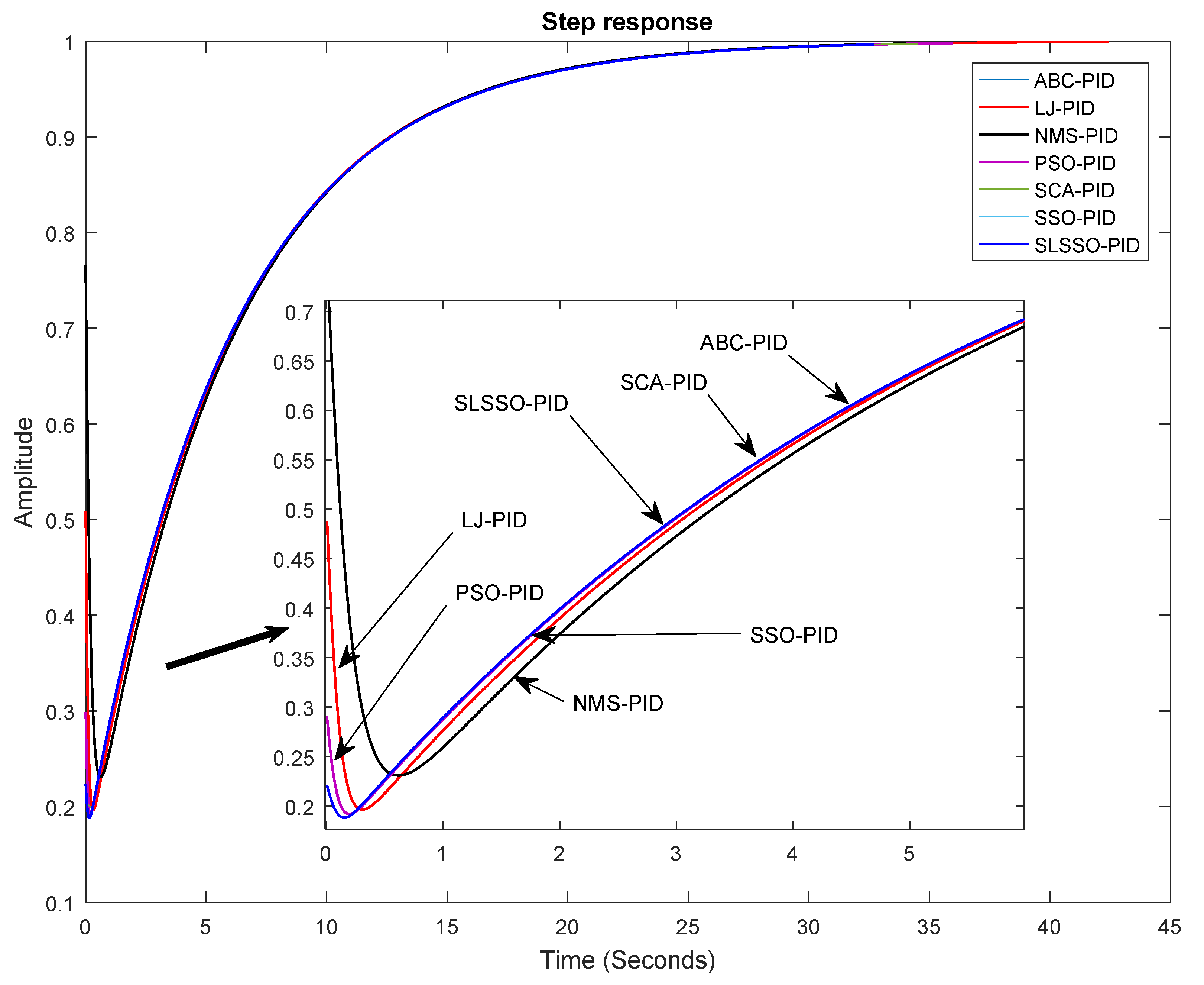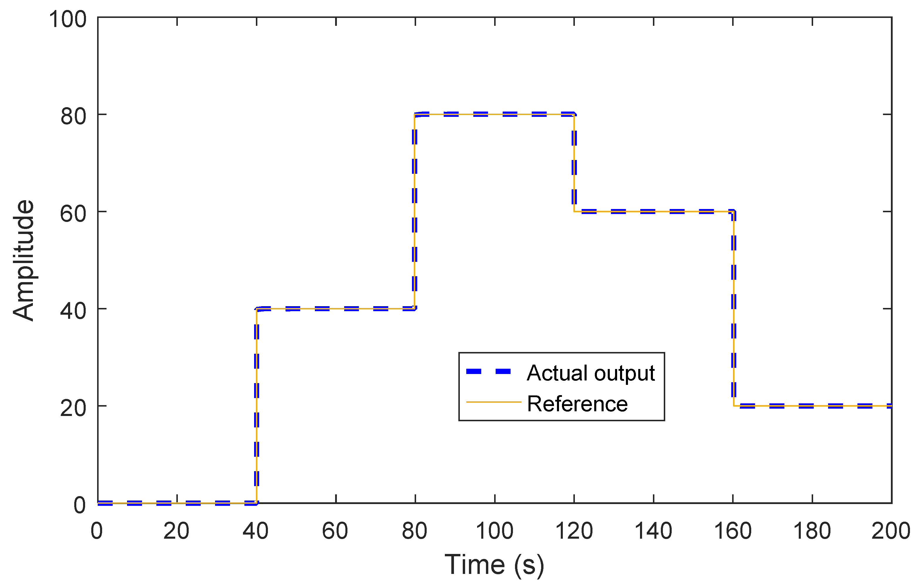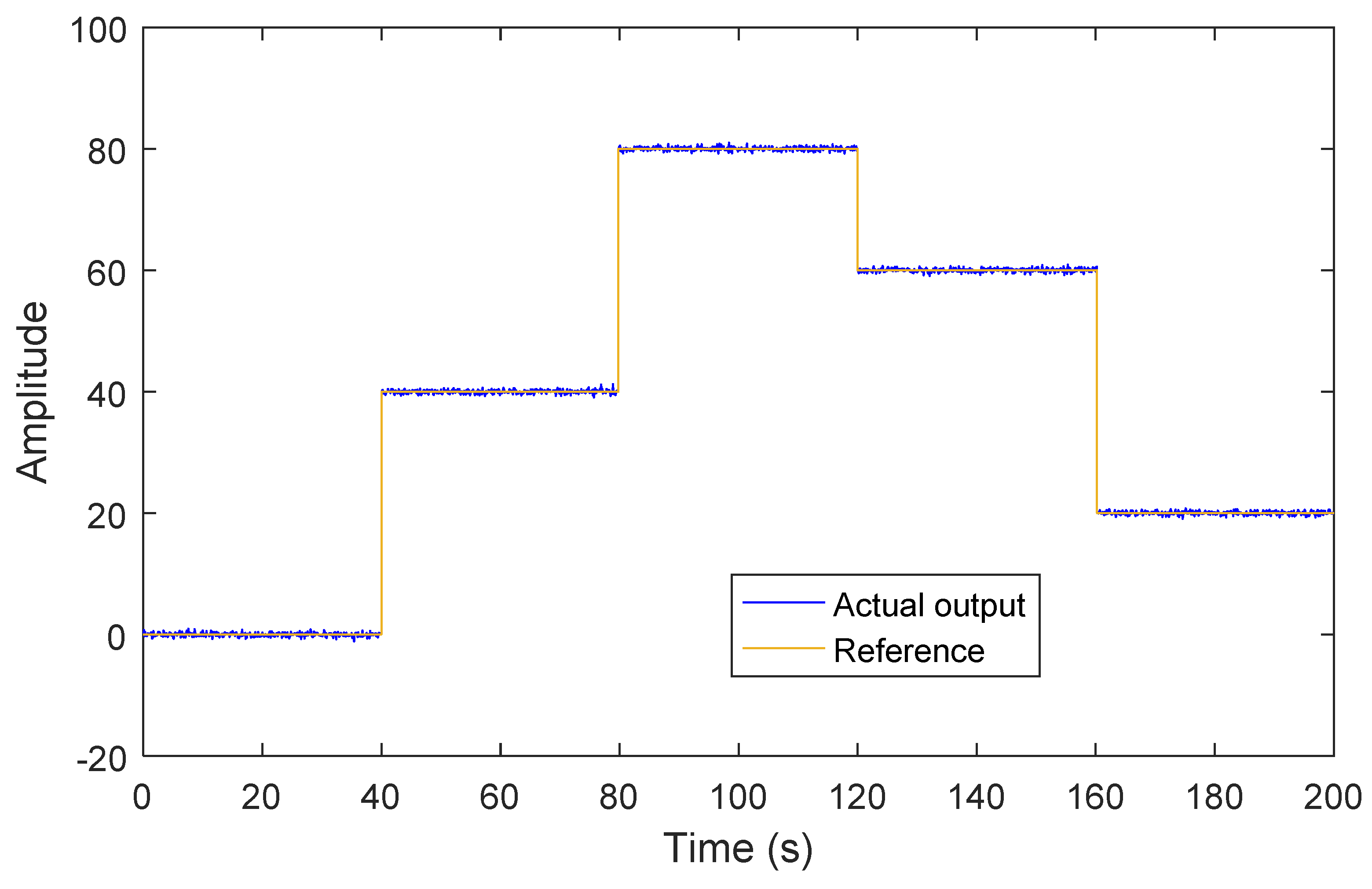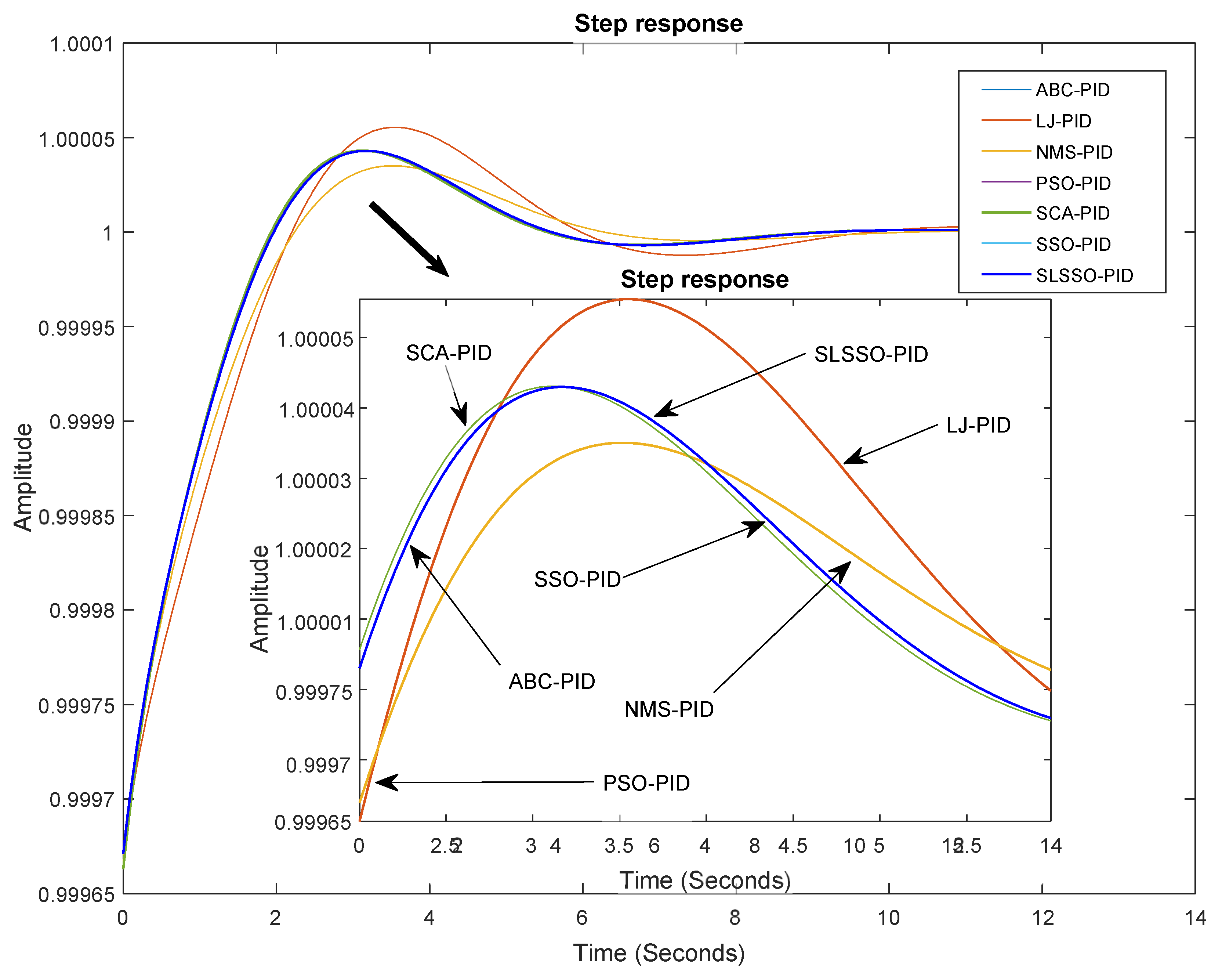First, a decoupler is designed using feed-forward method [24] of decoupling to make the system non-interacting in nature. Thus obtained model has two non-interacting loops, one for flux and other for conductivity. Then, two PID controllers are obtained for two non-interacting loops using SLSSO algorithm. The integral-of-squared-error (ISE) is taken as tuning criterion. For the ease of simulation, the ISE is formulated in terms of alpha and beta parameters. The key features of proposed method are: (a) it is utilizing SLSSO for tuning of PID controllers, (b) a decoupler is designed for interacting Doha RO system, (c) the ISE is formulated in terms of alpha and beta parameters, and (d) the results of SLSSO are also compared with other algorithms to prove its supremacy. This study also obtained the PID controllers using artificial bee colony (ABC) algorithm, LJ algorithm, Nelder–Mead simplex (NMS) algorithm, sine cosine algorithm (SCA) and salp swarm optimization (SSO) algorithm for fair comparisons of performance of SLSSO tuned controllers. Additionally, time-domain specifications are tabulated for comparisons. Further, the statistical analysis of ISE obtained for controllers is presented. Moreover, the closed-loop responses (step, impulse and variable step responses) are also shown for different controllers.

The structure of the paper is as follows: Section 2 presents the description of reverse osmosis system in consideration. The interacting TITO system is given in the same section. In addition, the decoupler design is described in this section. The controller structure is presented in Section 3. Section 4 is presenting the SSO algorithm. The description of SLSSO algorithm is also given in the same section. Section 5 presents results and discussion where two case studies are discussed in detail. Finally, the findings of paper are concluded in Section 6.

2. Reverse Osmosis System

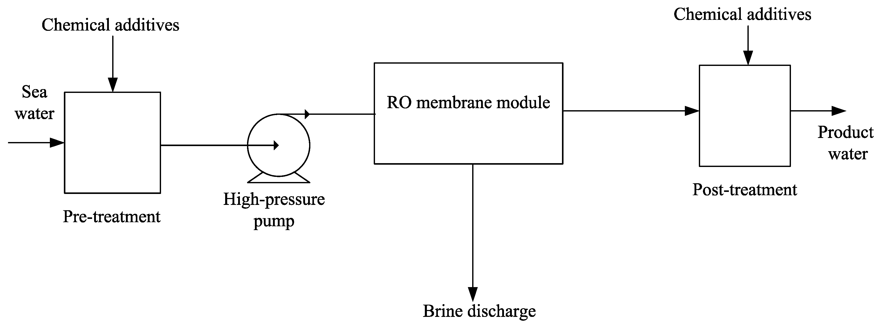
The schematic block diagram of Doha reverse osmosis plant (DROP) system is provided in Figure 1 [4]. The RO desalination plant comprises of four stages, namely, pre-treatment, high pressure pump, RO membrane assembly and post-treatment.

During pre-treatment stage, the saline water undergoes filtration to remove any physical or chemical impurities. This stage is important to ensure membrane longevity. The organic chemicals which can burn holes in the membrane and can cause irreparable damage to membrane are trapped using activated cartridge filters. In addition, some inhibitors are added to decrease the pH of the feed-water which helps in reducing the scaling effect. Besides this, physical impurities like mud particles and microbial growth on membrane are also removed during this stage to increase the life of membrane.

High pressure pump is utilized to provide the necessary pressure required for reverse osmosis. For brackish water, it is in the range of 15–25 bars while it is 54–80 bars for sea water. The pressurized feed-water is then fed to the membrane assembly which is made up of two or more hollow or spiral wound composite polyamide membranes. This is the main part of the RO system. It does not allow impurities to pass through it. The membrane assembly must be able to withstand the high pressure. The rejected brine from membrane assembly is sent to the discharge channel. In post-treatment stage, calcium and bi-carbonate ions are removed from the water. In addition, the pH is raised slightly above 7 and water is prepared for distribution. The two controlled variables (flux and conductivity of output water) are manipulated using two manipulated variables (feed-water pressure and feed-water pH) in case of DROP model.

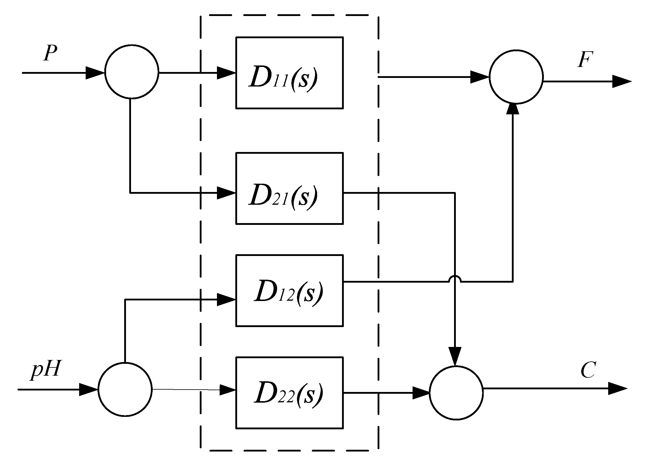
2.1. Control-Loops for DROP Model

The block diagram of DROP is given in Figure 2. The transfer function of interacting DROP model is given as

$$\left[\begin{array}{c}{Y}_1\left(s\right)\\ Y_2\left(s\right)\end{array}\right]=\left[\begin{array}{cc}{D}_{11}\left(s\right)& D_{12}\left(s\right)\\ D_{21}\left(s\right)& D_{22}\left(s\right)\end{array}\right]\left[\begin{array}{c}{R}_1\left(s\right)\\ R_2\left(s\right)\end{array}\right]$$

(1)

where $R_1\left(s\right)$ and $R_2\left(s\right)$ are two manipulated variables which are feed-water pressure and feed-water pH, respectively, and $Y_1\left(s\right)$ and $Y_2\left(s\right)$ are two controlled variables which are flow and conductivity of output water, respectively. The transfer functions $D_{11}\left(s\right)$, $D_{12}\left(s\right)$, $D_{21}\left(s\right)$ and $D_{22}\left(s\right)$ are denoting the individual transfer functions in between two manipulated variables and two controlled variables.

The transfer functions $D_{11}\left(s\right)$, $D_{12}\left(s\right)$, $D_{21}\left(s\right)$ and $D_{22}\left(s\right)$ are given as:

$$D_{11}\left(s\right)=\frac{k_{11}(n_{11}s+1)}{s^2+2{\zeta }_{11}{d}_{11}s+d_{11}}$$

(2)

$$D_{12}\left(s\right)=0$$

(3)

$$D_{21}\left(s\right)=\frac{k_{21}(n_{21}s+1)}{s^2+2{\zeta }_{21}{d}_{11}s+d_{21}}$$

(4)

$$D_{22}\left(s\right)=\frac{k_{22}(n_{22}s+1)}{s^2+2{\zeta }_{22}{d}_{22}s+d_{22}}$$

(5)

It can easily be concluded from transfer functions (2)–(5) that both flow and conductivity are manipulated by feed-water pressure. However, the feed-water pH is affecting only conductivity. The values of different parameters of transfer functions (2)–(5), are given in

Table 1. Parameters at salinity of 3000 μS/cm.

Parameter	${\mathit{k}}_{11}$	${\mathit{n}}_{11}$	${\mathit{\zeta }}_{11}$	${\mathit{d}}_{11}$	${\mathit{k}}_{21}$	${\mathit{n}}_{21}$	${\mathit{\zeta }}_{21}$	${\mathit{d}}_{21}$	${\mathit{k}}_{22}$	${\mathit{n}}_{22}$	${\mathit{\zeta }}_{22}$	${\mathit{d}}_{22}$
Value	$0.67$	$0.056$	$0.91$	$18.26$	$-2.39$	$0.35$	$0.76$	$2.17$	$-95$	$0.32$	$1.16$	$1.29$

[4]. The interval transfer functions of (2)–(5) turn out to be (2)–(5) by considering 40% uncertainty.

$$\begin{array}{c}\hfill D_{11}\left(s\right)={\displaystyle \frac{\left[0.402,0.938\right]+\left[0.0225,0.0525\right]s}{\left[10.956,25.564\right]+\left[19.938,46.522\right]s+\left[0.60,1.40\right]s^2}}\end{array}$$

(6)

$$\begin{array}{c}\hfill D_{12}\left(s\right)=0\end{array}$$

(7)

$$\begin{array}{c}\hfill D_{21}\left(s\right)={\displaystyle \frac{\left[-3.346,-1.434\right]+\left[-1.1711,-0.5019\right]s}{\left[1.302,3.038\right]+\left[16.65,38.85\right]s+\left[0.60,1.40\right]s^2}}\end{array}$$

(8)

$$\begin{array}{c}\hfill D_{22}\left(s\right)={\displaystyle \frac{\left[-113,-57\right]+\left[-42.63,-18.27\right]s}{\left[0.774,1.806\right]+\left[1.794,4.186\right]s+\left[0.60,1.40\right]s^2}}\end{array}$$

(9)

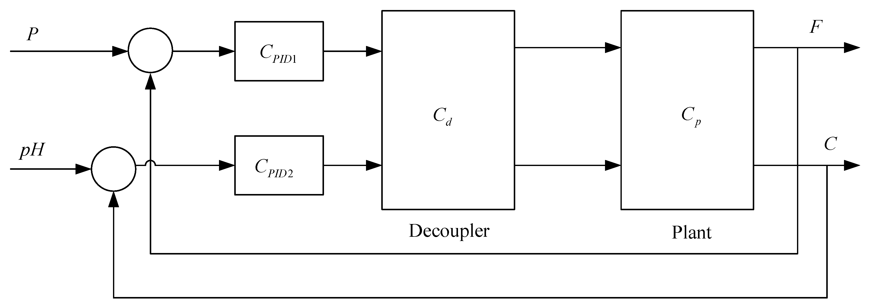
2.2. Design of Decoupler

A decoupler is required to be designed to nullify the effect of interaction for interacting TITO system. Figure 3 shows the decoupler along with the plant. This work employs simplified decoupling technique [17] to convert interacting TITO system into two non-interacting control loops. The transfer function of decoupler is obtained by

$$T=C_p{C}_d$$

(10)

such that

$$T=\left[\begin{array}{cc}{T}_{11}\left(s\right)& 0\\ 0& T_{22}\left(s\right)\end{array}\right]$$

(11)

$$C_d=\left[\begin{array}{cc}1& x\\ y& 1\end{array}\right]$$

(12)

where $C_p$ and $C_d$ are, respectively, the transfer functions of plant and decoupler. From (10), it is obtained

$$x=-\frac{D_{12}\left(s\right)}{D_{22}\left(s\right)}$$

(13)

$$y=-\frac{D_{21}\left(s\right)}{D_{11}\left(s\right)}$$

(14)

$$T_{11}=\frac{D_{11}\left(s\right)D_{22}\left(s\right)-D_{12}\left(s\right)D_{21}\left(s\right)}{D_{22}\left(s\right)}$$

(15)

$$T_{22}=\frac{D_{11}\left(s\right)D_{22}\left(s\right)-D_{12}\left(s\right)D_{21}\left(s\right)}{D_{11}\left(s\right)}$$

(16)

Hence, it is clear from (13)–(16) that by choosing x and y as given in (13) and (14), respectively, the interacting system is decoupled into two non-interacting loops with transfer functions, $T_{11}$ and $T_{22}$ as given in (15) and (16), respectively. Thus, two independent PID controllers, $C_{PID1}$ and $C_{PID2}$, can be obtained for two non-interacting loops having transfer functions, namely $T_{11}$ and $T_{22}$ .

3. Controller Design

3.1. Controller Structure

In literature, many structures of PID controller are existing. However, the simple and widely used parallel form given in (17) is used in this work.

$$u\left(t\right)=K_{p}e\left(t\right)+K_i{\int }_0^{t}e\left(t\right)dt+K_{d}e\left(t\right)$$

(17)

The parameters, $K_p$, $K_i$ and $K_d$ are, respectively, the proportional, integral and derivative gains. However, $u\left(t\right)$ and $e\left(t\right)$ denote the control effort generated by controller and error signal fed to controller, respectively. In Laplace domain, (17) becomes as given in (18).

$$C_{PID}=\frac{U\left(s\right)}{E\left(s\right)}=K_p+\frac{K_i}{s}+K_{d}s$$

(18)

3.2. The Determination of ISEs for DOHA Plant

The ISE is utilized for obtaining the controller parameters. The ISE is obtained in terms of alpha and beta parameters. The ISE for two independent loops, i.e., pressure-flux and pH-conductivity loops, is given below.

(a)

ISE for pressure-flux loop:

$$IS{E}_1={\int }_0^{\infty }{e}_1^2\left(t\right)dt=\sum _{i=1}^k\frac{{\beta }_i^2}{2{\alpha }_i}$$

(19)

(b)

ISE for pH-conductivity loop:

$$IS{E}_2={\int }_0^{\infty }{e}_2^2\left(t\right)dt=\sum _{i=1}^{\overline{k}}\frac{{\overline{\beta }}_i^2}{2{\overline{\alpha }}_i}$$

(20)

The alpha and beta parameters are obtained utilizing alpha and beta tables. The alpha and beta tables are derived from respective error in Laplace domain. Suppose the error in Laplace domain is given as

$$E\left(s\right)=\frac{U_{m-1}{s}^{m-1}+\cdots +U_{1}s+U_0}{V_m{s}^m+V_{m-1}{s}^{m-1}+\cdots +V_{1}s+V_0}$$

(21)

The alpha and beta tables are constructed as given in

Table 2. Alpha table.

	$c_0^0=V_m$	$c_2^0=V_{m-2}$	$c_4^0=V_{m-4}$	$c_6^0=V_{m-6}$
	$c_1^0=V_{m-1}$	$c_2^1=V_{m-3}$	$c_4^1=V_{m-5}$	⋯
${\alpha }_1$=$c_0^0$/$c_0^1$	$c_0^2=c_2^0-{\alpha }_1{c}_2^1$	$c_2^2=c_4^0-{\alpha }_1{c}_4^1$	$c_4^2=c_6^0-{\alpha }_1{c}_6^1$	⋯
${\alpha }_2$=$c_0^1$/$c_0^2$	$c_0^3=c_2^1-{\alpha }_2{c}_2^2$	$c_2^3=c_4^3-{\alpha }_2{c}_4^2$	$c_4^3=c_6^1-{\alpha }_2{c}_6^2$	⋱
${\alpha }_3$=$c_0^2$/$c_0^3$	$c_0^4=c_2^2-{\alpha }_3{c}_2^3$	$c_2^4=c_4^0-{\alpha }_3{c}_4^3$	⋮
${\alpha }_4$=$c_0^3$/$c_0^4$	$c_0^5=c_2^3-{\alpha }_4{c}_2^4$	⋮
${\alpha }_5$=$c_0^4$/$c_0^5$	⋮
⋮

and

Table 3. Beta table.

	$d_0^1=U_{m-1}$	$d_2^1=U_{m-3}$	$d_4^0=U_{m-5}$	$d_6^1=U_{m-7}$
	$d_0^2=U_{m-2}$	$d_2^2=U_{m-4}$	$d_4^2=U_{m-6}$	⋯
${\beta }_1$=$d_0^1$/$c_0^1$	$d_0^3=d_2^1-{\beta }_1{c}_2^1$	$d_2^3=d_4^1-{\beta }_1{c}_4^1$	$d_4^3=d_5^1-{\beta }_1{c}_6^1$	⋯
${\beta }_2$=$d_0^2$/$c_0^2$	$d_0^4=d_2^2-{\beta }_2{c}_2^2$	$d_2^4=d_4^2-{\beta }_2{c}_4^2$	$d_4^4=d_6^2-{\beta }_2{c}_6^2$	⋱
${\beta }_3$=$d_0^3$/$c_0^3$	$d_0^5=d_2^3-{\beta }_3{c}_2^3$	$d_2^5=d_4^3-{\beta }_3{c}_4^3$	⋮
${\beta }_4$=$d_0^4$/$c_0^4$	$d_0^6=d_2^4-{\beta }_4{c}_2^4$	⋮
${\beta }_5$=$d_0^5$/$c_0^5$	⋮
⋮

, respectively [4]. The first two rows of Table 2 and Table 3 are obtained from (21). The rest of the elements are obtained using elements of these two rows.

4. Salp Swarm Optimization

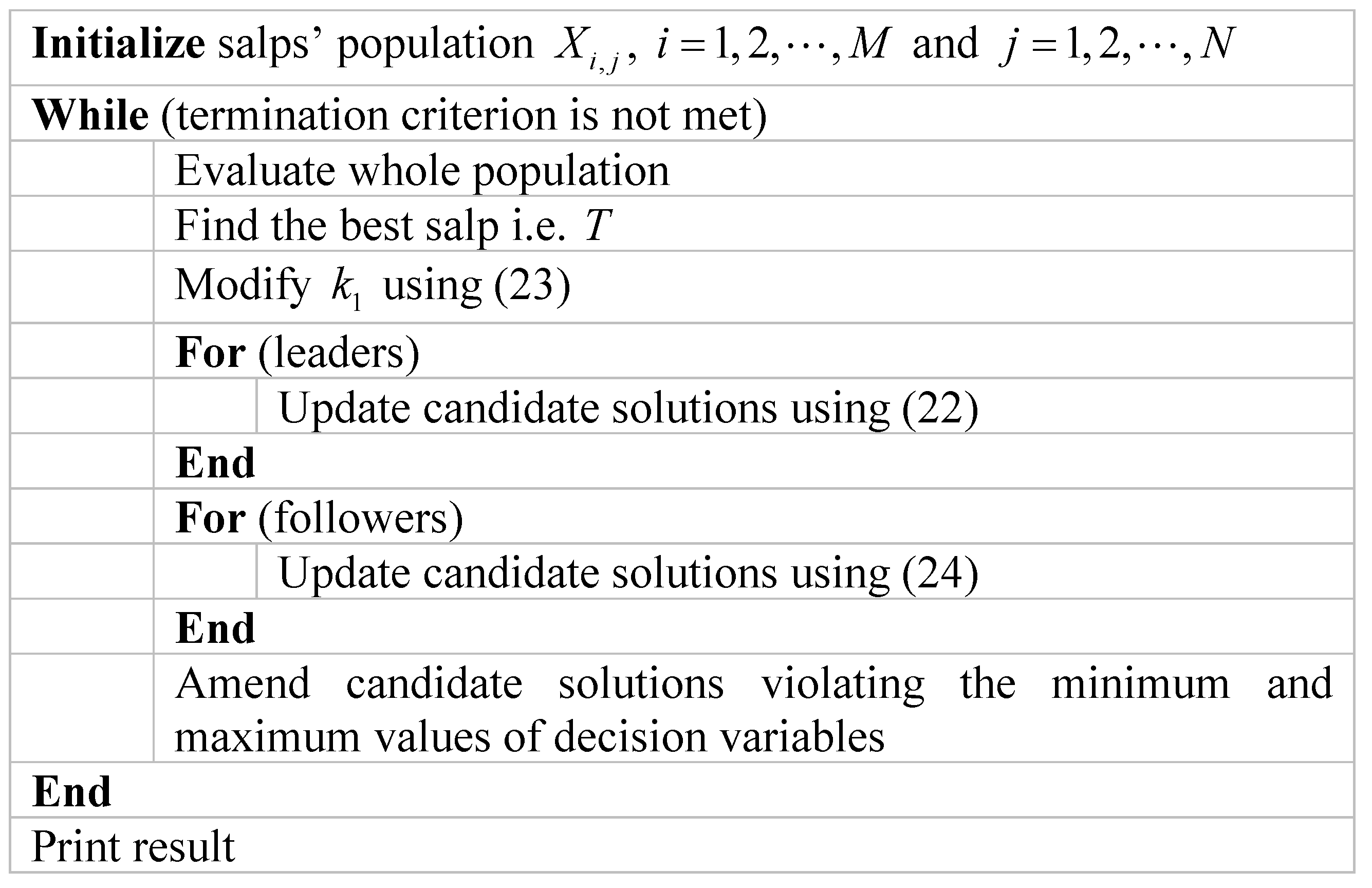
Salp swarm optimization (SSO) [25] is a nature inspired swarm-based meta-heuristic optimization algorithm. It is proposed recently by Mirjalili et al. [26] in 2017. This algorithm is derived from the swarming behavior of salps. Salps are found in deep ocean and are very similar to jelly fishes. The salps’ population can be categorized into (i) leaders and (ii) followers. The leaders lead the whole population while followers follow the instructions of leaders, directly or indirectly. The salps form chain to move. The salps at front of chain are known as leaders and remaining salps are known as followers. The better half of the population is treated as leader salps. However, remaining salps are considered as followers.

At first, the candidate solutions for leaders are updated. Since, followers follow the leaders, the candidate solutions for followers are updated using the solutions obtained for leaders. Suppose, $X_{i,j,}$ $i=1,2,\cdots ,M$ and $j=1,2,\cdots ,N$ denote initial candidate solutions for whole population where M and N represent population size and number of decision variables, respectively. The candidate solutions for leaders and followers are updated as follows.

4.1. Update of Candidate Solutions for Leaders

The candidate solutions for leaders are updated as

$$X_{i,j}^{new}=\left\{\begin{array}{cc}\hfill T_j+k_1((X_j^{+}-X_j^{-})k_2+X_j^{-})& \\ \hfill k_3\ge 0.5\\ \hfill T_j-k_1((X_j^{+}-X_j^{-})k_2+X_j^{-})\\ \hfill k_3<0.5\end{array}\right.$$

(22)

where $X_{i,j}^{new}$ is updated candidate solutions for $X_{i,j}$, $T_j$ is the position of food source, $X_j^{-}$ and $X_j^{+}$ represent the minimum and maximum values of decision variables, $k_2$ and $k_3$ are random numbers distributed uniformly in the range [0,1], and $k_1$ is modified during course of iterations as

$$k_1=2e^{-(\frac{4t}{T}{)}^2}$$

(23)

where T and t, respectively, are maximum number of iterations and current iteration.

4.2. Update of Candidate Solutions for Followers

The candidate solutions for followers are updated using the solutions of leaders. The mathematical expression used for updating the candidate solutions for followers is

$$X_{i,j}^{new}=\frac{X_{i,j}+X_{i-1,j}}{2}$$

(24)

where $X_{i,j}^{new}$ denotes updated candidate solution for follower $X_{i,j}$.

After updating the whole population as suggested in (22) and (24), candidate solutions violating the minimum and maximum values of decision variables are reinitialized at respective minimum and maximum values of decision variables. The pseudo code of SSO is presented in Figure 4.

4.3. Self-Learning Salp Swarm Optimization

A self-learning rule exploits the space in close proximity of the individual position to reach its global optimum [23]. The rule provides an opportunity to each learner to enhance the individual knowledge from self-surrounding space. This phase can be mathematically expressed as:

$$X_{i,j}^{new}\left(k\right)=X_{i,j}\left(k\right)(1+\lambda (r-0.5))$$

(25)

where, $X_{i,j}^{new}\left(k\right)$ is the new solution vector in this phase, $\lambda$ is the self-learning factor which determines the self-learning capability of each individual and $r\in [0,1]$. The value of $\lambda$ is considered 3 in this work. Update the solution vector, $X_{i,j}\left(k\right)$, using greedy selection. Thus, the updated $X_{i,j}\left(k\right)$ after this phase takes part in the next iteration.

5. Results and Comparisons

Two case studies are performed to highlight the findings and contributions of this article. One proportional-integral-derivative (PID) controller is designed for pressure-flux loop and other PID controller is tuned for pH-conductivity loop. In both the case studies, ISE of respective loop is minimized using SLSSO algorithm [23]. For fair presentation of efficacy of SLSSO algorithm, other algorithms namely, SSO, ABC, LJ, NMS, SCA and PSO are applied to tune the PID controller.

5.1. Case Study I

The results presented in this case study are obtained for pressure-flux loop by minimizing the performance index given in (19).

Table 4. Values of controller parameters for control loop I.

	ABC	LJ	NMS	PSO	SCA	SSO	SLSSO
$K_{p1}$	100	$95.21149$	$99.12550$	100	100	100	100
$K_{i1}$	100	100	$99.97304$	100	100	100	100
$K_{d1}$	$7.62050$	$27.67958$	$87.63271$	$11.42217$	$6.90757$	$7.71729$	$7.71729$
Mean	$2.07748$	$2.48291$	$2.23661$	$2.14169$	$2.24482$	$2.06634$	$2.06630$
min	$2.06630$	$2.08290$	$2.07079$	$2.06630$	$2.06630$	$2.06630$	$2.06630$
SD	$0.01233$	$0.22128$	$0.11820$	$0.17547$	$0.14121$	$0.00021$	$0.00002$

presents PID gains i.e., $K_p$, $K_i$, and $K_d$ obtained using SLSSO. Same table also tabulates the PID gains obtained using ABC, LJ, NMS, PSO, SCA and SSO. The mean and minimum values of ISE along with standard deviation are also presented in this table. The time domain specifications of step response obtained due to all algorithms (ABC, LJ, NMS, PSO, SCA, SSO and SLSSO) are tabulated in

Table 5. Comparisons of performance for control loop I.

	ABC	LJ	NMS	PSO	SCA	SSO	SLSSO
Rise time	13.07413	12.89226	12.75271	13.05996	13.07628	13.07377	13.07377
Settling time	23.48781	23.33940	23.51330	23.50330	23.56116	23.48848	23.48849

. The Figure 5 shows the step response obtained due to ABC, LJ, NMS, PSO, SCA, SSO and SLSSO. In addition to this, the response of pressure-flux loop for variable input due to SLSSO algorithm is plotted in Figure 6. The Figure 7 is showing the response with disturbance.

The mean value of ISE is minimum in case of SLSSO algorithm as shown in Table 4. The same is true for minimum value of ISE and standard deviation. The time domain specifications tabulated in Table 5 also supports the response obtained for pressure-flux loop. The step response of SLSSO algorithm is also reaching steady state as shown in Figure 5. For variable input and input having disturbance also, the SLSSO tuned controller is providing stable step response as shown in Figure 6 and Figure 7. Hence, it can be inferred that SLSSO algorithm is a better choice for tuning the PID gains for pressure-flux loop of DROP system.

5.2. Case Study II

This case study presents the analysis of results obtained for pH-conductivity loop. In this case, the performance index given in (20) is minimized using SLSSO algorithm. The PID gains ($K_p$, $K_i$, and $K_d$) obtained using SLSSO are presented in

Table 6. Values of controller parameters for control loop II.

	ABC	LJ	NMS	PSO	SCA	SSO	SLSSO
$K_{p2}$	−100	−79.93280	−99.29953	−100	−100	−100	−100
$K_{i2}$	−100	−85.25339	−84.53067	−100	−99.87994	−100	−100
$K_{d2}$	−100	−100	−98.73694	−100	−97.57030	−100	−100
Mean	$5.6866\times {10}^{-8}$	$1.7143\times {10}^{-7}$	$7.8758\times {10}^{-8}$	$6.2789\times {10}^{-8}$	$6.9226\times {10}^{-8}$	$5.2441\times {10}^{-8}$	$5.2396\times {10}^{-8}$
min	$5.2396\times {10}^{-8}$	$6.7616\times {10}^{-8}$	$5.5918\times {10}^{-8}$	$5.2396\times {10}^{-8}$	$5.3462\times {10}^{-8}$	$5.2396\times {10}^{-8}$	$5.2396\times {10}^{-8}$
SD	$2.3733\times {10}^{-8}$	$7.0918\times {10}^{-8}$	$2.3465\times {10}^{-8}$	$2.3200\times {10}^{-8}$	$1.8263\times {10}^{-8}$	$2.5872\times {10}^{-10}$	$2.6922\times {10}^{-23}$

. The Table 6 also provides gains obtained due to ABC, LJ, NMS, PSO, SCA and SSO. The mean and minimum values of ISE along with standard deviation are also shown in Table 6. The time domain specifications (rise time and settling time) of step response are given in

Table 7. Performance parameters using different algorithms for control loop II.

	ABC	LJ	NMS	PSO	SCA	SSO	SLSSO
Rise time	1.51527	1.84908	1.70050	1.51527	1.48409	1.51527	1.51527
Settling time	7.17368	8.61641	5.65413	7.17368	6.86024	7.17368	7.17368

which are obtained due to ABC, LJ, NMS, PSO, SCA, SSO and SLSSO. The Figure 8 plots the step response of pH-conductivity loop due to ABC, LJ, NMS, PSO, SCA, SSO and SLSSO. Moreover, the response of pH-conductivity loop for variable step input and step input having disturbance due to SLSSO algorithm is presented in Figure 9 and Figure 10, respectively.

In this case also, the mean value of ISE is the minimum for SLSSO algorithm as shown in Table 6. The same conclusion can be derived for minimum value of ISE and standard deviation. Table 6, Figure 8, Figure 9 and Figure 10 also prove that the SLSSO algorithm is an excellent alternative for tuning of PID controller for DROP system.

6. Conclusions

This contribution presented design of proportional-integral-derivative (PID) controller for Doha reverse osmosis plant (DROP). The DROP system is interacting in nature and has two inputs and two outputs resulting in TITO system. Since, this TITO system is interacting, the interaction effect should be eliminated before designing the PID controllers for two manipulated variables. In this article, simplified decoupling technique is adopted to design decoupler for interacting TITO DROP system. After designing the decopuler, two PID controllers for pressure flux and pH conductivity loops are designed to manipulate the pressure and pH in order to generate specified flux and conductivity. For designing the PID controllers, integral-square-error (ISE) of the respective loop is minimized using lelf-learning salp swarm optimization (SLSSO) algorithm [23]. It was proved that SLSSO algorithm is an excellent choice for tuning the PID gains for two loops of the DORP system.

As far as the further extension of this work is considered, it is aimed to obtain the interval model in discrete domain. The reduced-order model for discrete domain will be designed in further research. It would also be interesting to investigate the controller design using intelligent optimization algorithms like fireworks algorithm [12], bacterial foraging optimization [13], elephant herding optimization [10], whale optimization algorithm [2,14], monarch butterfly optimization [15], brain storm optimization [16], etc.

References

1. Rathore, N.S.; Singh, V.; Phuc, B.D.H. A modified controller design based on symbiotic organisms search optimization for desalination system. J. Water Supply Res. Technol. 2019, 68, 337–345. [Google Scholar] [CrossRef]
2. Rathore, N.S.; Singh, V. Whale optimisation algorithm-based controller design for reverse osmosis desalination plants. Int. J. Intell. Eng. Inform. 2019, 7, 77–88. [Google Scholar] [CrossRef]
3. Rathore, N.S.; Singh, V. Design of optimal PID controller for the reverse osmosis using teacher-learner-based-optimization. Membr. Water Treat. 2018, 9, 129–136. [Google Scholar]
4. Rathore, N.S.; Singh, V.; Kumar, B. Controller design for doha water treatment plant using grey wolf optimization. J. Intell. Fuzzy Syst. 2018, 35, 5329–5336. [Google Scholar] [CrossRef]
5. Alatiqi, I.; Ghabris, A.; Ebrahim, S. System identification and control of reverse osmosis desalination. Desalination 1989, 75, 119–140. [Google Scholar] [CrossRef]
6. Chaaben, A.B.; Andoulsi, R.; Sellami, A.; Mhiri, R. MIMO modeling approach for a small photovoltaic reverse osmosis desalination system. J. Appl. Fluid Mech. 2011, 4, 35–41. [Google Scholar]
7. Riverol, C.; Pilipovik, V. Mathematical modeling of perfect decoupled control system and its application: A reverse osmosis desalination industrial-scale unit. J. Anal. Methods Chem. 2005, 2005, 50–54. [Google Scholar] [CrossRef]
8. Rivas-Perez, R.; Sotomayor-Moriano, J.; Pérez-Zuñiga, G.; Soto-Angles, M.E. Real-time implementation of an expert model predictive controller in a pilot-scale reverse osmosis plant for brackish and seawater desalination. Appl. Sci. 2019, 9, 2932. [Google Scholar] [CrossRef] [Green Version]
9. Ho, W.K.; Gan, O.; Tay, E.B.; Ang, E. Performance and gain and phase margins of well-known PID tuning formulas. IEEE Trans. Control Syst. Technol. 1996, 4, 473–477. [Google Scholar] [CrossRef]
10. Gupta, S.; Singh, V.; Singh, S.; Prakash, T.; Rathore, N. Elephant herding optimization based PID controller tuning. Int. J. Adv. Technol. Eng. Explor. 2016, 3, 194. [Google Scholar] [CrossRef]
11. Rathore, N.; Chauhan, D.; Singh, V. Luus-Jaakola optimization procedure for PID controller tuning in reverse osmosis system. In Proceedings of the 23rd IRF International Conference, Chennai, India, 15 May 2016; pp. 12–15. [Google Scholar]
12. Gong, C. Opposition-based adaptive fireworks algorithm. Algorithms 2016, 9, 43. [Google Scholar] [CrossRef] [Green Version]
13. Lv, X.; Chen, H.; Zhang, Q.; Li, X.; Huang, H.; Wang, G. An improved bacterial-foraging optimization-based machine learning framework for predicting the severity of somatization disorder. Algorithms 2018, 11, 17. [Google Scholar] [CrossRef] [Green Version]
14. Prakash, T.; Singh, V.P.; Mohanty, S.R. A novel binary whale optimization algorithm-based optimal placement of phasor measurement units. In Handbook of Research on Power and Energy System Optimization; IGI Global: Hershey, PA, USA, 2018; pp. 115–138. [Google Scholar]
15. Chen, S.; Chen, R.; Gao, J. A monarch butterfly optimization for the dynamic vehicle routing problem. Algorithms 2017, 10, 107. [Google Scholar] [CrossRef] [Green Version]
16. Sato, M.; Fukuyama, Y.; Iizaka, T.; Matsui, T. Total optimization of energy networks in a smart city by multi-population global-best modified brain storm optimization with migration. Algorithms 2019, 12, 15. [Google Scholar] [CrossRef] [Green Version]
17. Rathore, N.S.; Kundariya, N.; Narain, A. PID controller tuning in reverse osmosis system based on particle swarm optimization. Int. J. Sci. Res. Publ. 2013, 3, 1–5. [Google Scholar]
18. Gambier, A.; Wellenreuther, A.; Badreddin, E. Control system design of reverse osmosis plants by using advanced optimization techniques. Desalin. Water Treat. 2009, 10, 200–209. [Google Scholar] [CrossRef] [Green Version]
19. Sobana, S.; Panda, R.C. Identification, modelling, and control of continuous reverse osmosis desalination system: A review. Sep. Sci. Technol. 2011, 46, 551–560. [Google Scholar] [CrossRef]
20. Azizipanah-Abarghooee, R.; Dehghanian, P.; Terzija, V. Practical multi-area bi-objective environmental economic dispatch equipped with a hybrid gradient search method and improved Jaya algorithm. IET Gener. Transm. Distrib. 2016, 10, 3580–3596. [Google Scholar] [CrossRef] [Green Version]
21. Singh, V.; Prakash, T.; Rathore, N.S.; Singh Chauhan, D.P.; Singh, S.P. Multilevel thresholding with membrane computing inspired TLBO. Int. J. Artif. Intell. Tools 2016, 25, 1650030. [Google Scholar] [CrossRef]
22. Singh, V.; Patnana, N.; Singh, S. PID controller tuning using hybrid optimisation technique based on Box’s evolutionary optimisation and teacher-learner-based-optimisation. Int. J. Comput. Aided Eng. Technol. 2020, 13, 258–270. [Google Scholar] [CrossRef]
23. Patnana, N.; Pattnaik, S.; Singh, V.P. Self-learning salp swarm optimization based controller design for photovoltaic reverse osmosis plant. Int. J. Model. Identif. Control 2020, 35, 10–23. [Google Scholar]
24. Liu, L.; Tian, S.; Xue, D.; Zhang, T.; Chen, Y.; Zhang, S. A review of industrial mimo decoupling control. Int. J. Control Autom. Syst. 2019, 17, 1246–1254. [Google Scholar] [CrossRef]
25. Patnana, N.; Pattnaik, S.; Singh, V.P. Salp swarm optimization based controller design for photovoltaic reverse osmosis plant. J. Inf. Optim. Sci. 2020, 41, 651–659. [Google Scholar] [CrossRef]
26. Mirjalili, S.; Gandomi, A.H.; Mirjalili, S.Z.; Saremi, S.; Faris, H.; Mirjalili, S.M. Salp Swarm Algorithm: A bio-inspired optimizer for engineering design problems. Adv. Eng. Softw. 2017, 114, 163–191. [Google Scholar] [CrossRef]
Figure 1. The block diagram of Doha reverse osmosis plant (DROP) system.
Algorithms 13 00287 g001
Figure 2. Block diagram.
Algorithms 13 00287 g002
Figure 3. Decoupler with TITO system.
Algorithms 13 00287 g003
Figure 4. Pseudo code of SSO algorithm.
Algorithms 13 00287 g004
Figure 5. Unit step response for control loop I.
Algorithms 13 00287 g005
Figure 6. Response of SLSSO-based controller for variable step input for loop I.
Algorithms 13 00287 g006
Figure 7. Response of SLSSO-based controller for variable step input with disturbance for loop I.
Algorithms 13 00287 g007
Figure 8. Unit step response for control loop II.
Algorithms 13 00287 g008
Figure 9. Response of SLSSO-based controller for variable step input for loop II.
Algorithms 13 00287 g009
Figure 10. Response of SLSSO-based controller for variable step input with disturbance for loop II.
Algorithms 13 00287 g010