A Feature-Weighted SVR Method Based on Kernel Space Feature

Abstract

Support Vector Regression (SVR), which converts the original low-dimensional problem to a high-dimensional kernel space linear problem by introducing kernel functions, has been successfully applied in system modeling. Regarding the classical SVR algorithm, the value of the features has been taken into account, while its contribution to the model output is omitted. Therefore, the construction of the kernel space may not be reasonable. In the paper, a Feature-Weighted SVR (FW-SVR) is presented. The range of the feature is matched with its contribution by properly assigning the weight of the input features in data pre-processing. FW-SVR optimizes the distribution of the sample points in the kernel space to make the minimizing of the structural risk more reasonable. Four synthetic datasets and seven real datasets are applied. A superior generalization ability is obtained by the proposed method.

1. Introduction

SVR is a powerful kernel-based method for regression problems [1,2,3]. It converts the original low-dimensional problem to a high-dimensional kernel space linear problem by introducing kernel functions. Regarding the system modeling with limited training samples, it balances the empirical risk and the confidence interval based on the principle of structural risk minimization. It avoids the over-fitting problem resulting from the overcomplex model and ensures the generalization performance of the model when it is sufficiently close to the training sample data [4,5,6,7,8]

The generalization ability of the SVR model is determined by the kernel space feature [9]. The value of kernel elements can be regarded as the similarity measure between samples in kernel space. The kernel function can simplify the calculation of the inner product in kernel space, and the curse of dimensionality is avoided. The contribution of the feature to the output is omitted in classical SVR. In some cases, such as when the dynamic range of an unimportant feature is large, the similarity of samples in kernel space may be dominated by the feature, so that the kernel matrix cannot deliver sufficient information about the training set to the model. Then, the optimization of structural risk minimization is affected.

At present, the research about SVR modeling focuses on the construction of the model and the optimization of the parameters [10,11,12,13], while the preprocessing of data is neglected. Data normalization methods, such as min-max normalization and Z-normalization, are the most widely-used preprocessing methods [14,15,16]. Min-max normalization converts raw data to [0, 1] or [−1, 1] by linearization. The Z-normalization method normalize the raw dataset to a dataset with a mean value of zero and a variance of one. The normalization method can overcome the numerical difficulties caused by the large difference of the dynamic range among input features. However, there is no evidence showing that normalization method will definitely improve the generalization performance. Whether to adopt the normalization is still based on the experience of engineers. In some literature, the feature selection is used to remove unimportant features from the training dataset and avoid the dominant influence of unimportant features on kernel space feature [17,18,19]. However, this will obviously lead to a lack of training information.

The weighted method is also used to improve the generalization ability. Zhang fan et al. developed a forecasting model using weighted SVR in which the weights were determined by the DE algorithm, and this model yielded high accuracy for building energy consumption forecasting [20]. Limei Liu combined weighted support vector regression machine with feature selection to predict electricity load, and the algorithm gave good prediction results [21]. Han, Xadditionally added weights to the slack variables in the constraints to predict house prices [22]. The above weighted SVR algorithms took the importance of sample points into account, and they can be used to minimize the influence of outliers or noises. However, the importance of the individual features is omitted. Recently, there have been some research works on feature weighting for the Support Vector Machine (SVM) classification problem [23,24,25,26,27]. Regretfully, it cannot be applied to the SVR because of the differences in the output.

The paper proposes an Feature-Weighted (FW)-SVR modeling method based on the kernel space feature. Firstly, we concluded that the classical methods are not reasonable by analyzing the similarity of sample points in the kernel space; because the value of the features has been taken into account, while the contribution to the model output is omitted. Then, we present the FW-SVR algorithm that makes the value of the features match their contribution by analyzing the limitation of the normalization algorithm and feature selection SVR algorithm.

The contribution of this work is two-fold. Firstly, the feature importance should be matched with the influence of the kernel space by analyzing the similarity of sample points in the kernel space. Secondly, a data pre-processing method of feature weighting based on the above conclusion is given. By adjusting the range of feature values by properly assigning the weight, the feature importance is matched with the influence of the kernel space, and the generalization ability of the model is improved. Then, the first conclusion is verified. The proposed method can be used to guide the data pre-processing of SVR modeling.

The paper is organized as follows: In Section 2 “Basic Review of SVR”, SVR theory is briefly described. In Section 3 “Feature-Weighted Support Vector Regression”, the necessity of the feature weighting is analyzed in theory, and then, the realization process of FW-SVR is introduced in detail. Simulation examples are given in Section 4 “Simulation Examples”. In Section 5 “Conclusions”, we come to a conclusion.

2. Basic Review of SVR

The training set is given as $T=\{(x_i,y_i),i=1,\cdots ,l\}$, where each $x_i\in R^n$ is the i-th input sample containing n features and $y_i\in R$ is the output sample. The model function determined by the SVR method can be regarded as a hyperplane in the kernel space. It is expressed as follows:

$$f\left(x\right)=<w,\varphi \left(x\right)>+b$$

(1)

where $\varphi \left(x\right)$ maps the raw data of input features to a high-dimensional kernel space, $w\in R^n$ is a weight vector of the hyperplane and b is a bias term.

An insensitive loss function $\epsilon >0$ is introduced to avoid over-fitting, and additional nonnegative slack variables ${\xi }_i,{\xi }_i^{\ast }$ are adopted to weaken the constraints of some certain sample points. SVR modeling is formulated as a convex quadratic programming problem expressed as follows:

$$\underset{w,\xi ,\xi \ast }{min}\frac{1}{2}{∥w∥}^2+C\sum _{i=1}^l\left({\xi }_i+{\xi }_i^{\ast }\right)$$

(2)

subject to:

$$\left\{\begin{array}{c}{y}_i-f\left(x_i\right)\le \epsilon +{\xi }_i\hfill \\ f\left(x_i\right)-y_i\le \epsilon +{\xi }_i^{\ast }\hfill \\ {\xi }_i,{\xi }_i^{\ast }\ge 0\hfill \end{array}\right.$$

(3)

where $C>0$ is a penalty parameter. The above convex quadratic programming problem can be solved by constructing a Lagrange function:

The above convex quadratic programming problem can be reformulated by constructing the Lagrange function:

$$\begin{array}{c}L=\frac{1}{2}{∥w∥}^2+C{\displaystyle \sum _{i=1}^l}\left({\xi }_i+{\xi }_i^{\ast }\right)-{\displaystyle \sum _{i=1}^l}\left({\xi }_i{\eta }_i+{\xi }_i^{\ast }{\eta }_i^{\ast }\right)-{\displaystyle \sum _{i=1}^l}{\alpha }_i\left[{\xi }_i+\epsilon +y_i-<w·\varphi \left(x_i\right)>-b\right]\hfill \\ -{\displaystyle \sum _{i=1}^l}{\alpha }_i^{\ast }\left[{\xi }_i+\epsilon -y_i+<w·\varphi \left(x_i\right)>+b\right]\hfill \end{array}$$

(4)

where ${\alpha }_i,{\alpha }_i^{\ast }\ge 0$ and ${\eta }_i,{\eta }_i^{\ast }\ge 0$ are Lagrange multipliers.

The kernel function $K\left(·,·\right)$, which satisfies the Mercer condition, is introduced to replace the inner product of the high dimensional kernel space in Equation (4). The commonly-used kernel functions are Gaussian kernel, linear kernel, sigmoid kernel, polynomial kernel, and so on [28,29,30]. These kernel functions are listed in

Table 1. Admissible kernel functions.

Name	Definition	Parameters
Gaussian kernel	$K\left(x_i,x\right)=\exp \left(-\gamma {∥x_i-x∥}^2\right)$	$\gamma$
Linear kernel	$K\left(x_i,x\right)=\left(x_i·x\right)$	-
Sigmoid kernel	$K\left(x_i,x\right)=\tanh \left(\gamma \left(x_i·x\right)+R\right)$	$\gamma$, R
Polynomial kernel	$K\left(x_i,x\right)={\left(\gamma \left(x_i·x\right)+R\right)}^d$	$\gamma$, R, d

.

The optimized problem can be expressed as follows:

$$\underset{\alpha ,\alpha \ast }{\mathrm{m}\mathrm{in}}\frac{1}{2}\sum _{i=1,j=1}^l\left({\alpha }_i-{\alpha }_i^{\ast }\right)\left({\alpha }_j-{\alpha }_j^{\ast }\right)K\left(x_i,x_j\right)+\epsilon \sum _{i=1}^l\left({\alpha }_i+{\alpha }_i^{\ast }\right)-\sum _{i=1}^l\left({\alpha }_i-{\alpha }_i^{\ast }\right)y_i$$

(5)

subject to:

$$\left\{\begin{array}{c}{\displaystyle \sum _{i=1}^l}\left({\alpha }_i-{\alpha }_i^{\ast }\right)=0\hfill \\ 0\le {\alpha }_i,{\alpha }_i^{\ast }\le C\hfill \end{array}\right.$$

(6)

The optimal solution can be obtained as follows:

$$\overline{\alpha }={\left({\overline{\alpha }}_1,{\overline{\alpha }}_1^{\ast },\dots ,{\overline{\alpha }}_l,{\overline{\alpha }}_l^{\ast }\right)}^{\mathrm{T}}$$

(7)

The model function Equation (1) can be further developed as follows:

$$f\left(x\right)=\sum _{i=1}^l\left({\overline{\alpha }}_i^{\ast }-{\overline{\alpha }}_i\right)K\left(x_i,x\right)+\overline{b}$$

(8)

3. Feature-Weighted Support Vector Regression

3.1. The Necessity of Feature Weighting

The similarity between sample points $x_i$ and $x_j$ in kernel space can be measured by calculating the distance $d_{ij}$ between $\varphi \left(x_i\right)$ and $\varphi \left(x_j\right)$.

$$\begin{array}{c}{d}_{ij}={∥\varphi \left(x_i\right)-\varphi \left(x_j\right)∥}^2\hfill \\ =〈\varphi \left(x_i\right)-\varphi \left(x_j\right),\varphi \left(x_i\right)-\varphi \left(x_j\right)〉\hfill \\ =〈\varphi \left(x_i\right),\varphi \left(x_i\right)〉-2〈\varphi \left(x_i\right),\varphi \left(x_j\right)〉+〈\varphi \left(x_j\right),\varphi \left(x_j\right)〉\hfill \\ =K\left(x_i,x_i\right)-2K\left(x_i,x_j\right)+K\left(x_j,x_j\right)\hfill \end{array}$$

(9)

When the Gauss kernel is adopted, $d_{ij}$ can be expressed as:

$$d_{ij}=2-2K\left(x_i,x_j\right)=2-2\exp \left(-\gamma {∥x_i-x_j∥}^2\right)$$

(10)

We can deduce that the greater similarity of the sample points, the smaller the distance between the mapping in the kernel space from Equation (10). When $x_i=x_j$, the most similarity is shown, and the distance $d_{ij}$ is zero.

A simple example is given to illustrate that the construction of the kernel space is not reasonable when the value of the feature is the only consideration and its contribution to the model output is neglected. There is a set of sample points $\left\{x_1,x_2,x_3\right\}$. Let $n=2$, $x_1,x_2,x_3\in R^n$, where $x_1=\left({\rho }_1+{\rho }_1^{\prime },{\rho }_2\right)$, $x_2=\left({\rho }_1,{\rho }_2+{\rho }_2^{\prime }\right)$, $x_3=\left({\rho }_1,{\rho }_2\right)$, ${\rho }_1,{\rho }_2\in R$, ${\rho }_1^{\prime },{\rho }_2^{\prime }\in R^{+}$; the first item of the sample point is Feature 1, and the second is Feature 2. Regarding $\varphi \left(x_1\right)$ and $\varphi \left(x_2\right)$, we can measure which one is more similar to $\varphi \left(x_3\right)$ by comparing the value of $d_{13}$ and $d_{23}$.

$$\left\{\begin{array}{c}{d}_{13}=2-2\exp \left(-\gamma {∥x_1-x_3∥}^2\right)=2-2\exp \left(-\gamma {{\rho }_1^{\prime }}^2\right)\hfill \\ d_{23}=2-2\exp \left(-\gamma {∥x_2-x_3∥}^2\right)=2-2\exp \left(-\gamma {{\rho }_2^{\prime }}^2\right)\hfill \end{array}\right.$$

(11)

The difference of the similarities of the two sample groups is decided by ${\rho }_1^{\prime }$ and ${\rho }_2^{\prime }$ accordingly. However, the contribution of the two features to the model output is quite different for the actual system in some situations. Assume that Feature 1 has a great contribution to the output and a small change of it can lead to a great change in the output. On the contrary, assume that the contribution of Feature 2 to the output is very small, and a large change can lead to a slight change in the output. When ${\rho }_1^{\prime }={\rho }_2^{\prime }$, it is obvious that the impact of the sample point $x_2$ on the output is more similar to that of $x_3$. When ${\rho }_1^{\prime }<{\rho }_2^{\prime }$, the influence of the sample point $x_2$ on the output may be more similar to that of $x_3$. The similarity to the contrary is deduced without considering the contribution of the features to the output. Therefore, the similarity of the sample points generated by the classical algorithm may be influenced greatly by the unimportant features with a large value range, resulting in the inconsistency of the similarities in the kernel space and in the actual situation.

We can deduce that the kernel element is used to simplify the computation of the inner product in the kernel space in solving the convex quadratic programming problems from Formulas (4)–(5). If the similarity cannot reflect the actual rule of the dataset and is dominated by unimportant features, the solution to the optimization problem by applying the structural risk minimization principle is unreasonable.

In the paper, the feature-weighting method is used to match the effect of the feature on the kernel space feature with its contribution to the model output. Regarding the k-th feature, if a weight value $w_k\in \left[0,1\right]$ is given, the kernel element will be changed as:

$$K_w(x_i,x_j)=\exp \left(-\gamma \left(\sum _{k=1}^n{\left(w_k\left(x_{ik}-x_{jk}\right)\right)}^2\right)\right)$$

(12)

Likewise, the weighted elements of the linear kernel can be rewritten as follows:

$$K_w\left(x_i,x_j\right)=\sum _{k=1}^n{w}_k^2{x}_{ik}{x}_{jk}$$

(13)

The weighted sigmoid kernel can be expressed as follows:

$$K_w\left(x_i,x_j\right)=\tanh \left(\gamma \sum _{k=1}^n{w}_k^2{x}_{ik}{x}_{jk}+R\right)$$

(14)

If the contribution of each feature to the output can be confirmed before model training and an appropriate weight value is assigned, the role played by the feature in the kernel space matches its contribution. When all the weights of the feature are one, the FW-SVR is degraded to the classical SVR. When the weight of a feature tends to be zero, it shows that the input feature has little influence on the output and means a dimension reduction. Moreover, the distance between the sample points is shortened, and the distribution of the samples is more compact.

3.2. The Implementation of the FW-SVR

The optimal combination of weights is the premise of realizing FW-SVR. In order to verify the conclusion of Section 3.1, we use the grid search method to get the optimal weight combination. Grid search is an exhaustive search method. Each feature has a set of weight values to select. All combinations are listed to generate the “grid”. Every combination is tested by SVR, and the optimal one is obtained.

The SVR training that introduces the weight value is shown as follows.

According to Equation (12), the convex quadratic programming problem of Formulas (5)–(6) can be rewritten as follows:

$$\underset{\alpha ,\alpha \ast }{\min }\frac{1}{2}\sum _{i=1,j=1}^l\left({\alpha }_i-{\alpha }_i^{\ast }\right)\left({\alpha }_j-{\alpha }_j^{\ast }\right)K_w\left(x_i,x_j\right)+\epsilon \sum _{i=1}^l\left({\alpha }_i+{\alpha }_i^{\ast }\right)-\sum _{i=1}^l\left({\alpha }_i-{\alpha }_i^{\ast }\right)y_i$$

(15)

subject to:

$$\left\{\begin{array}{c}{\displaystyle \sum _{i=1}^l}\left({\alpha }_i-{\alpha }_i^{\ast }\right)=0\hfill \\ 0\le {\alpha }_i,{\alpha }_i^{\ast }\le C\hfill \end{array}\right.$$

(16)

The optimal solution can be obtained as $\overline{\alpha }={\left({\overline{\alpha }}_1,{\overline{\alpha }}_1^{\ast },\dots ,{\overline{\alpha }}_l,{\overline{\alpha }}_l^{\ast }\right)}^{\mathrm{T}}$.

The model function of FW-SVR can be expressed as follows:

$$f\left(x\right)=\sum _{i=1}^l\left({\overline{\alpha }}_i^{\ast }-{\overline{\alpha }}_i\right)K_w\left(x_i,x\right)+\overline{b}$$

(17)

4. Simulation Examples

In this Section, four synthetic datasets and seven real datasets are employed to verify the feasibility of the FW-SVR. All the simulations are implemented on a Windows 10 PC with Intel Core i5-3740 CPU (3.2 GHz) and 4.0 GB RAM by MATLAB R2013a. The SVR training and the test algorithm are implemented in LIBSVM 3.22 [31]. The parameters for each approach on each dataset are optimized by using grid search with five-fold cross-validation on a sample of the training set [32,33].

The Root Mean Square Error (RMSE) is employed to evaluate the feasibility of the FW-SVR method.

$$\mathrm{RMSE}=\sqrt{\frac{1}{l}\sum _{i=1}^l{\left[y_i-f\left(x_i\right)\right]}^2}$$

(18)

where $y_i$ is the actual output sample and $f\left(x_i\right)$ is its corresponding predicted value. The smaller the value of RMSE, the better its generalization ability.

Synthetic Datasets

The definitions of these functions are listed in

Table 2. Functions used to generate synthetic datasets.

Name	Function Definition	Domain of Definition
F1	$y_i=\frac{\sin \left(x_{i1}\right)}{x_{i1}}+\frac{x_{i2}}{1000}+\sigma$	$x_{i1}\in [-10,10],x_{i2}\in [-30,30]$
F2	$y_i=10\cos \left(3x_{i1}\right)+\frac{1}{10}\sin \left(x_{i2}\right)+\sigma$	$x_{i1},x_{i2}\in [-2\pi ,2\pi ]$
F3	$y_i={x_{i1}}^2\sin \left(x_{i2}\right)+\frac{3}{1+e^{-x_{i3}}}+\sigma$	$x_{i1}\in [-3,3],x_{i2}\in [-2\pi ,2\pi ],x_{i3}\in [-200,200]$
F4	$y_i=\frac{x_{i1}}{100}+\frac{x_{i2}}{10000}+\sigma$	$x_{i1}\in [-10,10],x_{i2}\in [-30,30]$

.

Where, $\sigma$ is the added Gaussian noise with a mean of zero and a standard deviation of 0.01.

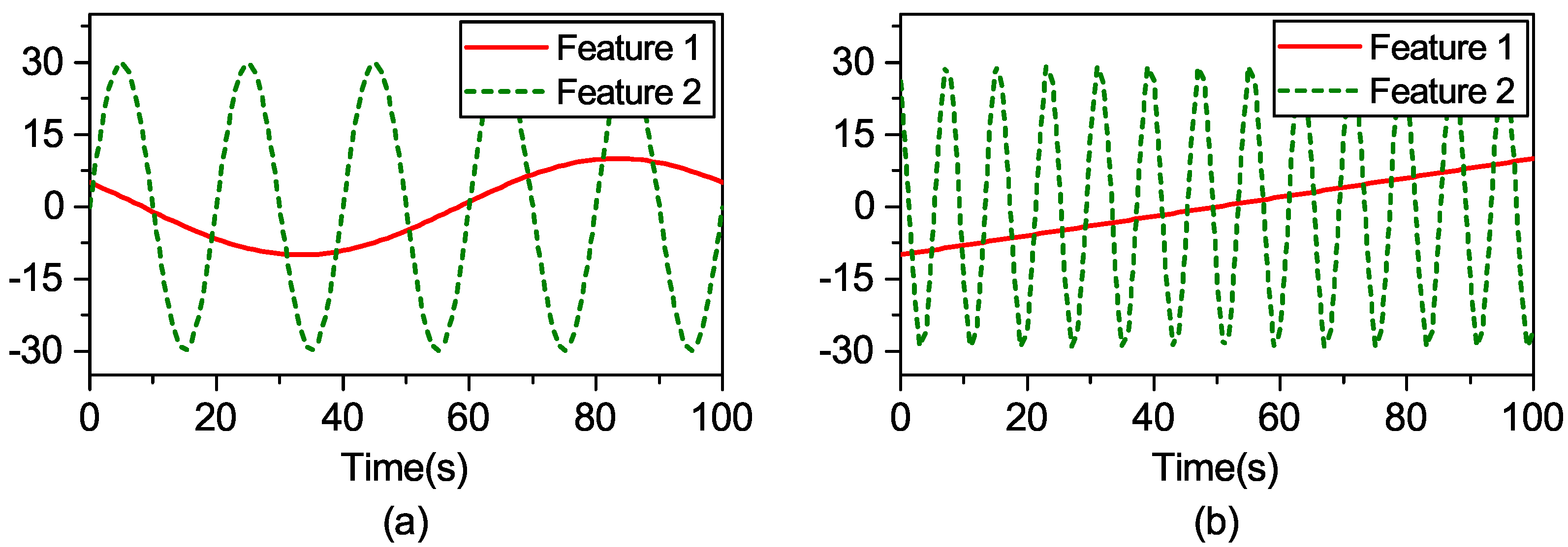
The synthetic dataset “F1” is chosen as an example. Feature 1 ($x_{i1}$) and Feature 2 ($x_{i2}$) in the training data are taken from the sinusoidal signals of 0.01 Hz and 0.05 Hz, respectively. Their corresponding test data are extracted from linear functions and the sinusoidal signal 0.125 Hz, respectively, as shown in Figure 1.

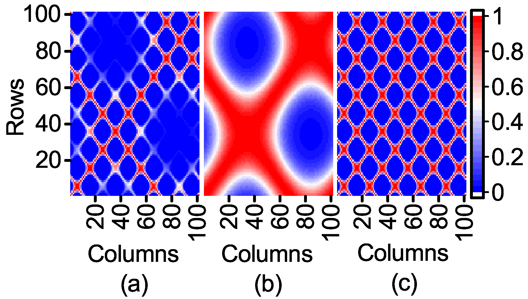
The expression of F1 shows that the range of the first item affected by Feature 1 is [−0.2172, 1] and that of the second item affected by Feature 2 is restricted to [−0.03, 0.03]. It is deduced that Feature 1, which has a great contribution to the output, is an important feature, while Feature 2 is to the contrary. However, the contribution of Feature 2 to the output of the model is neglected when the kernel matrix is calculated. In order to observe the influence of Feature 1 and Feature 2 on the kernel matrix, a kernel width $\gamma$ = 0.01 is used to compare the three kernel matrices visualized in 2D heat-maps as follows.

According to Equation (12), the kernel matrix can fully reflect the similarity between the sample points in kernel space. The similarity of the sample points in Figure 2c is clearly shown in Figure 2a, while the influence of Feature 1 with a high contribution to the output is obviously weakened.

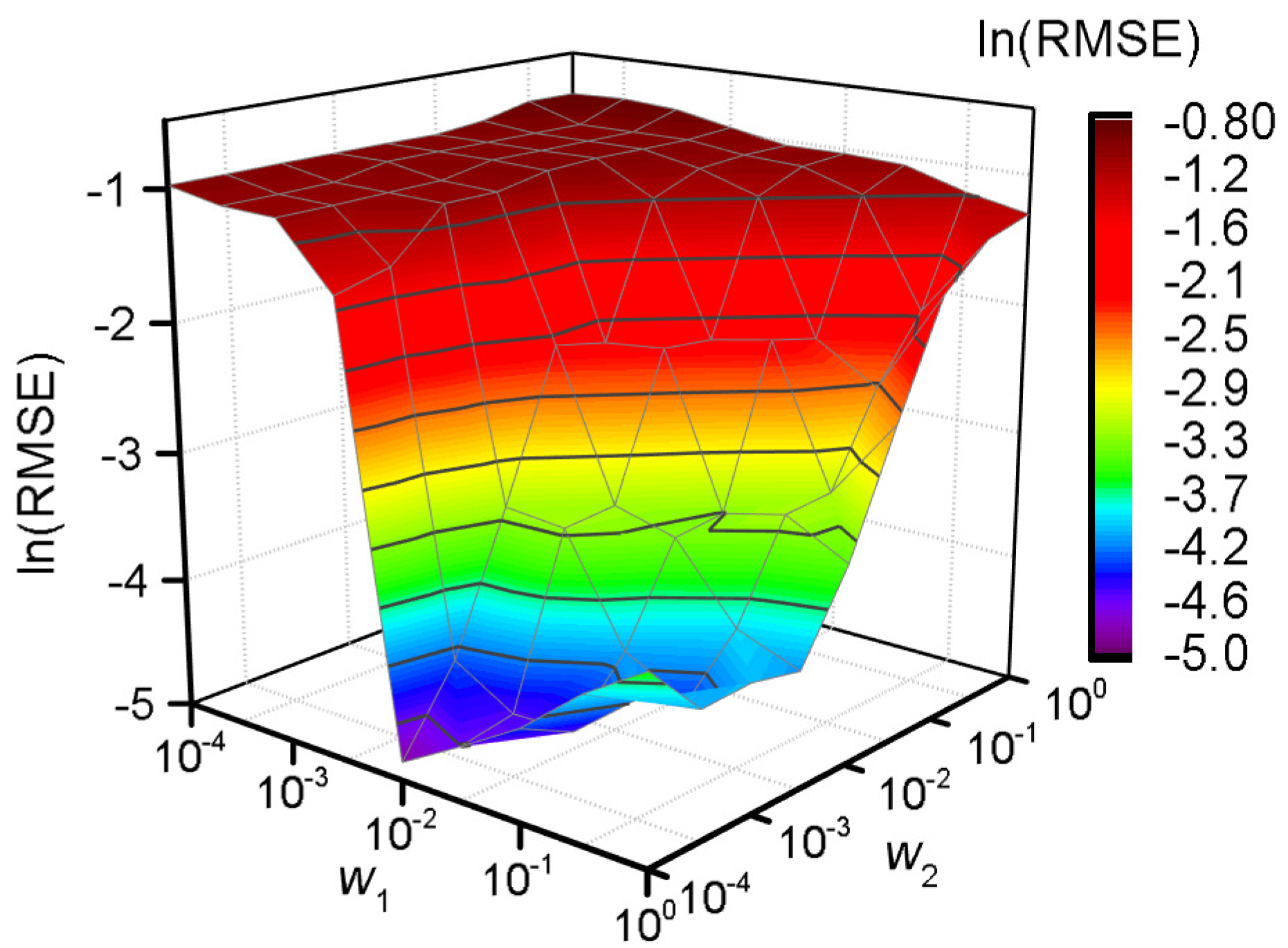
A grid search method is applied to obtain the corresponding RMSE for each possible combination of $w_1,w_2$ to verify the necessity of feature weighting [34]. The value of $w_1$ and $w_2$ is searched from the set $\left\{{10}^{-4},{10}^{-3.5},{10}^{-3},\cdots ,{10}^0\right\}$. The model performance is shown as Figure 3 accordingly.

According to Figure 3, a better generalization ability occurs when the value of $w_1/w_2$ is around 100, and the best is acquired when $w_1={10}^{-2}$ and $w_2={10}^{-4}$. As a whole, a better generalization ability can be obtained when $w_1>w_2$ vs. when $w_1<w_2$. The FW-SVR is degraded to the classical SVR when $w_1=w_2=1$, and the generalization ability of the model is poor.

We compare the feature weighting method with the feature selection and the normalization. In feature weighting, $w_1={10}^{-2}$ and $w_2={10}^{-4}$. In feature selection, Feature 2 is deleted. In the normalization method, the min-max normalization and the Z-normalization are employed.

Min-max normalization converts raw data to [0, 1] by linearization. The k-th feature of the i-th sample $x_{ik}$ is normalized to $x_{ik}^{\prime }$:

$$x_{ik}^{\prime }=\frac{x_{ik}-{x_k}_{min}}{{x_k}_{max}-{x_k}_{min}}$$

(19)

where ${x_k}_{max},{x_k}_{min}$ is the maximum and minimum value of the k-th feature, respectively.

The Z-normalization method normalizes the raw data to a dataset with a mean value of zero and a variance of one.

$$x_{ik}^{\prime }=\frac{x_{ik}-{\mu }_k}{{\sigma }_k}$$

(20)

where ${\mu }_k,{\sigma }_k$ is the mean and standard deviation of the k-th feature, respectively.

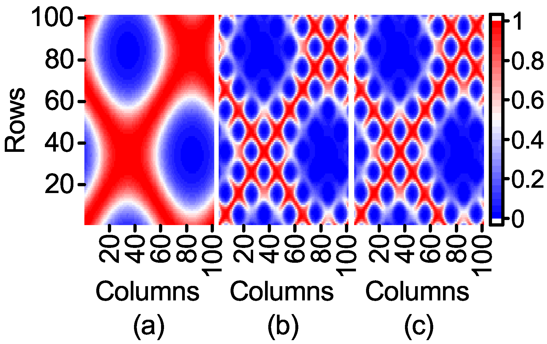
Firstly, the kernel matrix generated by feature weighting and by other methods is compared. In order to facilitate the comparison, when the parameter $\gamma$ is selected, the result consistency of Feature 1 is calculated as the standard of nuclear element calculation, because weighting and normalization will change the value of the feature. The kernel matrix generated by the above method is shown in Figure 4.

As can be seen from Figure 4, the feature weighting reduces the influence of Feature 2 on the kernel matrix. Figure 4a is similar to Figure 2b. However, the feature weighting preserves the information of Feature 2 compared to the feature selection. It can be deduced from Figure 4b,c that the normalization method can weaken the influence of Feature 2. However, its influence is still great. As the range of Feature 1 and Feature 2 is essentially the same in normalization, the contributions of Feature 1 and Feature 2 are much the same. When the range of unimportant features is greatly wider than that of important features, the normalization method can largely reduce the influence of unimportant features. On the contrary, the normalization method will increase their influence.

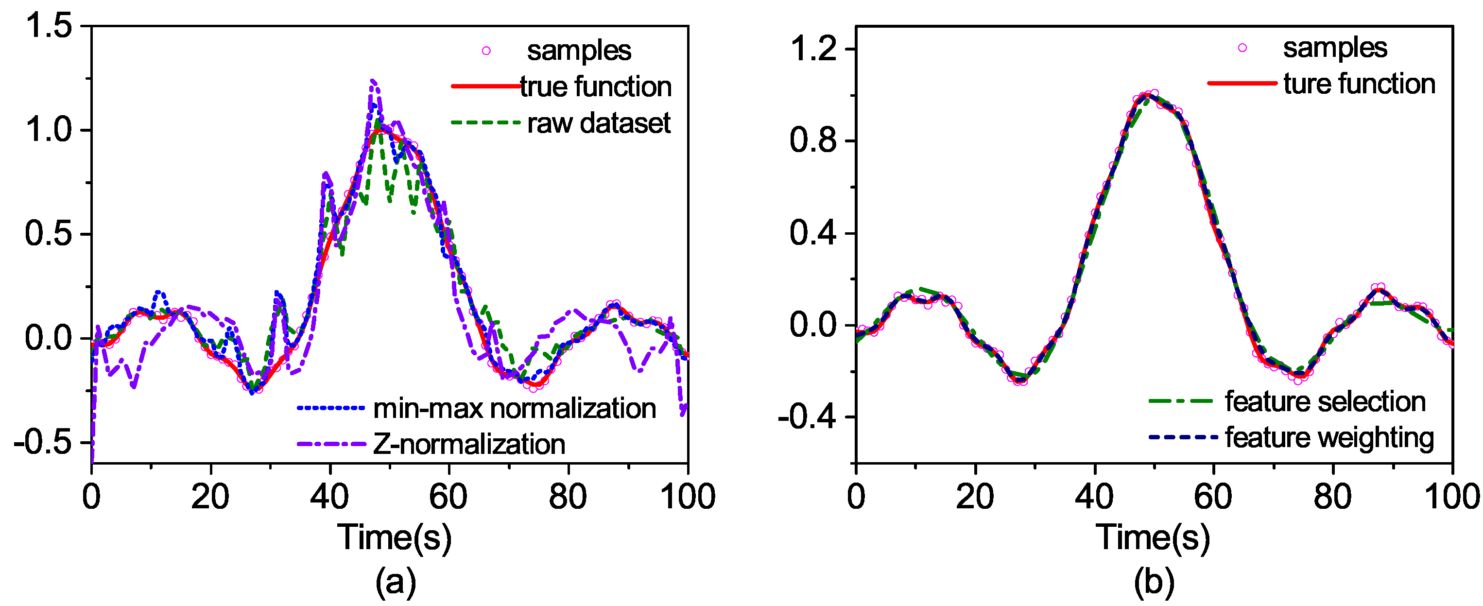
Then, the feature weighting is compared with the raw dataset, the feature selection and the normalization to observe the differences in the generalization ability. The search range of parameters C and $\gamma$ is $\left[2^{-8},2^9\right]$ and $\left[2^{-8},2^{10}\right]$, respectively, and $\epsilon$ is set to 0.0064. The optimal hyper-parameter is obtained by five-fold cross-validation. The prediction outputs for the test set are shown in Figure 5.

As can be seen from Figure 5, the prediction curve with raw data is quite different from the real output and the two prediction curves with normalized data, as well. The feature selection achieves better results. However, under-fitting occurs because of the deletion of Feature 2. The best prediction result is derived from the feature weighting method.

We model the synthetic datasets in Table 2 to compare the above methods. For the feature selection, all possible feature combinations are tested in order to get the optimal one. It is used to be compared with the feature weighting. The program is repeated 10 times. The optimal combination of weights is shown in

Table 3. The optimal combination of weights for the synthetic datasets.

Function Name	The Optimal Combination of Weights $\left\{{\mathit{w}}_1,{\mathit{w}}_2,\cdots ,{\mathit{w}}_{\mathit{n}}\right\}$
F1	$\left\{{10}^{-2},{10}^{-4}\right\}$
F2	$\left\{{10}^0,{10}^{-3}\right\}$
F3	$\left\{{10}^0,{10}^0,{10}^{-2}\right\}$
F4	$\left\{{10}^{-3},{10}^{-4}\right\}$

, and the results are shown in

Table 4. Performance comparison of SVR modeling for the synthetic datasets.

Function Name	Kernel Type	Feature Weighting	Raw Data	Feature Selection	Min-Max Normalization	Z-Normalization
F1	Gaussian	0.0095 ± 0.0030	0.1067 ± 0.0065	0.0299 ± 0.0008	0.1006 ± 0.0195	0.1483 ± 0.0090
	linear	0.3799 ± 0.0034	0.3765 ± 0.0052	0.3810 ± 0.0034	0.3786 ± 0.0011	0.3788 ± 0.0010
	sigmoid	0.4164 ± 0.0481	0.3826 ± 0.0012	0.4597 ± 0.0499	0.3820 ± 0.0045	0.4062 ± 0.0072
F2	Gaussian	0.0864 ± 0.0024	5.9620 ± 0.0005	0.0897 ± 0.0013	5.9021 ± 0.0004	8.0087 ± 0.0008
	linear	7.3255 ± 0.0010	7.3365 ± 0.0011	7.5173 ± 0.0025	7.3257 ± 0.0008	7.3392 ± 0.0011
	sigmoid	7.3919 ± 0.0021	8.0011 ± 0.0029	7.3673 ± 0.0020	7.5199 ± 0.0151	8.0690 ± 0.0786
F3	Gaussian	1.3450 ± 0.0095	3.1562 ± 0.0100	2.3098 ± 0.0050	2.9849 ± 0.0066	2.7477 ± 0.0070
	linear	2.7559 ± 0.0009	2.7533 ± 0.0030	3.1054 ± 0.0020	3.1169 ± 0.0026	3.0984 ± 0.0022
	sigmoid	2.8319 ± 0.0525	2.6547 ± 0.0138	3.2840 ± 0.0011	3.1158 ± 0.0188	3.0931 ± 0.0020
F4	Gaussian	0.0037 ± 0.0009	0.0076 ± 0.0007	0.0293 ± 0.0015	0.0219 ± 0.0031	0.2133 ± 0.0035
	linear	0.0120 ± 0.0034	0.0744 ± 0.0485	0.0214 ± 0.0002	0.0021 ± 0.0008	0.2437 ± 0.0010
	sigmoid	0.0024 ± 0.0005	1.2928 ± 0.0122	0.0232 ± 0.0005	0.0116 ± 0.0011	0.2340 ± 0.0026

, in which bold values indicate the method with the best performance.

Finally, we randomly chose seven UCIbenchmark datasets [35]. The grid search method is used to select the optimal combination of weights from the set $\left\{{10}^{-4},{10}^{-3},{10}^{-2},{10}^{-1},{10}^0\right\}$. The optimal combination of weights is shown in

Table 5. The optimal combination of weights for the UCIdatasets.

Datasets (Training Size, Test Size)	The Optimal Combination of Weights $\left\{{\mathit{w}}_1,{\mathit{w}}_2,\cdots ,{\mathit{w}}_{\mathit{n}}\right\}$
CCPP(300 × 4, 9268 × 4)	$\left\{{10}^{-1},{10}^{-1},{10}^{-2},{10}^{-1}\right\}$
Airfoil (376 × 5, 1127 × 5)	$\left\{{10}^{-4},{10}^{-2},{10}^0,{10}^{-3},{10}^0\right\}$
Servo (84 × 4, 83 × 4)	$\left\{{10}^0,{10}^{-1},{10}^{-1},{10}^0\right\}$
Yacht (154 × 6, 154 × 6)	$\left\{{10}^{-2},{10}^{-1},{10}^{-4},{10}^{-2},{10}^{-2},{10}^0\right\}$
Auto-MPG (196 × 7, 196 × 7)	$\left\{{10}^{-4},{10}^{-4},{10}^{-2},{10}^{-4},{10}^{-1},{10}^{-1},{10}^{-2}\right\}$
Machine CPU (109×7, 100×7)	$\left\{{10}^{-3},{10}^{-4},{10}^{-4},{10}^{-2},{10}^{-1},{10}^{-4},{10}^{-2}\right\}$
Concrete (300 × 8, 730 × 8)	$\left\{{10}^{-3},{10}^{-3},{10}^{-4},{10}^{-2},{10}^{-1},{10}^{-4},{10}^{-4},{10}^{-1}\right\}$

, and the results are compared as in

Table 6. Performance comparison of SVR modeling for the UCI datasets.

Function Name	Kernel Type	Feature Weighting	Raw Data	Feature Selection	Min-Max Normalization	Z-Normalization
CCPP	Gaussian	4.3739	5.9063	4.7865	4.4532	4.4225
	linear	4.6558	5.7354	5.0788	4.6372	4.6559
	sigmoid	17.3939	17.3939	17.3939	4.6706	4.6641
Airfoil	Gaussian	2.6293	6.2425	6.2426	3.0588	3.0773
	linear	5.0954	9.3584	6.2426	4.9028	4.9029
	sigmoid	5.2459	6.8646	6.7541	4.7974	4.9155
Servo	Gaussian	1.0071	1.1454	1.2059	1.2255	1.2411
	linear	1.2451	1.2457	1.3233	1.2455	1.2457
	sigmoid	1.5365	1.3881	1.3658	1.2510	1.2147
Yacht	Gaussian	0.8789	20.9455	2.0736	15.0084	15.6554
	linear	11.5317	12.0055	12.0191	11.5062	11.5056
	sigmoid	11.6018	17.1246	16.9336	11.6398	12.3480
Auto-MPG	Gaussian	2.5555	7.0208	3.1720	2.9386	3.0382
	linear	3.3510	3.3589	3.7220	3.4881	3.4849
	sigmoid	6.1315	7.8074	7.8074	3.5747	3.6064
Machine CPU	Gaussian	20.9777	158.0651	57.1354	48.7881	65.9913
	linear	56.2433	71.8240	86.0324	61.8386	59.7331
	sigmoid	97.8911	172.4349	172.4349	78.8043	84.4713
Concrete	Gaussian	8.2697	18.0116	15.5832	11.3164	11.7239
	linear	13.0202	17.1842	16.1212	10.3878	11.3107
	sigmoid	13.0202	17.1842	17.1666	10.3878	11.3107

, in which bold values indicate the method with the best performance.

The Wilcoxon signed rank tests [36] at the 0.05 significance level are implemented to test the differences between the feature weighting and other data pre-processing techniques to substantiate the indications in Table 4 and Table 6. The test results are presented in

Table 7. Wilcoxon signed rank test for the prediction results.

Kernel Type	Raw Data	Feature Selection	Min-Max Normalization	Z-Normalization
Gaussian	9.7656 ×${10}^{-4}$	9.7656 ×${10}^{-4}$	9.7656 ×${10}^{-4}$	9.7656 ×${10}^{-4}$
Linear	0.0117	0.0039	1.0000	0.4961
Sigmoid	0.0391	0.0234	0.0547	0.0977

Cell: p value.

. The prediction results on F1 and F2 using linear and sigmoid kernels were both unacceptable and were not included in this test.

According to Table 4 and Table 6, FW-SVR achieves a competitive generalization performance with both synthetic datasets and real datasets. The FW-SVR that uses the Gaussian kernel performs reasonably well on all 11 datasets. Note that the results on F1 and F2 are both unacceptable because of under-fitting for the linear kernel and the sigmoid kernel. The two datasets are not included in the following comparison. As for the linear kernel, three optimal results and three suboptimal results are obtained by FW-SVR. In addition, there are three results that are close to the optimal ones. As for the sigmoid kernel, FW-SVR achieves a competitive generalization performance on synthetic datasets. For example, the mean RMSE o 0.0024 on F4 is better than the value of 0.0120 of the Gaussian kernel. However, FW-SVR is not the optimal choice for the UCI datasets, as shown in Table 6. In general, the overall results obtained by the Wilcoxon tests presented in Table 7 show that the FW-SVR achieves the best generalization performance in comparison with the other five data pre-processing methods when the most suitable kernel type is selected. Comparing the five methods, we deduce that the contribution of the feature to the output is taken into account by FW-SVR, which reduces the influence of unimportant features on the kernel space feature.

5. Conclusions

In the paper, we propose an FW-SVR that matches the effect of the feature on the kernel space feature with its contribution to the model output. Analyzing the similarity of sample points in kernel space, we concluded that the FW-SVR makes the distribution of the sample points in kernel space more reasonable and is important to increase the generalization ability. Numerical experiments show the effectiveness of the proposed algorithm. Our future work will focus on automatic identification of the contribution to assign an optimal weight combination.

References

1. Vapnik, V.N. An overview of statistical learning theory. IEEE Trans. Neural Netw. 1999, 10, 988–999. [Google Scholar] [CrossRef] [PubMed]
2. Smola, A.J.; Schölkopf, B. A tutorial on support vector regression. Stat. Comput. 2004, 14, 199–222. [Google Scholar] [CrossRef]
3. Wang, D.; Lin, H. A new class of dual support vector machine NPID controller used for predictive control. IEEJ Trans. Electr. Electron. Eng. 2015, 10, 453–457. [Google Scholar] [CrossRef]
4. Paliwal, M.; Kumar, U.A. Neural networks and statistical techniques: A review of applications. Expert Syst. Appl. 2009, 36, 2–17. [Google Scholar] [CrossRef]
5. Sapankevych, N.I.; Sankar, R. Time series prediction using support vector machines: a survey. IEEE Comput. Intell. Mag. 2009, 4, 24–38. [Google Scholar] [CrossRef]
6. Tanveer, M.; Mangal, M.; Ahmad, I.; Shao, Y.H. One norm linear programming support vector regression. Neurocomputing 2016, 173, 1508–1518. [Google Scholar] [CrossRef]
7. Nekoei, M.; Mohammadhosseini, M.; Pourbasheer, E. QSAR study of VEGFR-2 inhibitors by using genetic algorithm-multiple linear regressions (GA-MLR) and genetic algorithm-support vector machine (GA-SVM): A comparative approach. Med. Chem. Res. 2015, 24, 3037–3046. [Google Scholar] [CrossRef]
8. Fujita, K.; Deng, M.; Wakimoto, S. A Miniature Pneumatic Bending Rubber Actuator Controlled by Using the PSO-SVR-Based Motion Estimation Method with the Generalized Gaussian Kernel. Actuators. 2017, 6, 6. [Google Scholar] [CrossRef]
9. Xie, M.; Wang, D.; Xie, L. One SVR modeling method based on kernel space feature. IEEJ Trans. Electr. Electron. Eng. 2018, 13, 168–174. [Google Scholar] [CrossRef]
10. Zhang, X.; Qiu, D.; Chen, F. Support vector machine with parameter optimization by a novel hybrid method and its application to fault diagnosis. Neurocomputing 2015, 149, 641–651. [Google Scholar] [CrossRef]
11. Tian, M.; Wang, W. An efficient Gaussian kernel optimization based on centered kernel polarization criterion. Inf. Sci. 2015, 322, 133–149. [Google Scholar] [CrossRef]
12. Fu, Y.; Wang, S. A No Reference Image Quality Assessment Metric Based on Visual Perception. Algorithms 2016, 9, 87. [Google Scholar] [CrossRef]
13. Meighani, H.M.; Ghotbi, C.; Behbahani, T.J.; Sharifi, K. Evaluation of PC-SAFT model and Support Vector Regression (SVR) approach in prediction of asphaltene precipitation using the titration data. Fluid Phase Equilib. 2018, 456, 171–183. [Google Scholar] [CrossRef]
14. Dunn, J.C. A Fuzzy Relative of the ISODATA Process and Its Use in Detecting Compact Well-Separated Clusters. Cybern. Syst. 1973, 3, 32–57. [Google Scholar] [CrossRef]
15. Lu, C.J. Hybridizing nonlinear independent component analysis and support vector regression with particle swarm optimization for stock index forecasting. Neural Comput. Appl. 2013, 23, 2417–2427. [Google Scholar] [CrossRef]
16. Yalavarthi, R.; Shashi, M. Atmospheric Temperature Prediction using Support Vector Machines. Int. J. Comput. Theory Eng. 2009, 1, 55–58. [Google Scholar]
17. Miao, F.; Fu, N.; Zhang, Y.T.; Ding, X.R.; Hong, X.; He, Q.; Li, Y. A Novel Continuous Blood Pressure Estimation Approach Based on Data Mining Techniques. IEEE J. Biomed. Health Inform. 2017, 21, 1730–1740. [Google Scholar] [CrossRef] [PubMed]
18. Papari, B.; Edrington, C.S.; Kavousi-Fard, F. An Effective Fuzzy Feature Selection and Prediction Method for Modeling Tidal Current: A Case of Persian Gulf. IEEE Trans. Geosci. Remote Sens. 2017, 55, 4956–4961. [Google Scholar] [CrossRef]
19. Taghizadeh-Mehrjardi, R.; Neupane, R.; Sood, K.; Kumar, S. Artificial bee colony feature selection algorithm combined with machine learning algorithms to predict vertical and lateral distribution of soil organic matter in South Dakota, USA. Carbon Manag. 2017, 8, 277–291. [Google Scholar] [CrossRef]
20. Zhang, F.; Deb, C.; Lee, S.E.; Yang, J.; Shah, K.W. Time series forecasting for building energy consumption using weighted Support Vector Regression with differential evolution optimization technique. Energy Build. 2016, 126, 94–103. [Google Scholar] [CrossRef]
21. Liu, L. Short-term load forecasting based on correlation coefficient and weighted support vector regression machine. In Proceedings of the 2015 4th International Conference on Information Technology and Management Innovation (ICITMI 2015), Shenzhen, China, 12–13 September 2015. [Google Scholar]
22. Han, X.; Clemmensen, L. On Weighted Support Vector Regression. Qual. Reliab. Eng. Int. 2014, 30, 891–903. [Google Scholar] [CrossRef]
23. Preetha, R.; Bhanumathi, R.; Suresh, G.R. Immune Feature Weighted Least-Squares Support Vector Machine for Brain Tumor Detection Using MR Images. IETE J. Res. 2016, 62, 873–884. [Google Scholar] [CrossRef]
24. Qi, B.; Zhao, C.; Yin, G. Feature weighting algorithms for classification of hyperspectral images using a support vector machine. Appl. Opt. 2014, 53, 2839–2846. [Google Scholar] [CrossRef] [PubMed]
25. Shi, J.; Zhang, S.; Qiu, L. Credit scoring by feature-weighted support vector machines. J. Zhejiang Univ. Sci. C Comput. Electron. 2013, 14, 197–204. [Google Scholar] [CrossRef]
26. Deng, W.; Zhou, J. Approach for feature weighted support vector machine and its application in flood disaster evaluation. Disaster Adv. 2013, 6, 51–58. [Google Scholar]
27. Guo, L.; Zhao, L.; Wu, Y.; Li, Y.; Xu, G.; Yan, Q. Tumor Detection in MR Images Using One-Class Immune Feature Weighted SVMs. IEEE Trans. Magn. 2011, 47, 3849–3852. [Google Scholar] [CrossRef]
28. Babaud, J.; Witkin, A.P.; Baudin, M.; Duda, R.O. Uniqueness of the Gaussian Kernel for Scale-Space Filtering. IEEE Trans. Pattern Anal. Mach. Intell. 1986, PAMI-8, 26–33. [Google Scholar] [CrossRef]
29. Keerthi, S.S.; Lin, C.J. Asymptotic Behaviors of Support Vector Machines with Gaussian Kernel. Neural Comput. 2003, 15, 1667–1689. [Google Scholar] [CrossRef] [PubMed]
30. Howley, T.; Madden, M.G. The Genetic Kernel Support Vector Machine: Description and Evaluation. Artif. Intell. Rev. 2005, 24, 379–395. [Google Scholar] [CrossRef]
31. Chang, C.C.; Lin, C.J. LIBSVM: A library for support vector machines. ACM Trans. Intell. Syst. Technol. (TIST) 2011, 2, 1–27. [Google Scholar] [CrossRef]
32. Zhang, P. Model Selection Via Multifold Cross Validation. Ann. Stat. 1993, 21, 299–313. [Google Scholar] [CrossRef]
33. Refaeilzadeh, P.; Tang, L.; Liu, H. Cross-Validation. In Encyclopedia of Database Systems; Liu, L., Özsu, M.T., Eds.; Springer: Boston, MA, USA, 2009; pp. 532–538. [Google Scholar]
34. Ataei, M.; Osanloo, M. Using a Combination of Genetic Algorithm and the Grid Search Method to Determine Optimum Cutoff Grades of Multiple Metal Deposits. Int. J. Surf. Min. Reclam. Environ. 2004, 18, 60–78. [Google Scholar] [CrossRef]
35. Bache, K.; Lichman, M. UCI Machine Learning Repository; School of Information and Computer Science, University of California: Irvine, CA, USA, 2013. [Google Scholar]
36. Wilcoxon, F. Individual comparisons by ranking methods. Biom. Bull. 1945, 1, 80–83. [Google Scholar] [CrossRef]
Figure 1. The input feature data of the training dataset and the test dataset: (a) training dataset; (b) test dataset.
Algorithms 11 00062 g001
Figure 2. Three 2D heat-maps of kernel matrices: (a) kernel matrix generated by two features; (b) kernel matrix generated by Feature 1; (c) kernel matrix generated by Feature 2.
Algorithms 11 00062 g002
Figure 3. Model generalization ability of different weights’ combination.
Algorithms 11 00062 g003
Figure 4. Three 2D heat-maps of kernel matrices: (a) feature weighting; (b) min-max normalization; (c) Z-normalization.
Algorithms 11 00062 g004
Figure 5. The prediction outputs for test set: (a) raw data and normalized data; (b) feature weighted and feature selected dataset.
Algorithms 11 00062 g005