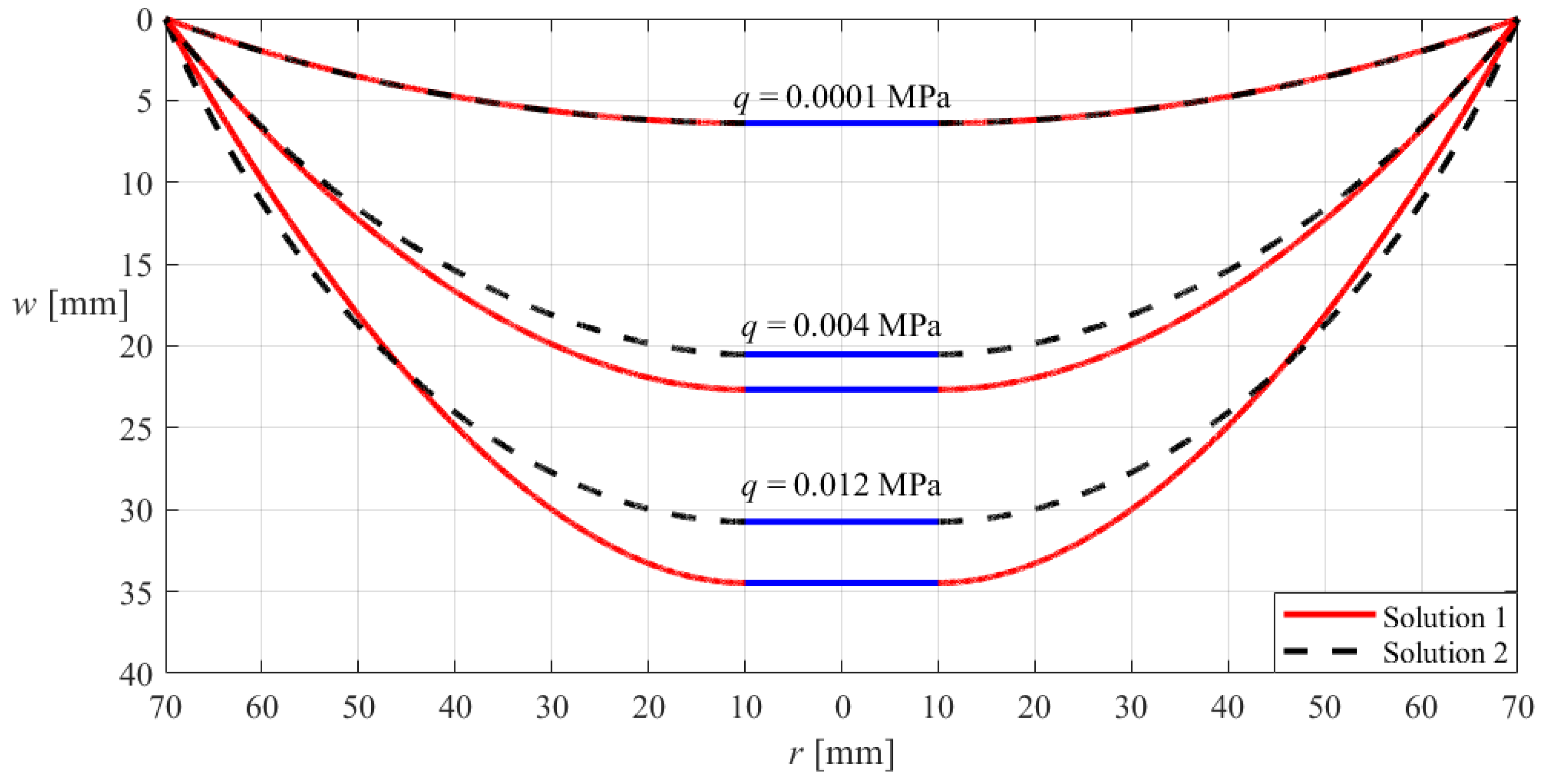
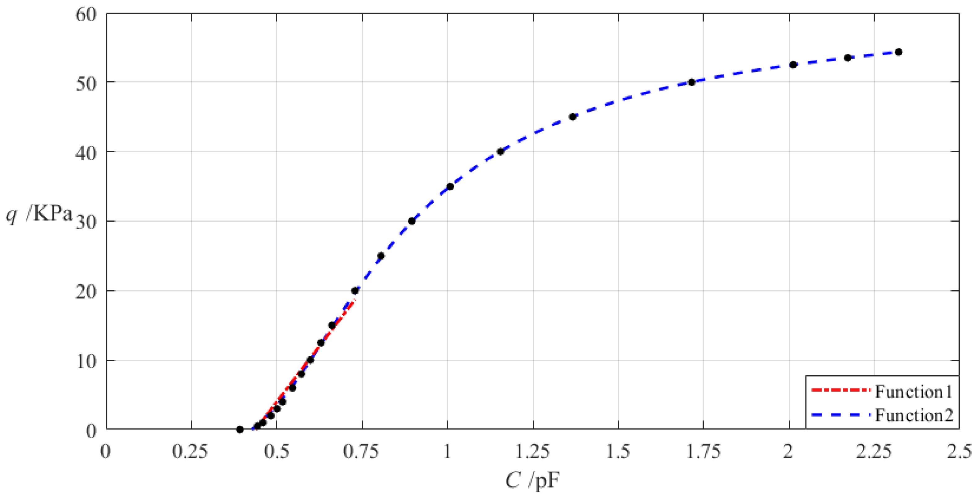
Appendix A
Table A1.
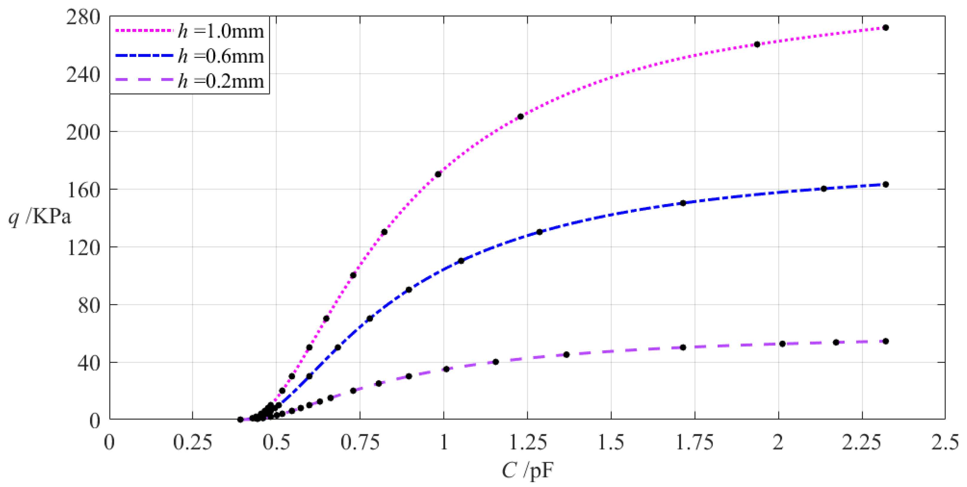
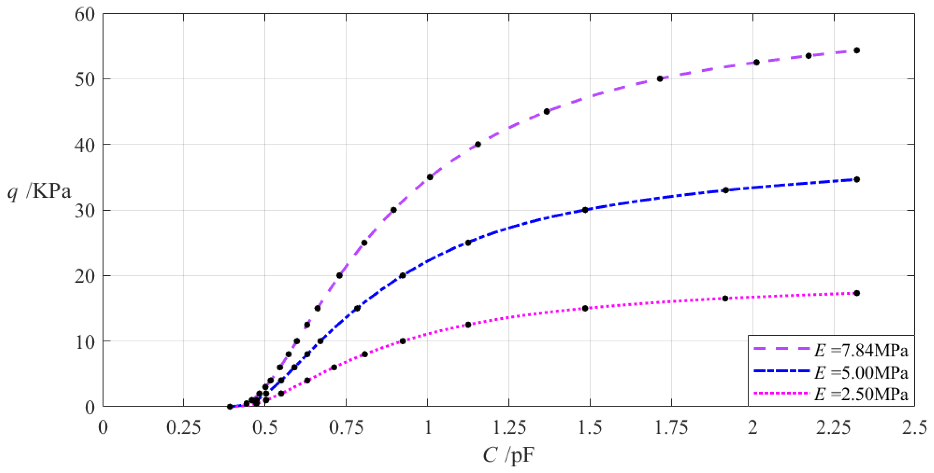
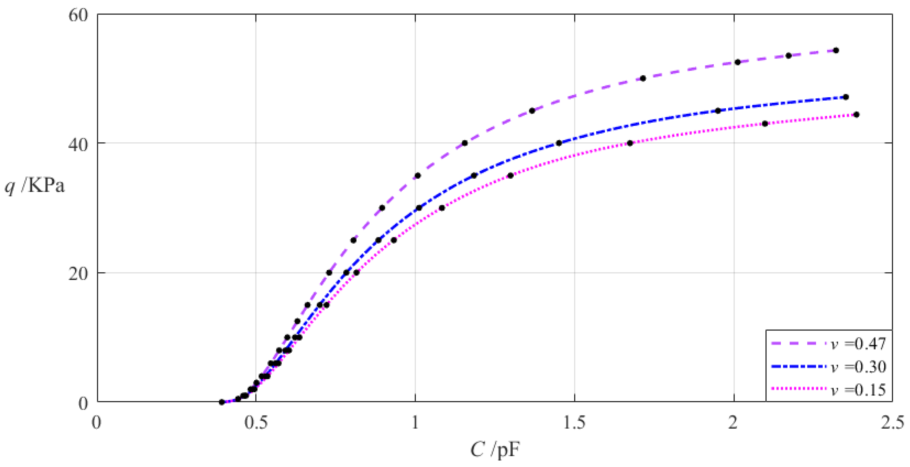
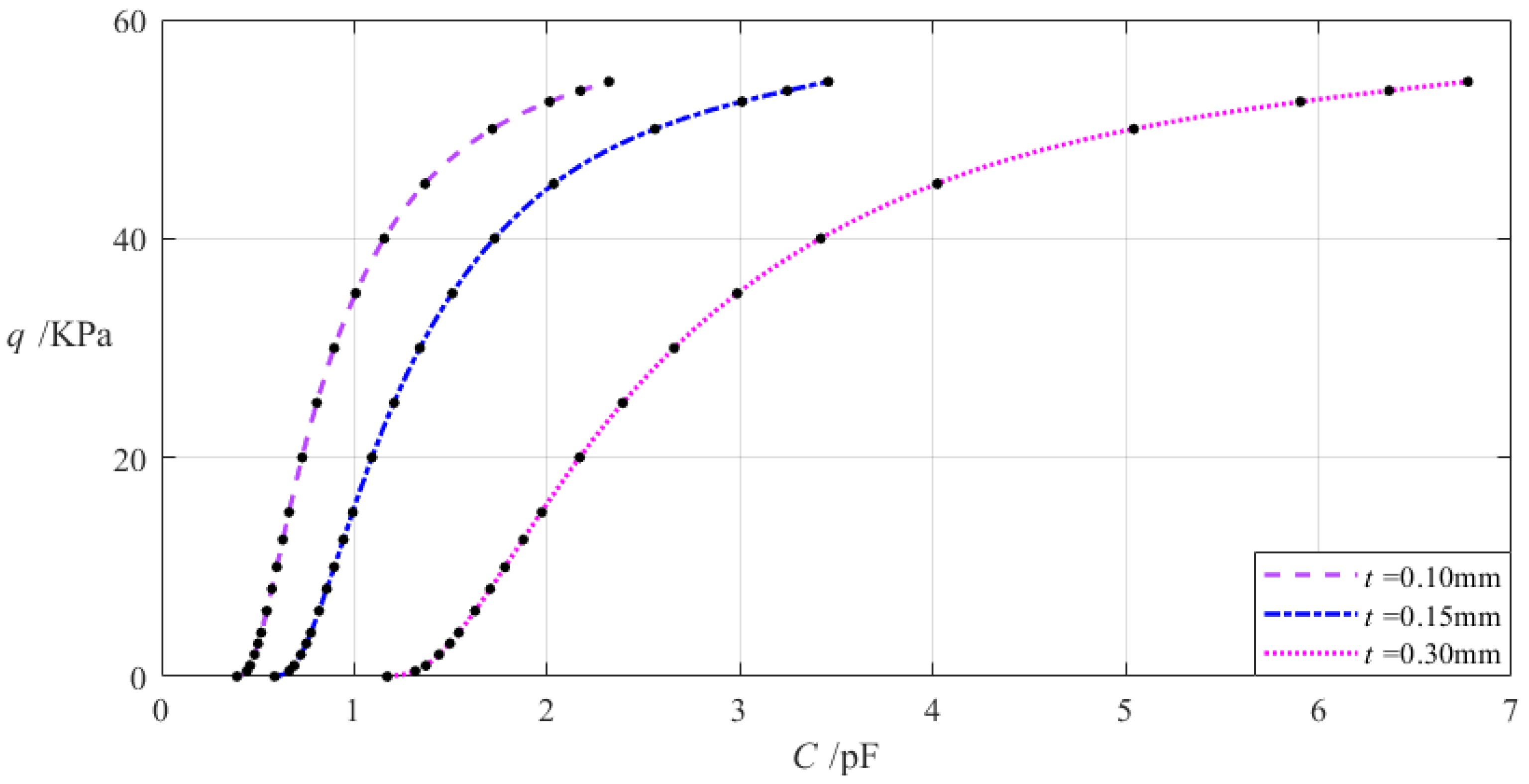
The numerical calculation results of the undetermined constants b0, c0, and d0, maximum membrane deflection wm, maximum membrane stress σm, and capacitance C when the uniformly distributed normal load q takes different values, and a = 70 mm, b = 50 mm, h = 0.2 mm, t = 0.1 mm, E = 7.84 MPa, ν = 0.47, and g = 17 mm.
Table A1.
The numerical calculation results of the undetermined constants b0, c0, and d0, maximum membrane deflection wm, maximum membrane stress σm, and capacitance C when the uniformly distributed normal load q takes different values, and a = 70 mm, b = 50 mm, h = 0.2 mm, t = 0.1 mm, E = 7.84 MPa, ν = 0.47, and g = 17 mm.
| q/KPa | b0 | c0 | d0 | wm/mm | σm/MPa | C/pF |
|---|
| 0 | 0 | 0 | 0 | 0 | 0 | 0.392 |
| 0.5 | 0.019743 | 0.011214 | 0.032027 | 2.992 | 0.167 | 0.443 |
| 1 | 0.031424 | 0.017831 | 0.040463 | 3.781 | 0.263 | 0.459 |
| 2 | 0.050091 | 0.028380 | 0.051207 | 4.787 | 0.415 | 0.483 |
| 3 | 0.065868 | 0.037270 | 0.058836 | 5.503 | 0.541 | 0.501 |
| 4 | 0.080043 | 0.045237 | 0.064973 | 6.080 | 0.652 | 0.517 |
| 6 | 0.105468 | 0.059481 | 0.074821 | 7.007 | 0.846 | 0.546 |
| 8 | 0.128394 | 0.072275 | 0.082795 | 7.759 | 1.017 | 0.572 |
| 10 | 0.149658 | 0.084099 | 0.089634 | 8.405 | 1.170 | 0.598 |
| 12.5 | 0.174562 | 0.097895 | 0.097121 | 9.115 | 1.346 | 0.629 |
| 15 | 0.198069 | 0.110866 | 0.103779 | 9.747 | 1.506 | 0.661 |
| 20 | 0.242049 | 0.135002 | 0.115417 | 10.856 | 1.794 | 0.729 |
| 25 | 0.283098 | 0.157374 | 0.125553 | 11.826 | 2.049 | 0.805 |
| 30 | 0.322015 | 0.178442 | 0.134679 | 12.703 | 2.278 | 0.896 |
| 35 | 0.359284 | 0.198489 | 0.143077 | 13.514 | 2.486 | 1.008 |
| 40 | 0.395229 | 0.217699 | 0.150927 | 14.274 | 2.678 | 1.155 |
| 45 | 0.430078 | 0.236206 | 0.158350 | 14.997 | 2.854 | 1.367 |
| 50 | 0.464001 | 0.254106 | 0.165433 | 15.689 | 3.017 | 1.715 |
| 52.5 | 0.479838 | 0.262150 | 0.168944 | 16.036 | 3.108 | 2.012 |
| 53.5 | 0.486457 | 0.265606 | 0.170283 | 16.168 | 3.138 | 2.172 |
| 54.3296 | 0.492803 | 0.269215 | 0.171299 | 16.265 | 3.150 | 2.321 |
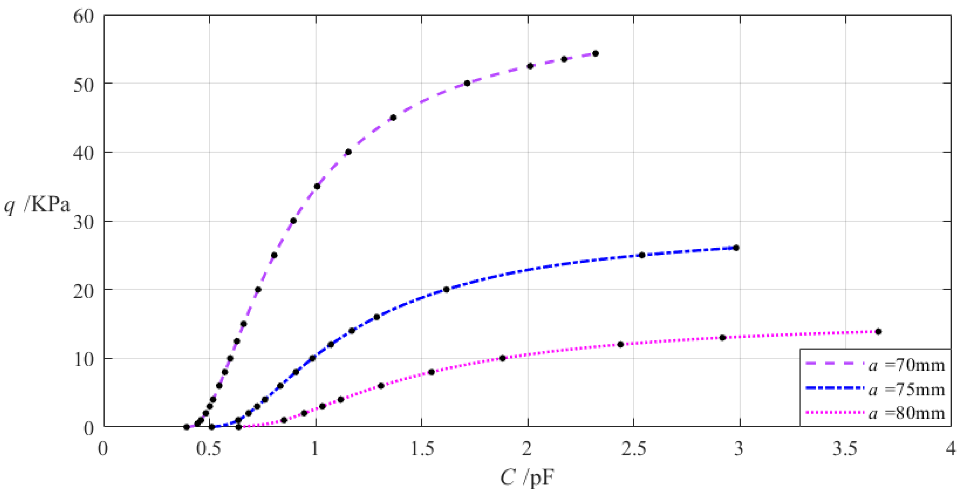
Table A2.
The numerical calculation results of the undetermined constants b0, c0, and d0, maximum membrane deflection wm, maximum membrane stress σm, and capacitance C when the uniformly distributed normal load q takes different values, and a = 75 mm, b = 50 mm, h = 0.2 mm, t = 0.1 mm, E = 7.84 MPa, ν = 0.47, and g = 17 mm.
| q/KPa | b0 | c0 | d0 | wm/mm | σm/MPa | C/pF |
|---|
| 0 | 0 | 0 | 0 | 0 | 0 | 0.510 |
| 1 | 0.036119 | 0.021189 | 0.050456 | 5.055 | 0.307 | 0.636 |
| 2 | 0.057596 | 0.033713 | 0.063885 | 6.405 | 0.483 | 0.684 |
| 3 | 0.075757 | 0.044263 | 0.073435 | 7.367 | 0.629 | 0.724 |
| 4 | 0.092082 | 0.053713 | 0.081129 | 8.144 | 0.757 | 0.762 |
| 6 | 0.121382 | 0.070596 | 0.093496 | 9.395 | 0.980 | 0.834 |
| 8 | 0.147819 | 0.085745 | 0.103534 | 10.414 | 1.175 | 0.907 |
| 10 | 0.172353 | 0.099732 | 0.112162 | 11.293 | 1.350 | 0.986 |
| 12 | 0.195495 | 0.112861 | 0.119832 | 12.076 | 1.511 | 1.072 |
| 14 | 0.217558 | 0.125321 | 0.126802 | 12.790 | 1.659 | 1.172 |
| 16 | 0.238752 | 0.137236 | 0.133234 | 13.450 | 1.798 | 1.289 |
| 20 | 0.279081 | 0.159764 | 0.144902 | 14.652 | 2.051 | 1.617 |
| 25 | 0.326552 | 0.186034 | 0.157890 | 15.998 | 2.332 | 2.539 |
| 26.0604 | 0.336283 | 0.191385 | 0.160472 | 16.265 | 2.387 | 2.983 |
Table A3.
The numerical calculation results of the undetermined constants b0, c0, and d0, maximum membrane deflection wm, maximum membrane stress σm, and capacitance C when the uniformly distributed normal load q takes different values, and a = 80 mm, b = 50 mm, h = 0.2 mm, t = 0.1 mm, E = 7.84 MPa, ν = 0.47, and g = 17 mm.
| q/KPa | b0 | c0 | d0 | wm/mm | σm/MPa | C/pF |
|---|
| 0 | 0 | 0 | 0 | 0 | 0 | 0.637 |
| 1 | 0.040419 | 0.024415 | 0.059873 | 6.403 | 0.348 | 0.851 |
| 2 | 0.064466 | 0.038832 | 0.075845 | 8.119 | 0.546 | 0.946 |
| 3 | 0.084810 | 0.050965 | 0.087217 | 9.344 | 0.710 | 1.032 |
| 4 | 0.103102 | 0.061825 | 0.096391 | 10.335 | 0.854 | 1.119 |
| 6 | 0.135945 | 0.081206 | 0.111161 | 11.935 | 1.104 | 1.309 |
| 8 | 0.165594 | 0.098572 | 0.123176 | 13.242 | 1.320 | 1.547 |
| 10 | 0.193119 | 0.114582 | 0.133527 | 14.373 | 1.514 | 1.882 |
| 12 | 0.219089 | 0.129590 | 0.142749 | 15.384 | 1.691 | 2.438 |
| 13 | 0.231606 | 0.136789 | 0.147037 | 15.855 | 1.774 | 2.919 |
| 13.8975 | 0.242593 | 0.143090 | 0.150727 | 16.265 | 1.845 | 3.655 |
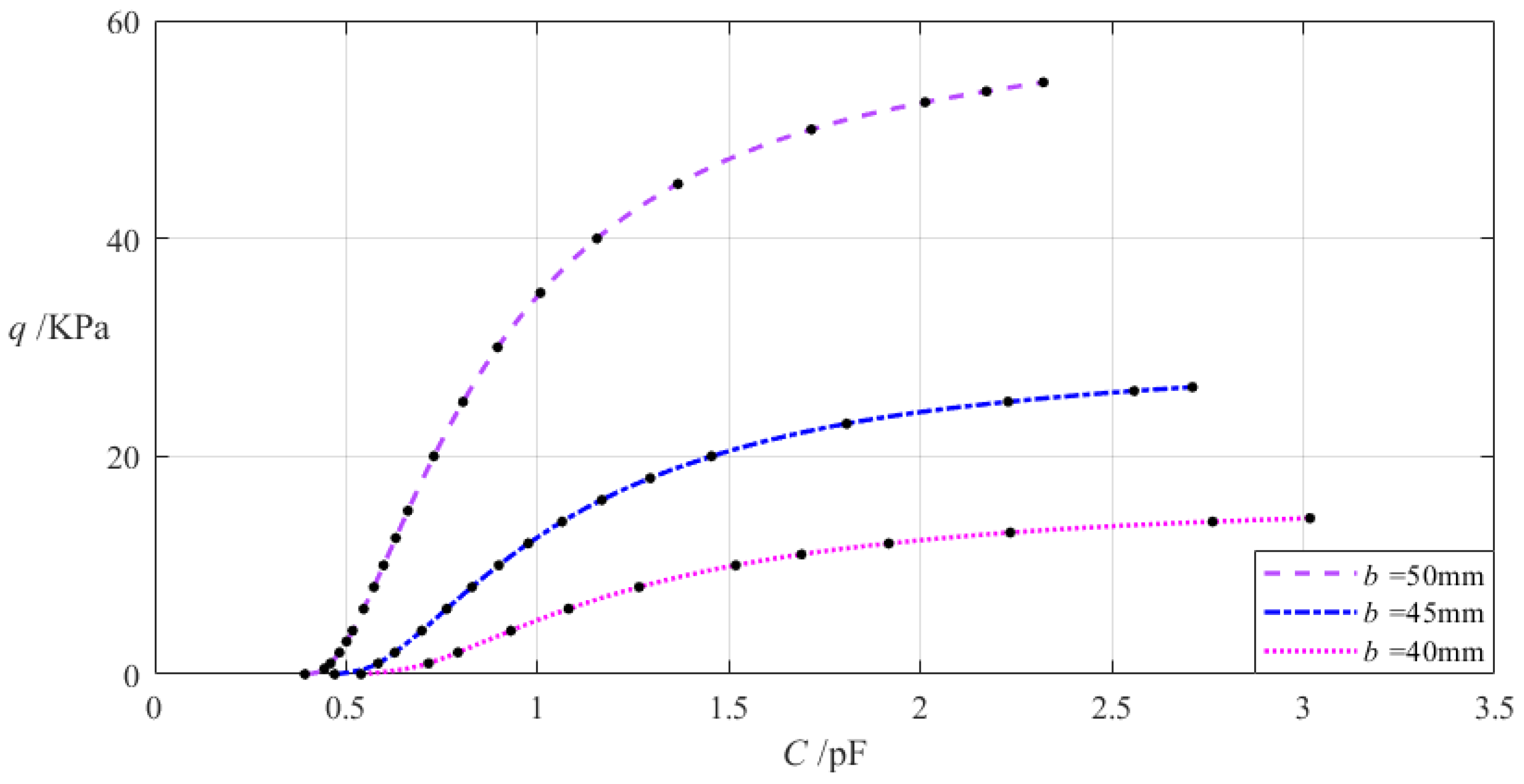
Table A4.
The numerical calculation results of the undetermined constants b0, c0, and d0, maximum membrane deflection wm, maximum membrane stress σm, and capacitance C when the uniformly distributed normal load q takes different values, and a = 70 mm, b = 45 mm, h = 0.2 mm, t = 0.1 mm, E = 7.84 MPa, ν = 0.47, and g = 17 mm.
| q/KPa | b0 | c0 | d0 | wm/mm | σm/MPa | C/pF |
|---|
| 0 | 0 | 0 | 0 | 0 | 0 | 0.470 |
| 1 | 0.035917 | 0.021431 | 0.053802 | 5.032 | 0.308 | 0.584 |
| 2 | 0.057262 | 0.034087 | 0.068115 | 6.376 | 0.484 | 0.627 |
| 4 | 0.091523 | 0.054277 | 0.086490 | 8.107 | 0.759 | 0.698 |
| 6 | 0.120616 | 0.071303 | 0.099662 | 9.352 | 0.982 | 0.763 |
| 8 | 0.146856 | 0.086565 | 0.110350 | 10.367 | 1.177 | 0.828 |
| 10 | 0.171198 | 0.100643 | 0.119536 | 11.241 | 1.352 | 0.899 |
| 12 | 0.194152 | 0.113848 | 0.127699 | 12.020 | 1.513 | 0.976 |
| 14 | 0.216028 | 0.126370 | 0.135117 | 12.730 | 1.661 | 1.064 |
| 16 | 0.237035 | 0.138335 | 0.141962 | 13.388 | 1.799 | 1.168 |
| 18 | 0.256855 | 0.149524 | 0.148447 | 14.008 | 1.930 | 1.294 |
| 20 | 0.276994 | 0.160932 | 0.154377 | 14.585 | 2.052 | 1.455 |
| 23 | 0.304995 | 0.176540 | 0.162910 | 15.407 | 2.228 | 1.807 |
| 25 | 0.324004 | 0.187241 | 0.168192 | 15.925 | 2.332 | 2.229 |
| 26 | 0.333091 | 0.192291 | 0.170784 | 16.177 | 2.383 | 2.558 |
| 26.3540 | 0.336286 | 0.194064 | 0.171690 | 16.265 | 2.402 | 2.711 |
Table A5.
The numerical calculation results of the undetermined constants b0, c0, and d0, maximum membrane deflection wm, maximum membrane stress σm, and capacitance C when the uniformly distributed normal load q takes different values, and a = 70 mm, b = 40 mm, h = 0.2 mm, t = 0.1 mm, E = 7.84 MPa, ν = 0.47, and g = 17 mm.
| q/KPa | b0 | c0 | d0 | wm/mm | σm/MPa | C/pF |
|---|
| 0 | 0 | 0 | 0 | 0 | 0 | 0.539 |
| 1 | 0.039854 | 0.025027 | 0.067629 | 6.334 | 0.350 | 0.715 |
| 2 | 0.063536 | 0.039767 | 0.085647 | 8.030 | 0.549 | 0.792 |
| 4 | 0.101542 | 0.063217 | 0.108809 | 10.221 | 0.858 | 0.931 |
| 6 | 0.133807 | 0.082925 | 0.125445 | 11.803 | 1.108 | 1.081 |
| 8 | 0.162903 | 0.100540 | 0.138969 | 13.095 | 1.325 | 1.265 |
| 10 | 0.189889 | 0.116740 | 0.150613 | 14.212 | 1.518 | 1.518 |
| 11 | 0.202511 | 0.124175 | 0.155891 | 14.710 | 1.607 | 1.689 |
| 12 | 0.215329 | 0.131892 | 0.160983 | 15.212 | 1.694 | 1.917 |
| 13 | 0.227277 | 0.138843 | 0.165745 | 15.661 | 1.776 | 2.234 |
| 14 | 0.239569 | 0.146219 | 0.170424 | 16.125 | 1.856 | 2.763 |
| 14.3232 | 0.243392 | 0.148468 | 0.171879 | 16.265 | 1.881 | 3.018 |
Table A6.
The numerical calculation results of the undetermined constants b0, c0, and d0, maximum membrane deflection wm, maximum membrane stress σm, and capacitance C when the uniformly distributed normal load q takes different values, and a = 70 mm, b = 50 mm, h = 0.6 mm, t = 0.1 mm, E = 7.84 MPa, ν = 0.47, and g = 17 mm.
| q/KPa | b0 | c0 | d0 | wm/mm | σm/MPa | C/pF |
|---|
| 0 | 0 | 0 | 0 | 0 | 0 | 0.392 |
| 1 | 0.015051 | 0.008552 | 0.027947 | 2.610 | 0.127 | 0.436 |
| 2 | 0.023940 | 0.013593 | 0.035285 | 3.296 | 0.202 | 0.449 |
| 4 | 0.038124 | 0.021622 | 0.044606 | 4.169 | 0.318 | 0.468 |
| 6 | 0.050091 | 0.028380 | 0.051206 | 4.787 | 0.415 | 0.483 |
| 8 | 0.060826 | 0.034431 | 0.056503 | 5.284 | 0.501 | 0.495 |
| 10 | 0.070737 | 0.040008 | 0.061008 | 5.707 | 0.579 | 0.506 |
| 30 | 0.149658 | 0.084099 | 0.089634 | 8.405 | 1.170 | 0.598 |
| 50 | 0.213125 | 0.119148 | 0.107870 | 10.136 | 1.606 | 0.683 |
| 70 | 0.269683 | 0.150079 | 0.122305 | 11.515 | 1.967 | 0.779 |
| 90 | 0.322015 | 0.178442 | 0.134679 | 12.703 | 2.278 | 0.896 |
| 110 | 0.371400 | 0.204978 | 0.145748 | 13.772 | 2.552 | 1.052 |
| 130 | 0.418572 | 0.230109 | 0.155917 | 14.760 | 2.797 | 1.286 |
| 150 | 0.464001 | 0.254106 | 0.165433 | 15.689 | 3.017 | 1.715 |
| 160 | 0.486166 | 0.265739 | 0.169998 | 16.137 | 3.119 | 2.136 |
| 162.9888 | 0.492803 | 0.269216 | 0.171299 | 16.265 | 3.150 | 2.321 |
Table A7.
The numerical calculation results of the undetermined constants b0, c0, and d0, maximum membrane deflection wm, maximum membrane stress σm, and capacitance C when the uniformly distributed normal load q takes different values, and a = 70 mm, b = 50 mm, h = 1 mm, t = 0.1 mm, E = 7.84 MPa, ν = 0.47, and g = 17 mm.
| q/KPa | b0 | c0 | d0 | wm/mm | σm/MPa | C/pF |
|---|
| 0 | 0 | 0 | 0 | 0.000 | 0.000 | 0.392 |
| 1 | 0.010697 | 0.006080 | 0.023546 | 2.199 | 0.091 | 0.428 |
| 2 | 0.017004 | 0.009661 | 0.029712 | 2.775 | 0.144 | 0.439 |
| 4 | 0.027053 | 0.015357 | 0.037524 | 3.506 | 0.227 | 0.454 |
| 6 | 0.035517 | 0.020148 | 0.043041 | 4.022 | 0.297 | 0.465 |
| 8 | 0.043100 | 0.024433 | 0.047457 | 4.436 | 0.359 | 0.474 |
| 10 | 0.050091 | 0.028380 | 0.051206 | 4.787 | 0.415 | 0.483 |
| 20 | 0.080043 | 0.045237 | 0.064973 | 6.080 | 0.652 | 0.517 |
| 30 | 0.105468 | 0.059481 | 0.074821 | 7.007 | 0.846 | 0.546 |
| 50 | 0.149658 | 0.084098 | 0.089634 | 8.405 | 1.170 | 0.598 |
| 70 | 0.188811 | 0.105763 | 0.101198 | 9.502 | 1.443 | 0.649 |
| 100 | 0.242049 | 0.135002 | 0.115417 | 10.856 | 1.794 | 0.729 |
| 130 | 0.291034 | 0.161681 | 0.127448 | 12.008 | 2.096 | 0.822 |
| 170 | 0.351945 | 0.194551 | 0.141446 | 13.356 | 2.446 | 0.983 |
| 210 | 0.409290 | 0.225180 | 0.153942 | 14.567 | 2.750 | 1.230 |
| 260 | 0.477340 | 0.261113 | 0.168186 | 15.959 | 3.079 | 1.936 |
| 271.6480 | 0.492803 | 0.269216 | 0.171299 | 16.265 | 3.150 | 2.321 |
Table A8.
The numerical calculation results of the undetermined constants b0, c0, and d0, maximum membrane deflection wm, maximum membrane stress σm, and capacitance C when the uniformly distributed normal load q takes different values, and a = 70 mm, b = 50 mm, h = 0.2 mm, t = 0.1 mm, E = 5 MPa, ν = 0.47, and g = 17 mm.
| q/KPa | b0 | c0 | d0 | wm/mm | σm/MPa | C/pF |
|---|
| 0 | 0 | 0 | 0 | 0 | 0 | 0.392 |
| 1 | 0.042517 | 0.024104 | 0.047132 | 4.405 | 0.226 | 0.473 |
| 2 | 0.067875 | 0.038398 | 0.059740 | 5.588 | 0.355 | 0.503 |
| 4 | 0.108708 | 0.061292 | 0.075992 | 7.117 | 0.555 | 0.550 |
| 6 | 0.143506 | 0.080682 | 0.087702 | 8.223 | 0.718 | 0.590 |
| 8 | 0.174987 | 0.098129 | 0.097244 | 9.126 | 0.860 | 0.630 |
| 10 | 0.204266 | 0.114277 | 0.105477 | 9.909 | 0.987 | 0.670 |
| 15 | 0.270626 | 0.150591 | 0.122879 | 11.570 | 1.261 | 0.784 |
| 20 | 0.332300 | 0.183987 | 0.137026 | 12.929 | 1.490 | 0.923 |
| 25 | 0.388743 | 0.214124 | 0.149912 | 14.178 | 1.694 | 1.125 |
| 30 | 0.444023 | 0.243578 | 0.161276 | 15.283 | 1.864 | 1.485 |
| 33 | 0.474816 | 0.259525 | 0.167924 | 15.936 | 1.967 | 1.918 |
| 34.6490 | 0.492803 | 0.269216 | 0.171299 | 16.265 | 2.009 | 2.321 |
Table A9.
The numerical calculation results of the undetermined constants b0, c0, and d0, maximum membrane deflection wm, maximum membrane stress σm, and capacitance C when the uniformly distributed normal load q takes different values, and a = 70 mm, b = 50 mm, h = 0.2 mm, t = 0.1 mm, E = 2.5 MPa, ν = 0.47, and g = 17 mm.
| q/KPa | b0 | c0 | d0 | wm/mm | σm/MPa | C/pF |
|---|
| 0 | 0 | 0 | 0 | 0 | 0 | 0.392 |
| 0.5 | 0.042517 | 0.024104 | 0.047132 | 4.405 | 0.113 | 0.473 |
| 1 | 0.067875 | 0.038398 | 0.059740 | 5.588 | 0.355 | 0.503 |
| 2 | 0.108708 | 0.061292 | 0.075992 | 7.117 | 0.555 | 0.550 |
| 4 | 0.174987 | 0.098129 | 0.097244 | 9.126 | 0.860 | 0.630 |
| 6 | 0.231939 | 0.129469 | 0.112822 | 10.608 | 0.551 | 0.712 |
| 8 | 0.283800 | 0.157755 | 0.125721 | 11.842 | 0.655 | 0.807 |
| 10 | 0.332300 | 0.183987 | 0.137026 | 12.929 | 0.745 | 0.923 |
| 12.5 | 0.388743 | 0.214124 | 0.149912 | 14.178 | 0.847 | 1.125 |
| 15 | 0.444023 | 0.243578 | 0.161276 | 15.283 | 0.932 | 1.485 |
| 16.5 | 0.474816 | 0.259525 | 0.167924 | 15.936 | 0.984 | 1.916 |
| 17.3245 | 0.492803 | 0.269216 | 0.171299 | 16.265 | 1.004 | 2.321 |
Table A10.
The numerical calculation results of the undetermined constants b0, c0, and d0, maximum membrane deflection wm, maximum membrane stress σm, and capacitance C when the uniformly distributed normal load q takes different values, and a = 70 mm, b = 50 mm, h = 0.2 mm, t = 0.1 mm, E = 7.84 MPa, ν = 0.3, and g = 17 mm.
| q/KPa | b0 | c0 | d0 | wm/mm | σm/MPa | C/pF |
|---|
| 0 | 0 | 0 | 0 | 0 | 0 | 0.392 |
| 1 | 0.029971 | 0.012548 | 0.043090 | 4.004 | 0.258 | 0.465 |
| 2 | 0.047823 | 0.019970 | 0.054553 | 5.071 | 0.407 | 0.490 |
| 4 | 0.076539 | 0.031832 | 0.069262 | 6.442 | 0.639 | 0.529 |
| 6 | 0.100982 | 0.041856 | 0.079800 | 7.427 | 0.830 | 0.561 |
| 8 | 0.123076 | 0.050860 | 0.088343 | 8.227 | 0.997 | 0.592 |
| 10 | 0.143611 | 0.059180 | 0.095677 | 8.914 | 1.149 | 0.622 |
| 15 | 0.189801 | 0.077769 | 0.111256 | 10.377 | 1.475 | 0.700 |
| 20 | 0.233293 | 0.095008 | 0.123391 | 11.523 | 1.763 | 0.783 |
| 25 | 0.272012 | 0.110212 | 0.135037 | 12.625 | 2.009 | 0.884 |
| 30 | 0.311452 | 0.125575 | 0.144169 | 13.492 | 2.241 | 1.012 |
| 35 | 0.346041 | 0.138781 | 0.154304 | 14.459 | 2.442 | 1.184 |
| 40 | 0.383377 | 0.153170 | 0.161764 | 15.171 | 2.639 | 1.451 |
| 45 | 0.415193 | 0.164903 | 0.171148 | 16.073 | 2.807 | 1.950 |
| 47.1070 | 0.431885 | 0.171497 | 0.173141 | 16.262 | 2.884 | 2.352 |
Table A11.
The numerical calculation results of the undetermined constants b0, c0, and d0, maximum membrane deflection wm, maximum membrane stress σm, and capacitance C when the uniformly distributed normal load q takes different values, and a = 70 mm, b = 50 mm, h = 0.2 mm, t = 0.1 mm, E = 7.84 MPa, ν = 0.15, and g = 17 mm.
| q/KPa | b0 | c0 | d0 | wm/mm | σm/MPa | C/pF |
|---|
| 0 | 0 | 0 | 0 | 0 | 0 | 0.392 |
| 1 | 0.029373 | 0.008294 | 0.044571 | 4.120 | 0.260 | 0.468 |
| 2 | 0.046905 | 0.013192 | 0.056436 | 5.218 | 0.410 | 0.494 |
| 4 | 0.075162 | 0.021005 | 0.071669 | 6.629 | 0.644 | 0.535 |
| 6 | 0.099268 | 0.027597 | 0.082585 | 7.642 | 0.837 | 0.570 |
| 8 | 0.121099 | 0.033510 | 0.091434 | 8.464 | 1.006 | 0.603 |
| 10 | 0.141424 | 0.038969 | 0.099031 | 9.170 | 1.159 | 0.636 |
| 15 | 0.186820 | 0.051064 | 0.115477 | 10.700 | 1.487 | 0.721 |
| 20 | 0.230552 | 0.062417 | 0.127718 | 11.844 | 1.785 | 0.815 |
| 25 | 0.268227 | 0.072109 | 0.140458 | 13.035 | 2.028 | 0.932 |
| 30 | 0.308638 | 0.082360 | 0.149210 | 13.856 | 2.278 | 1.084 |
| 35 | 0.341737 | 0.090496 | 0.160820 | 14.946 | 2.470 | 1.299 |
| 40 | 0.380749 | 0.100303 | 0.167416 | 15.567 | 2.691 | 1.674 |
| 43 | 0.397090 | 0.103956 | 0.175280 | 16.109 | 2.773 | 2.098 |
| 44.4034 | 0.411176 | 0.107736 | 0.174791 | 16.262 | 2.854 | 2.385 |
Table A12.
The numerical calculation results of the undetermined constants b0, c0, and d0, maximum membrane deflection wm, maximum membrane stress σm, and capacitance C when the uniformly distributed normal load q takes different values, and a = 70 mm, b = 50 mm, h = 0.2 mm, t = 0.15 mm, E = 7.84 MPa, ν = 0.47, and g = 17 mm.
| q/KPa | b0 | c0 | d0 | wm/mm | σm/MPa | C/pF |
|---|
| 0 | 0 | 0 | 0 | 0 | 0 | 0.587 |
| 0.5 | 0.019743 | 0.011214 | 0.032027 | 2.992 | 0.167 | 0.662 |
| 1 | 0.031424 | 0.017831 | 0.040463 | 3.781 | 0.263 | 0.688 |
| 2 | 0.050091 | 0.028380 | 0.051207 | 4.787 | 0.415 | 0.723 |
| 3 | 0.065868 | 0.037270 | 0.058836 | 5.503 | 0.541 | 0.751 |
| 4 | 0.080043 | 0.045237 | 0.064973 | 6.080 | 0.652 | 0.774 |
| 6 | 0.105468 | 0.059481 | 0.074821 | 7.007 | 0.846 | 0.817 |
| 8 | 0.128394 | 0.072275 | 0.082795 | 7.759 | 1.017 | 0.857 |
| 10 | 0.149658 | 0.084099 | 0.089634 | 8.405 | 1.170 | 0.895 |
| 12.5 | 0.174562 | 0.097895 | 0.097121 | 9.115 | 1.346 | 0.943 |
| 15 | 0.198069 | 0.110866 | 0.103779 | 9.747 | 1.506 | 0.992 |
| 20 | 0.242049 | 0.135002 | 0.115417 | 10.856 | 1.794 | 1.091 |
| 25 | 0.283098 | 0.157374 | 0.125553 | 11.826 | 2.049 | 1.207 |
| 30 | 0.322015 | 0.178442 | 0.134679 | 12.703 | 2.278 | 1.340 |
| 35 | 0.359284 | 0.198489 | 0.143077 | 13.514 | 2.486 | 1.509 |
| 40 | 0.395229 | 0.217699 | 0.150927 | 14.274 | 2.678 | 1.727 |
| 45 | 0.430078 | 0.236206 | 0.158350 | 14.997 | 2.854 | 2.034 |
| 50 | 0.464001 | 0.254106 | 0.165433 | 15.689 | 3.017 | 2.559 |
| 52.5 | 0.479838 | 0.262150 | 0.168944 | 16.036 | 3.108 | 3.010 |
| 53.5 | 0.486457 | 0.265606 | 0.170283 | 16.168 | 3.138 | 3.245 |
| 54.3296 | 0.492803 | 0.269215 | 0.171299 | 16.265 | 3.150 | 3.457 |
Table A13.
The numerical calculation results of the undetermined constants b0, c0, and d0, maximum membrane deflection wm, maximum membrane stress σm, and capacitance C when the uniformly distributed normal load q takes different values, and a = 70 mm, b = 50 mm, h = 0.2 mm, t = 0.3 mm, E = 7.84 MPa, ν = 0.47, and g = 17 mm.
| q/KPa | b0 | c0 | d0 | wm/mm | σm/MPa | C/pF |
|---|
| 0 | 0 | 0 | 0 | 0 | 0 | 1.170 |
| 0.5 | 0.019743 | 0.011214 | 0.032027 | 2.992 | 0.167 | 1.316 |
| 1 | 0.031424 | 0.017831 | 0.040463 | 3.781 | 0.263 | 1.371 |
| 2 | 0.050091 | 0.028380 | 0.051207 | 4.787 | 0.415 | 1.439 |
| 3 | 0.065868 | 0.037270 | 0.058836 | 5.503 | 0.541 | 1.495 |
| 4 | 0.080043 | 0.045237 | 0.064973 | 6.080 | 0.652 | 1.542 |
| 6 | 0.105468 | 0.059481 | 0.074821 | 7.007 | 0.846 | 1.627 |
| 8 | 0.128394 | 0.072275 | 0.082795 | 7.759 | 1.017 | 1.705 |
| 10 | 0.149658 | 0.084099 | 0.089634 | 8.405 | 1.170 | 1.781 |
| 12.5 | 0.174562 | 0.097895 | 0.097121 | 9.115 | 1.346 | 1.877 |
| 15 | 0.198069 | 0.110866 | 0.103779 | 9.747 | 1.506 | 1.972 |
| 20 | 0.242049 | 0.135002 | 0.115417 | 10.856 | 1.794 | 2.168 |
| 25 | 0.283098 | 0.157374 | 0.125553 | 11.826 | 2.049 | 2.392 |
| 30 | 0.322015 | 0.178442 | 0.134679 | 12.703 | 2.278 | 2.658 |
| 35 | 0.359284 | 0.198489 | 0.143077 | 13.514 | 2.486 | 2.986 |
| 40 | 0.395229 | 0.217699 | 0.150927 | 14.274 | 2.678 | 3.418 |
| 45 | 0.430078 | 0.236206 | 0.158350 | 14.997 | 2.854 | 4.023 |
| 50 | 0.464001 | 0.254106 | 0.165433 | 15.689 | 3.017 | 5.041 |
| 52.5 | 0.479838 | 0.262150 | 0.168944 | 16.036 | 3.108 | 5.906 |
| 53.5 | 0.486457 | 0.265606 | 0.170283 | 16.168 | 3.138 | 6.365 |
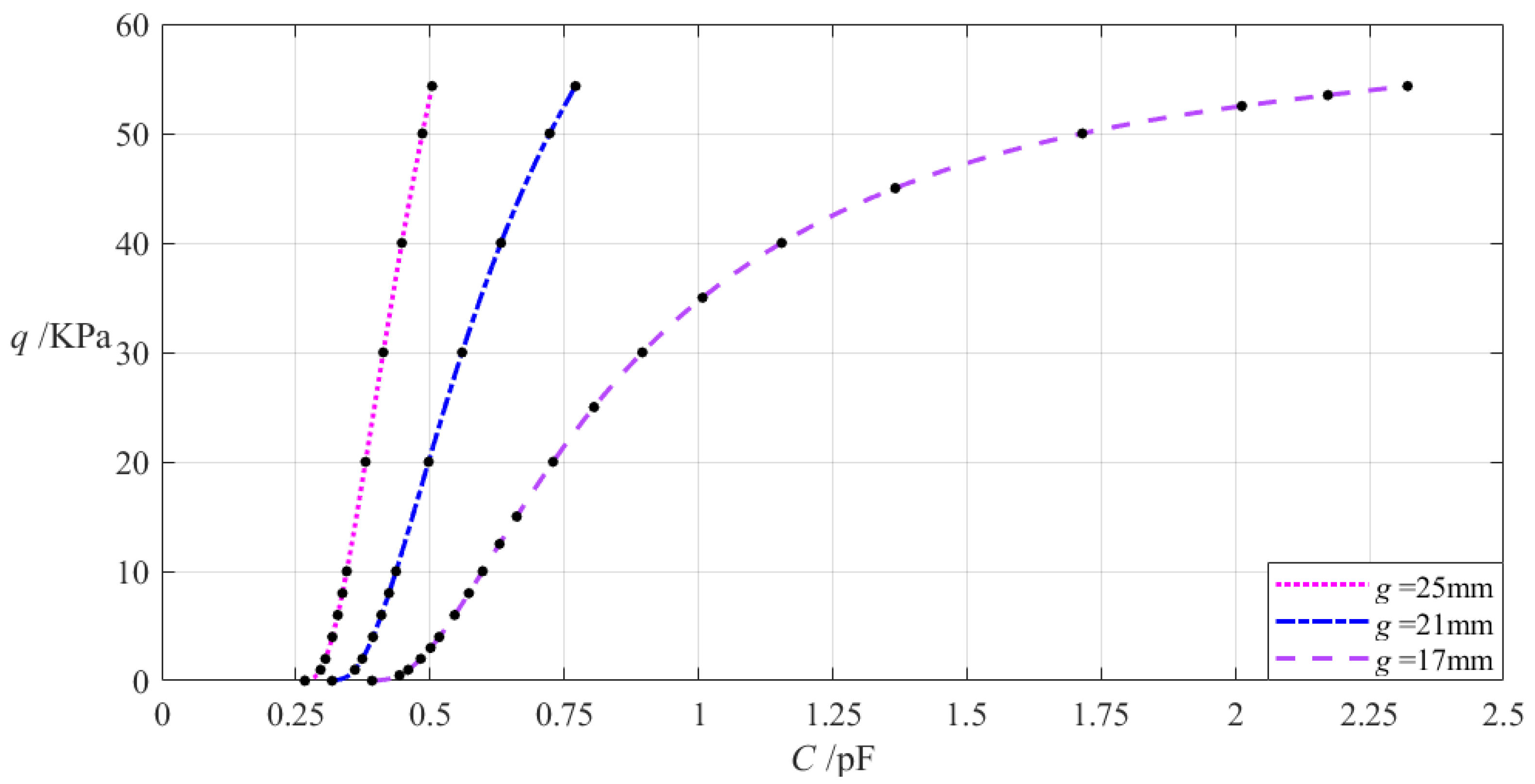
| 54.3296 | 0.492803 | 0.269215 | 0.171299 | 16.265 | 3.150 | 6.774 |
Table A14.
The numerical calculation results of the undetermined constants b0, c0, and d0, maximum membrane deflection wm, maximum membrane stress σm, and capacitance C when the uniformly distributed normal load q takes different values, and a = 70 mm, b = 50 mm, h = 0.2 mm, t = 0.1 mm, E = 7.84 MPa, ν = 0.47, and g = 21 mm.
| q/KPa | b0 | c0 | d0 | wm/mm | σm/MPa | C/pF |
|---|
| 0 | 0 | 0 | 0 | 0 | 0 | 0.317 |
| 1 | 0.031424 | 0.017831 | 0.040463 | 3.781 | 0.263 | 0.360 |
| 2 | 0.050091 | 0.028380 | 0.051207 | 4.787 | 0.415 | 0.374 |
| 4 | 0.080043 | 0.045237 | 0.064973 | 6.080 | 0.652 | 0.394 |
| 6 | 0.105468 | 0.059481 | 0.074821 | 7.007 | 0.846 | 0.409 |
| 8 | 0.128394 | 0.072275 | 0.082795 | 7.759 | 1.017 | 0.423 |
| 10 | 0.149658 | 0.084099 | 0.089634 | 8.405 | 1.170 | 0.437 |
| 20 | 0.242049 | 0.135002 | 0.115417 | 10.856 | 1.794 | 0.497 |
| 30 | 0.322015 | 0.178442 | 0.134679 | 12.703 | 2.278 | 0.560 |
| 40 | 0.395229 | 0.217699 | 0.150927 | 14.274 | 2.678 | 0.632 |
| 50 | 0.464001 | 0.254106 | 0.165433 | 15.689 | 3.017 | 0.723 |
| 54.3296 | 0.492803 | 0.269215 | 0.171299 | 16.265 | 3.150 | 0.771 |
Table A15.
The numerical calculation results of the undetermined constants b0, c0, and d0, maximum membrane deflection wm, maximum membrane stress σm, and capacitance C when the uniformly distributed normal load q takes different values, and a = 70 mm, b = 50 mm, h = 0.2 mm, t = 0.1 mm, E = 7.84 MPa, ν = 0.47, and g = 25 mm.
| q/KPa | b0 | c0 | d0 | wm/mm | σm/MPa | C/pF |
|---|
| 0 | 0 | 0 | 0 | 0 | 0 | 0.267 |
| 1 | 0.031424 | 0.017831 | 0.040463 | 3.781 | 0.263 | 0.296 |
| 2 | 0.050091 | 0.028380 | 0.051207 | 4.787 | 0.415 | 0.305 |
| 4 | 0.080043 | 0.045237 | 0.064973 | 6.080 | 0.652 | 0.318 |
| 6 | 0.105468 | 0.059481 | 0.074821 | 7.007 | 0.846 | 0.328 |
| 8 | 0.128394 | 0.072275 | 0.082795 | 7.759 | 1.017 | 0.337 |
| 10 | 0.149658 | 0.084099 | 0.089634 | 8.405 | 1.170 | 0.345 |
| 20 | 0.242049 | 0.135002 | 0.115417 | 10.856 | 1.794 | 0.380 |
| 30 | 0.322015 | 0.178442 | 0.134679 | 12.703 | 2.278 | 0.413 |
| 40 | 0.395229 | 0.217699 | 0.150927 | 14.274 | 2.678 | 0.447 |
| 50 | 0.464001 | 0.254106 | 0.165433 | 15.689 | 3.017 | 0.486 |
| 54.3296 | 0.492803 | 0.269215 | 0.171299 | 16.265 | 3.150 | 0.504 |


