Abstract
This paper presents efficient coupling methods that accurately reduce the computational cost for modelling solids dynamically with finite elements. A multi-time-step integration algorithm is developed to leverage varying time steps throughout a domain. Interfaces between subdomains are resolved explicitly with the continuity of acceleration and tractions. A spatial coupling method is combined with multiple time steps, allowing for meshes that do not necessarily conform at their interfaces. The method avoids solving additional degrees of freedom at these interfaces, with parameter-free coupling operators defined between meshes. A speedup >12× is achieved in comparison to reference single-time-step methods.
1. Introduction
The temporal and spatial discretisation of structural dynamic problems is directly related to the accuracy and computational cost of the explicit finite element method. Constrained by the Courant–Friedrichs–Lewy (CFL) condition, the critical time step, , is proportional to the element size, and inversely proportional to the dilatational wave speed [1]. This leads to simulations being restricted to of the element with the smallest size or highest wave speed. Initially referred to as subcycling, pioneering works allowed for the integration of multiple time steps in a single domain [2,3]. The coupling of various kinematic fields was explored, along with the stability of such algorithms [4,5]. Asynchronous variational integration is a non-trivial alternative, discretising the functional instead of the equations of motion [6]. The main drawback being its high complexity implementation. Heterogeneous asynchronous time integration extended methods to varying, non-integer and large time step ratios [7,8]. However, maintaining the continuity of kinematics at the interface remains a challenge, especially for all three fields [9]. In recent works, energy-conserving methods have been developed; however, they depart far from the CFL condition to resolve the interface conditions [10]. Spatially, non-matching mesh algorithms facilitate more flexible geometric modelling [11]. Nitsche’s method has shown to weakly enforce conditions on the interfaces of non-matching meshes without additional unknowns, but commonly suffers from sensitivity to parameters [12,13,14,15]. Following similar principles of weak continuity, Lagrange multipliers are called upon in the mortar-based methods [16,17,18,19,20]. These types of methods have proven to be very robust, however they struggle to fulfil the inf-sup stability condition, and incur a large computational cost with mapping master and slave nodes [21]. In comparison, the use of localised Lagrange multipliers introduces a frame that independently enforces compatibility constraints on each boundary [22,23,24,25,26,27]. However, as is common with other methods that introduce an additional discretised interface, the construction of this interface is neither trivial nor computationally cheap [28,29,30,31]. This brief review justifies the need for more efficient couplings, both temporally and spatially. Coupling algorithms that allow for varying time-step ratios, whilst stepping close to the CFL condition, concertedly those that solve for non-matching meshes, without increasing the degrees of freedom, remain a hot topic of research.
2. Governing Equations of Dynamic Solids
The problem of a solid body subject to impact is described through the partitioning of a domain as illustrated in Figure 1. The deformation is governed by the momentum balance equation acting on the solid domain :
where , , and denote the density, acceleration field, Cauchy stress tensor and body forces. Deformation is described at time for a specified constant . Updated Lagrangian formulations of a single body are found in the following [32,33,34]; here, we extend this to a partitioned formulation to solve multiple solid subdomains.
Figure 1.
A 3-D domain decomposed into and where and are coupling interfaces to be externally resolved on . Normal vector and tractions are visualised on and , respectively.
Defining multiple subdomains, we state is a solid body in an open region , with its boundary denoted . is partitioned into non-overlapping subdomains:
Starting from , for a two-subdomain partitioning, where and denote large and small subdomains. On the boundary of the two matching subdomains, , we enforce:
to ensure the continuity of acceleration and tractions , as well as enforcing Dirichlet and Neumann boundary conditions. The variational formulation of the dynamic equilibrium in Equation (1) can be described for both and as the following:
where we denote a variational velocity , in a space where , and as the rate of deformation. A discrete approximation of the variational form can be reduced to the following ordinary differential equations:
where for subdomains and , we sum, over a number of finite elements, and , in each subdomain:
The Lagrangian shape functions are represented by , with their derivatives denoted as . As is common within the explicit finite element method, is lumped for each subdomain, with and computed with vectors too. We elect to use the leapfrog time integration scheme to step through time, staggering the solution of each kinematic quantity such that:
noting that a diagonal mass matrix allows for a direct computation of acceleration. Velocity is computed on the half time step, with displacement found for each full time step. Next, we summarise the temporal coupling, enabled by multi-time-step (MTS) integration.
3. Multi-Time-Step Integration
Multi-time stepping enables partitioned subdomains and to integrate with and , respectively. However, to allow for this difference, special attention must be given to the solution of the interface . Crucially, the conditional stability of explicit methods requires an element’s time step to obey the CFL condition for a linear undamped system as follows:
Here, we represent as the critical time step, as the maximum eigenfrequency, as the characteristic length of an element e and the dilatational (longitudinal) wave speed.
3.1. Salient Multi-Time-Stepping Features
The asynchronous integration is enabled with three important groups of computations. The first is the explicit computation of the acceleration on the interface :
We define indicator matrices (vectors in 1-D) for each subdomain to identify the degrees of freedom on the interface of subdomains with dimensions for nodal number . These summations provide the ingredients for computing the interface acceleration:
where we compute at each large time step . The integration of the subdomains is controlled by the definition of the time-step ratios. Suppose the two subdomains begin at a similar point in time , where N and n are the small and large steps, respectively. The time after the maximum stable integration step (governed by the CFL condition) on each subdomain is referred to as the trial time , such that:
where for every , k small time steps elapse since the last point in time where subdomains are equal in time. Now we can define the current time-step ratio, , and next time-step ratio, for the advancement of with:
Starting from each common time step with the integration of , the number of small time steps is determined by the evaluation of time-step ratios and . If the condition of or ( and ) is satisfied, further steps on can proceed before integrating over . As a consequence of subdomains integrating over their own respective time step, we ensure that the proposed method still finds a common time between all subdomains. Following the small trial time exceeding the large trial time , the method computes two additional ratios and . These denote the reduction factors required to maintain the subdomains in synchronisation where . Hence:
Through computing on both subdomains, we can compare reduction factors, such that:
where we look to reduce the time step of the subdomain closest to the CFL condition. In the following section, we summarise the multi-time-stepping algorithm, with each of these key features, as well as its implementation.
3.2. Summary of Temporal Algorithm
We provide an overview of the method required to integrate and with and . It shows a single large step N, exemplifying each of the features mentioned above. Note that is used for when , and computation of in Equation (15) is only required at for a mass-conserving problem. One full loop of the procedure times is followed, with the subdomain synchronised after each large step N. The proposed method is implemented in an open-source python code, found in the following repository: https://github.com/kinfungchan/multi-time-step-integration (accessed on 9 December 2024) [35]. It contains re-implementations of methods from the literature for the two-subdomain cases [9,10]. Whilst we depict the case of just two subdomains, the Algorithm 1 can be extended to multiple by processing subdomains as pairs.
| Algorithm 1 Summary of Algorithm for Coupling in Time from N to |
|
3.3. Numerical Examples in Time
We present a numerical example in 1-D, with the elastic wave propagation through a heterogeneous bar. Suppose the domain is split into two subdomains and of similar discretisation, with isotropic elastic properties of GPa, GPa and kgmm−3. These material properties result in a non-integer , where the time-step ratio is solely driven by the dissimilar material properties. Figure 2 depicts the bar configuration. The velocity boundary condition is applied to at with ms−1, where we define a half sine wave with a frequency of rads−1. The difference in material impedance results in a portion of the incident wave being transmitted and the remainder reflected in the opposite direction.
Figure 2.
A one-dimensional heterogeneous domain split into a large subdomain and a small subdomain , solved with and , respectively, of length mm and mm. The problem assumes uni-axial motion with Poisson’s ratio . A compressive half sine velocity boundary condition is applied from .
In Figure 3, a comparison between the coupled solution ( with ) and the monolithic (single-time-step) solution is presented at four separate time stamps. The multi-time-step solution solves and over and , whereas is limited by . Consequently, for , our method reduces the number of integration steps on by half. From prescription of the full wave at , through to the transmission and reflection of the wave at , the MTS solution aligns very well with the single-time-step solution, despite halving the number of large time steps. This reduction in computational effort is even more prominent for highly heterogeneous configurations, as well as variance in spatial discretisation.
Figure 3.
Axial wave propagation in a heterogeneous bar: (a)—boundary condition at ms and initial transmission at ms of the stress wave; (b)—transmission and reflection of the stress wave at ms and ms.
For the above simulation, we also compute the energy components, at each small time step, of each subdomain with the following:
where n can be interchanged with N when evaluating . The balance of energy can be evaluated in a similar way to the works of Neal and Belytschko [3], with the following:
In Figure 4, we show each of the components of energy and its overall balance. For both monolithic and multi-time-step solutions, a smooth transition of energy is observed as the wave interacts with . Remarkably, as the temporal coupling is enforced, the for both and is of the order kNmm, significantly below each of the components at kNmm. This numerical example captures the propagation of a smooth pulse; however, severe loading cases, highly heterogeneous domains, and 3-D problems, with further details are provided in the following work [35].
4. Solving Non-Matching Meshes
The problem of non-matching meshes is commonly found when simulating the dynamical behaviour of solids. We present an algorithm, combined with multi-time stepping, that relaxes the constraint of these conforming nodes, allowing for a coarser representation of a subdomain to be utilised, hence reducing the computational overhead.
4.1. Combined Spatial and Temporal Coupling
The following section follows on from the governing equations defined in Section 2; however, we now allow for the non-overlapping interface to consist of two non-matching spatial discretisations. Their compatibility is maintained such that:
where positions use an incidence matrix, such that and for each subdomain, and the externally assembled interface contains to describe the common boundary between the subdomains. The total virtual power can be summated for two subdomains to give , where a general form is obtained:
where variations in velocity coupling force on the interface and are accounted for. and are interpolation (or prolongation) and incidence operators ( to ), respectively. To map to the interface, we describe this spatial coupling operator in more detail:
with dimensions determined by and , as the number of nodes on the interface of the subdomain and the number of nodes on the interface , respectively. Therefore, interpolates using Lagrangian shape functions for the two subdomains and :
where is viewed as a dirac Delta function for coincident nodes. It is convenient to define a restriction operator as the transpose of , to map both forces and mass from subdomain interfaces and onto . The summation on the interfaces now becomes:
where we compute mass , internal force and external force to allow for the explicit computation of in Equation (17) to be recalled. These operators are analogous to concepts in multigrid methods and localised Lagrange multipliers (LLMs) [36,37]. Subsequently, we map from , back to the subdomains’ interfaces:
We illustrate a non-matching mesh in Figure 5 and compute its operators through exemplifying a linear isoparametric mapping in 2-D, where is discretised with line elements to depict the simplicity of this coupling.
Figure 5.
A non-matching benchmark highlighting the interface with differently discretised subdomains partitioned with the large , small and externally meshed interface .
For the interpolation matrix, we elucidate that from to the mapping is simply one-to-one and will always take the form of an identity matrix , whereas requires computation of the shape functions:
where, for this example case, it can also be shown that the restriction is the transpose of the interpolation. The interface is assumed to share the same geometrical description on both subdomain interfaces and , without overlap or separation. The spatial and temporal methods are combined to give the following Algorithm 2:
| Algorithm 2 Summary of Non-Matching Mesh Algorithm with Multi-Time Stepping |
|
4.2. Numerical Examples in Space and Time
The following numerical study looks to represent the stress gradients prior to fracture in a compact-tension (CT) specimen test, utilising a similar geometry to the literature [38,39]. Figure 6a portrays the geometry modelled in the following example. As the specimen is loaded, stress concentrates about the specimen’s crack tip. We apply a ramped velocity boundary condition on nodes that create a semicircle for upper and lower pins, as shown in Figure 6b, with a maximum magnitude of 0.2 ms−1. Whilst uniformly distributed velocities are applied to each of the nodes in the pins, to replicate the contact pressure on the pins, methods such as those applied by Triclot et al. should be considered [40]. Material properties are similar to alumina with GPa, kgmm−3 and Poisson’s ratio . We model the CT specimen with three simulations: one using a fine mesh throughout the entire domain, one coupling a coarse and fine mesh with a single , and another with and integrating with multiple time steps and , respectively. Structured meshes are used in all cases where an element size of mm for fine and 1 mm for coarse. All simulations use , running for a maximum of ms.
Figure 6.
(a)—Diagram of compact-tension specimen with dimensions in [mm], as seen in Sommer et al. [39]; (b)—nodal sets on the meshed subdomain for prescribed velocity boundary conditions on top (+ve loading) and bottom (−ve loading) pins.
In Figure 7 and Figure 8, we plot the stress contours at ms and ms, respectively, where the stress concentration can be visualised at the crack tip of the specimen. Figure 7a and Figure 8a capture the reference mesh, whilst Figure 7b and Figure 8b capture the spatially coupled mesh on a single time step . Figure 8 accurately predicts maximum stresses of 0.0396 GPa vs. 0.0410 GPa for reference against non-matching mesh.
Figure 7.
Comparison of for (a) reference (monolithic) versus (b) spatially coupled dynamically loaded compact-tension specimen, clipping from −0.0005 to 0.01 GPa at ms.
Figure 8.
Comparison of for (a) reference (monolithic) versus (b) spatially coupled dynamically loaded compact-tension specimen, clipping from −0.0005 to 0.01 GPa at ms.
Further quantification on the performance of the non-matching mesh algorithm can be made with the evaluation of stress intensity factors, near the crack tip. Utilising the stress extrapolation method, stress values in the vicinity of the crack tip can be used to simultaneously solve for in-plane and shear factors [41,42]. In rectangular coordinates, these are given as follows:
where r represents the radial distance from the crack, and the angle relative to the crack plane. Whilst J-integral and virtual crack closure techniques (VCCTs) have been developed for more accurately evaluating K, here the consistency in the method for both reference and coupled solution proves a sufficient comparison [43,44]. The stress and in the nearest element to the crack correspond to Figure 9a where strong alignment between spatially coupled and reference solution can be observed. In Figure 9b, the analysis computes and with mm, , mm and with the slight variation in the spatial discretisation of and summarising in Table 1. and compute a difference of 3.5% and 6.3% in value when comparing uncoupled and coupled solutions. This is deemed reasonable granted the approximation of the stress extrapolation method. For future comparisons, the contribution of multiple Gauss integration points could be considered with the aforementioned J-integral or VCCT methods.
Figure 9.
(a): Stress evolution with crack tip at coordinates extrapolated from the nearest element comparing the reference (fine mesh) and coupled (coarse and fine mesh) simulation through time. (b): The crack tip where radius (r) and angle () are used to estimate stress intensity factor (SIF).
Table 1.
Comparison of stress intensity factors and for the compact-tension specimen test with reference mesh and spatially coupled mesh at final time ms.
Now with multi-time stepping, and step with ms and ms, producing a time-step ratio . Through combining spatial and temporal coupling, we observe similar (< GPa) results in distribution, as seen in Figure 10a. The difference in the coupled simulations is captured via Figure 10b, where the root mean square error (RMSE) is plotted. The stress is linearly interpolated for the non-matching mesh to allow for comparison of stress on the coarse mesh’s Gauss points. The couplings capture nearly the entire specimen within a <5% error. Considerable error is located around the circumference of the pins, where the chequerboard pattern indicates potential hourglassing in . To mitigate such issues, higher order or fully integrated elements could be used. However, in the presented results, we note that no hourglass control methods have been applied for fair comparison of the reference and coupled solutions. The other portion of error can be seen in the far right of the specimen in Figure 10; however, like the pins, these Gauss points reside far from the area of interest at the crack tip. To avoid such errors, a smaller element size would be required in ; however, this raises the trade-off between accuracy and computational efficiency. As per the temporal coupling, an energy balance in each of the two subdomains was achieved kNmm, orders of magnitude below individual components of energy. The computational efficiency is summarised with speedup achieved utilising both couplings, as presented in Table 2. Whilst a modest speedup is achieved with non-matching meshes, an even larger efficiency is found with coupling in both space and time. Considering that coupling with non-matching meshes and combined coupling in space and time result in similar accuracy, the addition of multi-time stepping to these simulations seems obvious.
Figure 10.
Comparison of for: (a)—combined spatial and temporal coupling (multi-time stepping); (b)—RMSE Error of for dynamically loaded compact-tension specimen at ms.
Table 2.
Computational runtimes and speedup vs. reference (single , of the dynamically loaded CT specimen. Reference mesh size is 0.58 mm throughout the domain, whereas coupled simulations utilise 0.58 and 1.0 mm for and , respectively. and used for temporally coupled run.
5. Conclusions
We present coupling methods for the dynamic modelling of solids with explicit finite elements, temporally and spatially. When modelling composites, constituents have varying dilatational wave speeds, hence different time steps. Integrating over the smallest time step can prove highly inefficient, hence the need for multi-time stepping. Our method allows partitions of a domain to solve with their own respective time step, regardless of time-step ratio, hence reducing computational overhead. The method avoids solving a system of equations on the interface, unlike many of the methods that employ Lagrange multipliers. The stability of the method is assessed through evaluation of the subdomains’ energy balance. Very-high-frequency content or variations in motion below the time step of elements on the interface could result in spurious oscillations being generated. This potential limitation promotes the development of adaptive multi-time-stepping schemes that maintain the stability of the interface, withstanding high-frequency stress waves.
The addition of the coupling in space solves the issue of non-matching meshes so that small element sizes are only required in regions of interest. Coupling operators are easily implemented, without increasing the degrees of freedom on the interface. The method avoids the storage of large sparse matrices, reducing computational memory requirements. Ongoing work addresses the spatial coupling with quadrilateral non-matching interfaces in 3-D domains [45]. Numerical examples capture an increase in efficiency with stress wave propagation in a heterogeneous bar, and the modelling of a compact-tension specimen. Both couplings in time and space reduce computational runtimes when compared to their monolithic simulation, especially when combined. Limitations that concern the combination of spatial and temporal coupling include the computation of operators and solely at . Whilst this suffices for the benchmarks shown, for larger deformations this assumption is likely to require further development. Geometric representations of a non-matching that are non-planar have still yet to be explored. This proves an important topic as these couplings are applied to real-world multi-scale problems.
Future work looks at the coupling between macro- and meso-scale meshes [46,47,48], with adaptivity a clear necessity for these multi-scale couplings [49]. Whilst linear elasticity is a fair assumption for the rates of deformation demonstrated, other constitutive models should be investigated to evaluate the performance of the couplings, with further reductions in time steps and element distortion. In parallel, experimental fields that require efficiently capturing wave propagation with explicit finite elements are widespread [50,51]. Other coupling opportunities are plentiful when considering dynamic applications; the modelling of contact [14,16], composite fractures [38,39], fluid–structure interactions [13,27], and other impact engineering scenarios are just a few worth mentioning.
Author Contributions
Conceptualization, K.F.C., N.B. and N.P.; Methodology, K.F.C., N.B., I.S., S.F. and N.P.; Software, K.F.C., N.B., I.S. and S.F.; Validation, K.F.C.; Investigation, K.F.C. and N.B.; Writing—review & editing, N.B., I.S. and S.F.; Supervision, N.B. and N.P.; Project administration, N.P.; Funding acquisition, N.P. All authors have read and agreed to the published version of the manuscript.
Funding
This research was funded by the Engineering and Physical Sciences Research Council (EPSRC) and Rolls-Royce’s ASiMoV Prosperity Partnership with Reference EP/S005072/1.
Institutional Review Board Statement
Not applicable.
Informed Consent Statement
Not applicable.
Data Availability Statement
The original contributions presented in the study are included in the article, further inquiries can be directed to the corresponding author.
Acknowledgments
The authors would like to thank the reviewers for their helpful comments for improving this manuscript.
Conflicts of Interest
Author Nicola Bombace was employed by the company Advanced Micro Devices Inc. The remaining authors declare that the research was conducted in the absence of any commercial or financial relationships that could be construed as a potential conflict of interest.
References
- Courant, R.; Friedrichs, K.; Lewy, H. On the partial difference equations of mathematical physics. IBM J. Res. Dev. 1967, 11, 215–234. [Google Scholar] [CrossRef]
- Hughes, T.J.; Liu, W.K. Implicit-explicit finite elements in transient analysis: Implementation and numerical examples. J. Appl. Mech. Trans. ASME 1978, 45, 375–378. [Google Scholar] [CrossRef]
- Neal, M.O.; Belytschko, T. Explicit-explicit subcycling with non-integer time step ratios for structural dynamic systems. Comput. Struct. 1989, 31, 871–880. [Google Scholar] [CrossRef]
- Daniel, W.J.T. Analysis and implementation of a new constant acceleration subcycling algorithm. Int. J. Numer. Methods Eng. 1997, 40, 2841–2855. [Google Scholar] [CrossRef]
- Daniel, W.J.T. A partial velocity approach to subcycling structural dynamics. Comput. Methods Appl. Mech. Eng. 2003, 192, 375–394. [Google Scholar] [CrossRef]
- Lew, A.; Marsden, J.E.; Ortiz, M.; West, M. Variational time integrators. Int. J. Numer. Methods Eng. 2004, 60, 153–212. [Google Scholar] [CrossRef]
- Combescure, A.; Gravouil, A. A numerical scheme to couple subdomains with different time-steps for predominantly linear transient analysis. Comput. Methods Appl. Mech. Eng. 2002, 191, 1129–1157. [Google Scholar] [CrossRef]
- Gravouil, A.; Combescure, A.; Brun, M. Heterogeneous asynchronous time integrators for computational structural dynamics. Int. J. Numer. Methods Eng. 2015, 102, 202–232. [Google Scholar] [CrossRef]
- Cho, S.S.; Kolman, R.; González, J.A.; Park, K.C. Explicit multistep time integration for discontinuous elastic stress wave propagation in heterogeneous solids. Int. J. Numer. Methods Eng. 2019, 118, 276–302. [Google Scholar] [CrossRef]
- Dvořák, R.; Kolman, R.; Mračko, M.; Kopačka, J.; Fíla, T.; Jiroušek, O.; Falta, J.; Neuhäuserová, M.; Rada, V.; Adámek, V.; et al. Energy-conserving interface dynamics with asynchronous direct time integration employing arbitrary time steps. Comput. Methods Appl. Mech. Eng. 2023, 413, 116110. [Google Scholar] [CrossRef]
- de Boer, A.; van Zuijlen, A.H.; Bijl, H. Review of coupling methods for non-matching meshes. Comput. Methods Appl. Mech. Eng. 2007, 196, 1515–1525. [Google Scholar] [CrossRef]
- Hansbo, A.; Hansbo, P. An unfitted finite element method, based on Nitsche’s method, for elliptic interface problems. Comput. Methods Appl. Mech. Eng. 2002, 191, 5537–5552. [Google Scholar] [CrossRef]
- Hansbo, A.; Hansbo, P. Nitsche’s method for coupling non-matching meshes in fluid-structure vibration problems. Comput. Mech. 2002, 32, 134–139. [Google Scholar] [CrossRef]
- Wriggers, P.; Zavarise, G. A formulation for frictionless contact problems using a weak form introduced by Nitsche. Comput. Mech. 2017, 41, 407–420. [Google Scholar] [CrossRef]
- Sanders, J.D.; Laursen, T.A.; Puso, M.A. A Nitsche embedded mesh method. Comput. Mech. 2010, 49, 243–257. [Google Scholar] [CrossRef]
- Puso, M.A.; Laursen, T.A. A mortar segment-to-segment contact method for large deformation solid mechanics. Comput. Methods Appl. Mech. Eng. 2004, 193, 601–629. [Google Scholar] [CrossRef]
- Faucher, V.; Combescure, A. A time and space mortar method for coupling linear modal subdomains and non-linear subdomains in explicit structural dynamics. Comput. Methods Appl. Mech. Eng. 2003, 192, 509–533. [Google Scholar] [CrossRef]
- Steinbrecher, I.; Mayr, M.; Grill, M.J.; Kremheller, J.; Meier, C.; Popp, A. A mortar-type finite element approach for embedding 1D beams into 3D solid volumes. Comput. Mech. 2020, 66, 1377–1398. [Google Scholar] [CrossRef]
- Zhou, M.; Zhang, B.; Chen, T.; Peng, C.; Fang, H. A three-field dual mortar method for elastic problems with nonconforming mesh. Comput. Methods Appl. Mech. Eng. 2020, 362, 112870. [Google Scholar] [CrossRef]
- Wilson, P.; Teschemacher, T.; Bucher, P.; Wüchner, R. Non-conforming FEM-FEM coupling approaches and their application to dynamic structural analysis. Eng. Struct. 2021, 241, 112342. [Google Scholar] [CrossRef]
- Singer, V.; Teschemacher, T.; Larese, A.; Wüchner, R.; Bletzinger, K.U. Lagrange multiplier imposition of non-conforming essential boundary conditions in implicit material point method. Comput. Mech. 2024, 73, 1311–1333. [Google Scholar] [CrossRef]
- Puso, M.A.; Laursen, T.A. A simple algorithm for localized construction of non-matching structural interfaces. Int. J. Numer. Methods Eng. 2002, 53, 2117–2142. [Google Scholar]
- Herry, B.; Di Valentin, L.; Combescure, A. An approach to the connection between subdomains with non-matching meshes for transient mechanical analysis. Int. J. Numer. Methods Eng. 2002, 55, 973–1003. [Google Scholar] [CrossRef]
- Subber, W.; Matouš, K. Asynchronous space–time algorithm based on a domain decomposition method for structural dynamics problems on non-matching meshes. Comput. Mech. 2016, 57, 211–235. [Google Scholar]
- González, J.A.; Kolman, R.; Cho, S.S.; Felippa, C.A.; Park, K.C. Inverse mass matrix via the method of localized Lagrange multipliers. Int. J. Numer. Methods Eng. 2018, 113, 277–295. [Google Scholar] [CrossRef]
- Jeong, G.E.; Song, Y.U.; Youn, S.K.; Park, K.C. A new approach for nonmatching interface construction by the method of localized Lagrange multipliers. Comput. Methods Appl. Mech. Eng. 2020, 361, 112728. [Google Scholar] [CrossRef]
- González, J.A.; Park, K.C. Three-field partitioned analysis of fluid–structure interaction problems with a consistent interface model. Comput. Methods Appl. Mech. Eng. 2023, 414, 116134. [Google Scholar] [CrossRef]
- Cho, Y.S.; Jun, S.; Im, S.; Kim, H.G. An improved interface element with variable nodes for non-matching finite element meshes. Comput. Methods Appl. Mech. Eng. 2005, 194, 3022–3046. [Google Scholar] [CrossRef]
- Kim, H.G. Development of three-dimensional interface elements for coupling of non-matching hexahedral meshes. Comput. Methods Appl. Mech. Eng. 2005, 197, 3870–3882. [Google Scholar] [CrossRef]
- Bitencourt, L.A., Jr.; Manzoli, O.L.; Prazeres, P.G.; Rodrigues, E.A.; Bittencourt, T.N. A coupling technique for non-matching finite element meshes. Comput. Methods Appl. Mech. Eng. 2015, 290, 19–44. [Google Scholar] [CrossRef]
- Rodrigues, E.A.; Manzoli, O.L.; Bitencourt, L.A., Jr.; Bittencourt, T.N.; Sánchez, M. An adaptive concurrent multiscale model for concrete based on coupling finite elements. Comput. Methods Appl. Mech. Eng. 2018, 328, 26–46. [Google Scholar] [CrossRef]
- Dunne, F.; Petrinic, N. Introduction to Computational Plasticity; OUP: Oxford, UK, 2005. [Google Scholar]
- de Souza Neto, E.A.; Peric, D.; Owen, D.R. Computational Methods for Plasticity: Theory and Applications; John Wiley & Sons: Hoboken, NJ, USA, 2011. [Google Scholar]
- Belytschko, T.; Liu, W.K.; Moran, B.; Elkhodary, K. Nonlinear Finite Elements for Continua and Structures; John Wiley & Sons: Hoboken, NJ, USA, 2014. [Google Scholar]
- Chan, K.F.; Bombace, N.; Sap, D.; Wason, D.; Falco, S.; Petrinic, N. A Multi-Time Stepping Algorithm for the Modelling of Heterogeneous Structures With Explicit Time Integration. Int. J. Numer. Methods Eng. 2025, 126, e7638. [Google Scholar] [CrossRef]
- Biotteau, E.; Gravouil, A.; Lubrecht, A.A.; Combescure, A. Multigrid solver with automatic mesh refinement for transient elastoplastic dynamic problems. Int. J. Numer. Methods Eng. 2010, 84, 947–971. [Google Scholar] [CrossRef]
- Dvořák, R.; Kolman, R.; González, J.A. On the automatic construction of interface coupling operators for non-matching meshes by optimization methods. Comput. Methods Appl. Mech. Eng. 2024, 432, 117336. [Google Scholar] [CrossRef]
- Pinho, S.T.; Robinson, P.; Iannucci, L. Fracture toughness of the tensile and compressive fibre failure modes in laminated composites. Compos. Sci. Technol. 2006, 66, 2069–2079. [Google Scholar]
- Sommer, D.E.; Thomson, D.; Hoffmann, J.; Petrinic, N. Numerical modelling of quasi-static and dynamic compact tension tests for obtaining the translaminar fracture toughness of CFRP. Compos. Sci. Technol. 2023, 237, 109997. [Google Scholar] [CrossRef]
- Triclot, J.; Corre, T.; Gravouil, A.; Lazarus, V. Key role of boundary conditions for the 2D modeling of crack propagation in linear elastic Compact Tension tests. Eng. Fract. Mech. 2023, 277, 109012. [Google Scholar] [CrossRef]
- Han, Q.; Wang, Y.; Yin, Y.; Wang, D. Determination of stress intensity factor for mode I fatigue crack based on finite element analysis. Eng. Fract. Mech. 2015, 138, 118–126. [Google Scholar] [CrossRef]
- Qian, G.; González-Albuixech, V.F.; Niffenegger, M.; Giner, E. Comparison of KI calculation methods. Eng. Fract. Mech. 2016, 156, 52–67. [Google Scholar] [CrossRef]
- Zhao, X.; Mo, Z.L.; Guo, Z.Y.; Li, J. A modified three-dimensional virtual crack closure technique for calculating stress intensity factors with arbitrarily shaped finite element mesh arrangements across the crack front. Theor. Appl. Fract. Mech. 2020, 109, 102695. [Google Scholar] [CrossRef]
- Courtin, S.; Gardin, C.; Bezine, G.; Hamouda, H.B.H. Advantages of the J-integral approach for calculating stress intensity factors when using the commercial finite element software ABAQUS. Eng. Fract. Mech. 2005, 72, 2174–2185. [Google Scholar] [CrossRef]
- Sahu, I. Bilinear-Inverse-Mapper: Analytical Solution and Algorithm for Inverse Mapping of Bilinear Interpolation of Quadrilaterals. SSRN 2024, 4790071. Available online: https://ssrn.com/abstract=4790071 (accessed on 9 December 2024). [CrossRef]
- Falco, S.; Fogell, N.; Iannucci, L.; Petrinic, N.; Eakins, D. A method for the generation of 3D representative models of granular based materials. Int. J. Numer. Methods Eng. 2017, 112, 338–359. [Google Scholar] [CrossRef]
- Wason, D. A Multi-Scale Approach to the Development of High-Rate-Based Microstructure-Aware Constitutive Models for Magnesium Alloys. Ph.D. Thesis, University of Oxford, Oxford, UK, 2023. [Google Scholar]
- Falco, S.; Fogell, N.; Iannucci, L.; Petrinic, N.; Eakins, D. Raster approach to modelling the failure of arbitrarily inclined interfaces with structured meshes. Comput. Mech. 2024, 74, 805–818. [Google Scholar] [CrossRef]
- Bombace, N. Dynamic Adaptive Concurrent Multi-Scale Simulation of Wave Propagation in 3D Media. Doctoral dissertation. Ph.D. Thesis, University of Oxford, Oxford, UK, 2018. [Google Scholar]
- Martínez-Hergueta, F.; Pellegrino, A.; Ridruejo, Á.; Petrinic, N.; González, C.; LLorca, J. Dynamic tensile testing of needle-punched nonwoven fabrics. Appl. Sci. 2020, 10, 5081. [Google Scholar] [CrossRef]
- Tserpes, K.; Kormpos, P. Detailed Finite Element Models for the Simulation of the Laser Shock Wave Response of 3D Woven Composites. J. Compos. Sci. 2024, 8, 83. [Google Scholar] [CrossRef]
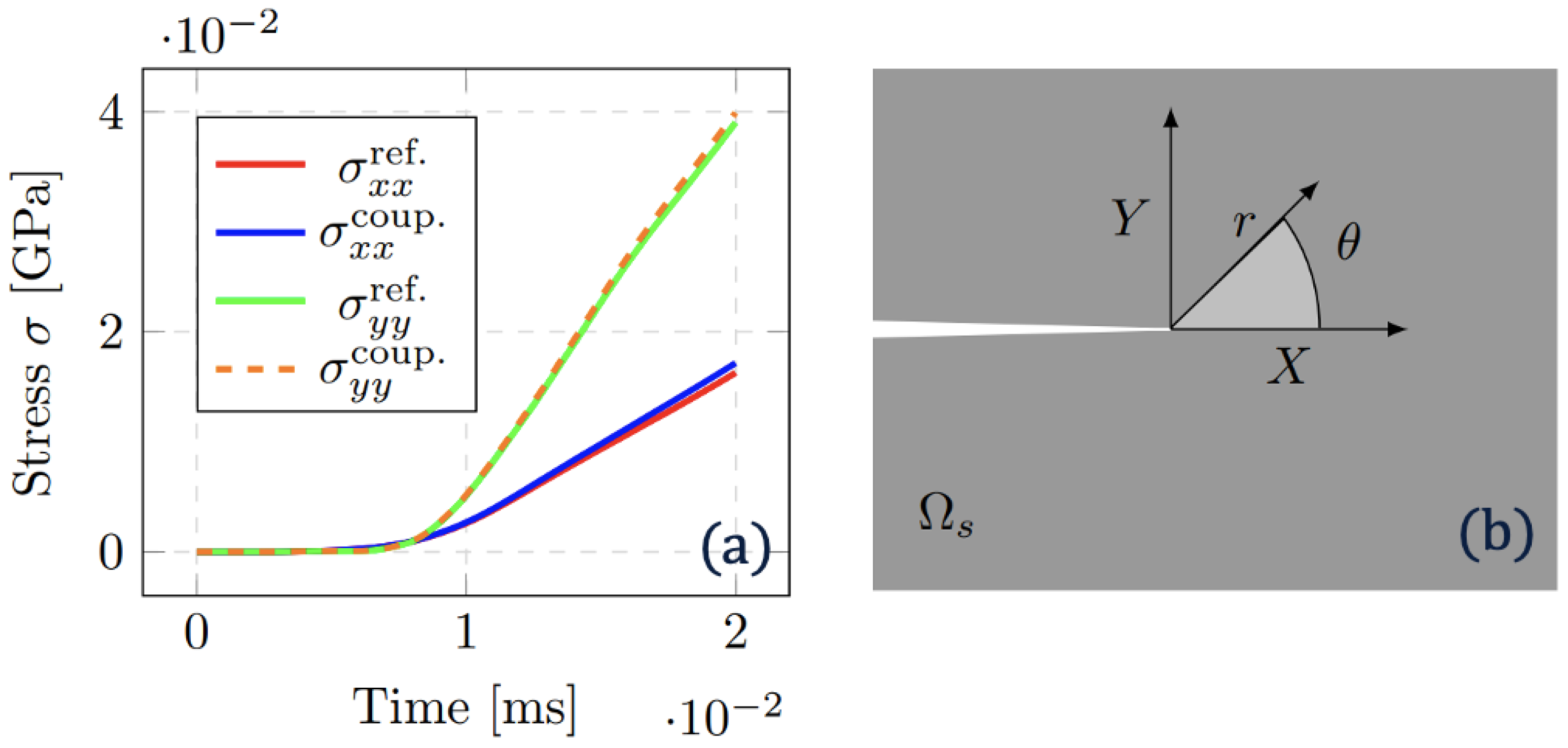
Disclaimer/Publisher’s Note: The statements, opinions and data contained in all publications are solely those of the individual author(s) and contributor(s) and not of MDPI and/or the editor(s). MDPI and/or the editor(s) disclaim responsibility for any injury to people or property resulting from any ideas, methods, instructions or products referred to in the content. |
© 2025 by the authors. Licensee MDPI, Basel, Switzerland. This article is an open access article distributed under the terms and conditions of the Creative Commons Attribution (CC BY) license (https://creativecommons.org/licenses/by/4.0/).