Abstract
We synthesized some SWCNTs films under different magnetic fields and temperatures in a magnetic field-assisted FC-CVD and obtained Raman spectra of the films. By analyzing the Raman spectra, it was concluded that the SWCNTs films had defects, and the relative content of m-SWCNTs in the SWCNTs films was obtained. The trajectory of m-SWCNTs was obtained by analyzing the motion behavior of m-SWCNTs flow in the field-assisted system, and a model was built to describe the relationship between the relative content of m-SWCNTs and magnetic fields. The axial magnetic susceptibility of m-SWCNTs as a parameter was obtained by fitting the experimental results and the model. This is the first time that the axial magnetic susceptibility of m-SWCNTs has been obtained. The result obtained at 1273 K is at least two orders of magnitude greater than the magnetic susceptibilities and anisotropies of purified m-SWCNTs at 300 K, indicating that the defects increase the Curie temperature and Curie constant of m-SWCNTs. This is consistent with the spin-polarized density functional theory, which predicts that m-SWCNTs with vacancies have local magnetic moments around the vacancies and exhibit ferro- or ferrimagnetism.
1. Introduction
Since Iijima’s discovery of carbon nanotubes more than 30 years ago [1], researchers have carried out a lot of work in this area. Carbon nanotubes (CNTs) have attracted much attention due to their unique structures and properties. In general, CNTs are divided into two categories, i.e., multi-walled carbon nanotubes (MWCNTs) and single-walled carbon nanotubes (SWCNTs). According to their spatial structure and band structure, SWCNTs can be divided into two subspecies: metallic SWCNTs (m-SWCNTs) and semiconducting SWCNTs (s-SWCNTs) [2], which are represented by a chiral index (m, n). For m-SWCNTs, m − n = 3k, and for s-SWCNTs, m − n = 3k ± 1. The magnetic properties of CNTs have attracted much attention. However, there are few experiments on the magnetic susceptibilities of SWCNTs.
In theory, Lu [3] used the tight-binding model and London approximation to calculate the magnetic properties of SWCNTs. Ajiki et al. [4,5] used the k·p perturbation method to calculate their magnetic susceptibility. They both found that m-SWCNTs and s-SWCNTs showed different magnetic properties. On the one hand, m-SWCNTs exhibit a positive axial magnetic susceptibility (, for the magnetic field parallel to the tube axis) and a negative radial magnetic susceptibility (, for the magnetic field perpendicular to the tube axis). On the other hand, the and of s-SWCNTs are negative. The magnetic susceptibility of SWCNTs is proportional to the diameter of them (). Marques et al. [6] calculated the magnetic susceptibilities of some zigzag s-SWCNTs by ab initio calculations and found that the magnetic susceptibility varies slightly depending on the value of m-n. Ma et al. [7] concluded that m-SWCNTs with vacancies exhibit ferro- or ferrimagnetism using the spin-polarized density functional theory.
In the experiment, the magnetic measurement of SWCNTs was divided into spectral analysis [8,9,10,11] and magnetization curve measurement [12,13,14,15]. Zaric et al. [8] estimated the magnetic susceptibility anisotropy of SWCNTs using magnetophotoluminescence. Islam et al. [9] found that a fraction of acid-purified SWCNTs contain both linear-orbital and ferromagnetic anisotropies. Torrens et al. [10] measured using species-resolved polarized PL measurements. Searles et al. [11] extracted the of m-SWCNTs through magnetic linear dichroism spectroscopy. Kim et al. [12] obtained a diamagnetic response from SWCNTs purified by air oxidation and chemical treatment with magnetic gradient filtration. Zaka et al. [14] reported that metal impurities in SWCNTs cause the observable Electron Paramagnetic Resonance signal. Nakai et al. [15] obtained the magnetic susceptibilities of SWCNTs purified by acid treatment and density gradient ultracentrifugation (DGU) without distinguishing and . The measurement of the magnetic susceptibility of SWCNTs is influenced by the residual catalyst particles. By analyzing the spectrum, the order parameters of SWCNTs were obtained, and the of SWCNTs were derived from order parameters. By measuring the magnetization curve of SWCNTs, the magnetic susceptibilities of SWCNTs were obtained without distinguishing and . The results were linear combinations of and from both spectral analysis and magnetization curve measurement. There is a lack of measurement of the axial magnetic susceptibility of SWCNTs at present.
In this paper, we fabricated SWCNTs films with different m-SWCNTs content using a self-made magnetic field-assisted FC-CVD and measured the of m-SWCNTs by analyzing the motion behavior of m-SWCNTs flow in the field-assisted system. In our previous work, s-SWCNTs with 99% purity were fabricated in this device [16]. For FC-CVD, the carbon-containing organic matter (ethanol, methane, thiofuran, etc.) as the raw material and the catalyst precursor (ferrocene, nickelocene, etc.) flowed into the high-temperature reaction area along with the carrier gas. In the high-temperature reaction area, the raw materials decomposed into carbon atoms, and the catalyst particles were generated from the catalyst precursor, respectively. The carbon atoms were deposited on the catalyst particles, and SWCNTs were synthesized. The SWCNTs flowed into the film-forming area along with the carrier gas and were deposited on the substrate to form the films. Thermal motion was the driving force of the film-forming procession in the FC-CVD. For the field-assisted FC-CVD, a magnetic field was added to the film-forming area, and the magnetic force was the major driving force of the film-forming procession. We analyzed the motion behavior of m-SWCNTs, associated it with m-SWCNTs content, and obtained the of m-SWCNTs at high temperatures.
2. Materials and Methods
As shown in Figure 1a, SWCNTs films were prepared by using a self-made magnetic field-assisted FC-CVD system. A magnetic field that was continuously adjusted from 0 T to 1.0 T was added to the film-forming area. The electromagnet (PEM-60, Litian Magnetoelectrican Science & Technology Co., Ltd., Mianyang, China) with a magnetic gap of 3.6 cm provided the magnetic field. The experimental conditions were as follows: ethanol (Sinopharm Tech Holdings Limited, Wuhan, Hubei, China) was used as the raw material, a mixture of ferrocene (Meryer Chemical Technology Co., Ltd., Shanghai, China) and sulfur powder (Alfa aesar Chemical Co., Ltd., Shanghai, China) with mass ratio of 1:1 was used as the catalyst precursor, 6.0 × 7.0 cm aluminum foil was used as the substrate, the inner radius of the glass tube was 1.25 cm, and a mixture of Ar and H2 with volume ratio of 5:1 was used as the carrier with a flow rate of 750 mL/min. SWCNTs were synthesized at different temperatures (1223 K, 1273 K, and 1323 K), and SWCNTs films were formed in different magnetic fields (central magnetic induction intensity: ). Then, the films were heated to 573 K for 2 h of holding and cooled to room temperature naturally. As shown in Figure 1, we took some 1.0 × 1.0 cm films from the position () on the heat-treated films and placed them in a dilute hydrochloric acid solution for 4 h to dissolve the aluminum foils. Then, 1.5 × 1.5 cm quartz pieces were used to extract the films from the dilute hydrochloric acid.
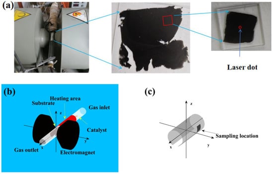
Figure 1.
(a) Experimental device and sampling process. (b) Schematic diagram of experimental device. (c) Schematic diagram of sampling location.
The morphologies of the samples (see Appendix A) were characterized using a scanning electron microscope (SEM) (S-4800, Hitachi, Tokyo, Japan). The Raman spectra of the samples were obtained under a He-Ne laser (LabRAM HR Evolution, Hubei Nuclear Solid Physics Key Laboratory at Wuhan University, Wuhan, China) at 633 nm excitation through a 100× objective with a power of 1.9 mW.
3. Results
3.1. Characterization
Figure 2 illustrates the Raman spectra of the SWCNTs films. The characteristic peaks of SWCNTs generally fall into two categories. Radial breathing mode (RBM) signals appear in the range of 100 cm−1 to 350 cm−1, and their frequencies are inversely proportional to the diameter of the SWCNTs () [17]. For the Raman spectra with a laser wavelength of 633 nm, the RBM peaks of s-SWCNTs are in the range of 120–180 cm−1, and the RBM peaks of m-SWCNTs are in the range of 180–240 cm−1 [18]. High-energy mode (HEM) signals occur in the range of 1500 cm−1 to 1650 cm−1, known as G peaks. The G peaks of SWCNTs usually split into two peaks, i.e., the low frequency as peaks and the high frequency as peaks. The D peaks () are related to the defects. The SWCNTs films, synthesized at 1 T and 1223 K, 0.8 T and 1323 K, and 1.0 T and 1323 K, have fewer defects.
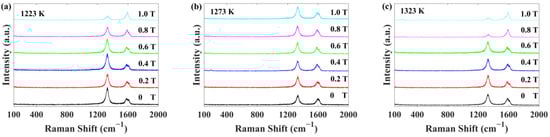
Figure 2.
Raman spectra of SWCNTs films synthesized under different temperatures and magnetic fields: (a) 1223 K, (b) 1273 K, and (c) 1323 K.
The G peaks of s-SWCNTs, corresponding to peaks, are Lorentz lines, and the G peaks of m-SWCNTs, corresponding to peaks, are BWF (Breit–Wigner–Fano) lines [19]. The fitting formula is as follows:
where is the intensity of the peak, is the peak frequency at the maximum intensity, is the full width at half maximum (FWHM) of the peak, is the intensity of the peak, is the peak frequency at the maximum intensity, is the FHWM of the peak, and is the measure of the interaction of the phonon with a continuum of states. As shown in Figure A2, Figure A3 and Figure A4 (see Figure A2, Figure A3 and Figure A4 in Appendix B), we fitted the G peaks with Formula (1). The fitting data are shown in Table 1. is the area of the peaks, and is the area of the peaks. Figure 3a illustrates the FHWM of the G peak. The FHWM of the G peaks widened as the defects increased. Figure 3b illustrates varying with the magnetic field. The of SWCNTs films synthesized at 1223 K has a peak at 0.8 T. The of SWCNTs films synthesized at 1273 K has two peaks at 0.4 T and 0.8 T. The of SWCNTs films synthesized at 1323 K has no peak.

Table 1.
Fitting data of G peaks.
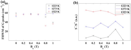
Figure 3.
(a) FHWM of G peaks of SWCNTs films synthesized under different temperatures and magnetic fields. (b) The curves of varying with the magnetic field.
The RBM peaks are Lorentz lines. As shown in Figure 4, we fitted the RBM peaks with the Formula (2):
where is the intensity of the RBM peak, is the RBM peak frequency at the maximum intensity, and is the FHWM of the RBM peak. The fitting data are shown in Table 2. is the area of the RBM peak. M-SWCNTs with the diameter of 1.28 nm and 1.24 nm were synthesized at 1273 K. m-SWCNTs with the diameter of 1.28 nm were synthesized at 1273 K. m-SWCNTs with the diameter of 1.24 nm and 1.14 nm were synthesized at 1323 K.
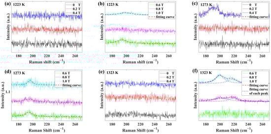
Figure 4.
RBM peaks of SWCNTs films synthesized at different conditions and the fitting curves. (a,b) 1223 K, (c,d) 1273 K, and (e,f) 1323 K.
Table 2.
Fitting data of RBM peaks.
3.2. Carrier Flow
It can be considered that the pressure () of the carrier flow was constant. We obtained Formula (3) by ignoring the gas reaction loss:
where is the flow rate at the gas inlet, is the temperature at the gas inlet, is the flow rate in the film-forming area, is the temperature in the film-forming area, is the average velocity of the carrier flow, and is the inner radius of the glass tube.
According to Formulas (3) and (4),
where , , , and ,
The Reynolds number () of the experimental system is as follows:
where is the diameter of the glass tube, is the kinematic viscosity of the carrier flow, , , and (the kinematic viscosity of Ar at 298 K),
It is generally considered that the flow is laminar with and the velocity distribution of laminar flow in the tube is parabolic [20]. The velocity distribution of the carrier flow () is shown as follows:
3.3. Magnetic Field
We assumed that the magnetic charge density on the surface was uniform. As shown in Figure 5a, the magnetic induction intensity () at point A, generated from the magnetic charge at points B and C, is as follows:
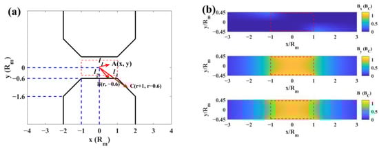
Figure 5.
(a) The xy-plane of the electromagnet. (b) The simulation of the magnetic induction intensity distribution. The film-forming area is in the red rectangle.
Due to the rotational and mirror symmetry of the magnetic field, the magnetic induction intensity is as follows:
where is the induction intensity along the x-direction and is the induction intensity along the y-direction. According to Formulas (11) and (12), the magnetic field distribution is shown in Figure 5b.
4. Discussion
4.1. Dynamic Analysis of m-SWCNTs Flow
In the film-forming area, SWCNTs were mainly affected by the magnetic force, drag force, viscous force, etc. Since [3,4,5], the magnetic force on the m-SWCNTs was considered, while the effect of the magnetic field on s-SWCNTs was ignored. The motion behavior of m-SWCNTs flow was analyzed below.
The m-SWCNTs lined up along the direction of the magnetic field as a result of the magnetic field [21]. The magnetic dipole () of m-SWCNTs is as follows:
where is the mass of m-SWCNTs and is the vacuum magnetic permeability.
The magnetic force () on a small magnet is as follows:
As shown in Figure 5, the magnetic field area coincided with the film-forming area and the direction of the magnetic field was almost parallel to the y-direction. According to Formulas (13) and (14),
where is the magnetic force along the x-direction and is the magnetic force along the y-direction. The distribution of was obtained using Formulas (11), (12) and (16) and is shown in Figure 6a. As shown in Figure 6b, was simplified to Formula (17):
where is the radius of the electromagnet.
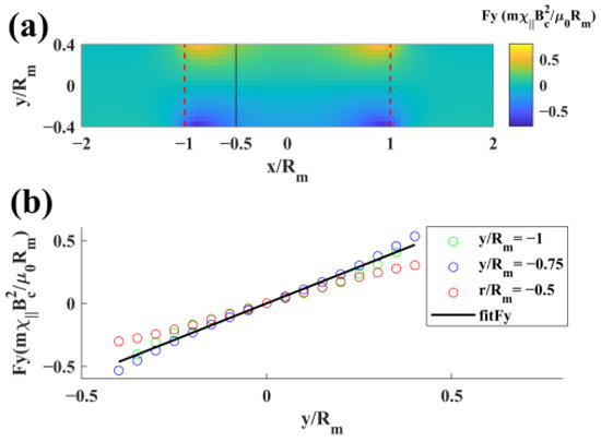
Figure 6.
(a) Simulation distribution of the magnetic force along the y-direction. (b) Linear fitting of the magnetic force distribution in the region from x = −Rm to x = −0.5Rm.
Due to the viscous force and its rod-like structure, we assumed that the velocity of the m-SWCNTs in the x-direction is equal to and ignored the viscous force in the y-direction. The motion equations of m-SWCNTs are as follows:
According to Formulas (9) and (17)–(23), the trajectory equation of m-SWCNTs is as follows:
4.2. Calculation of the Axial Magnetic Susceptibility
Assuming that m-SWCNTs were not produced in the film-forming area, we obtained Formulas (25) and (26):
where is the flux density of m-SWCNTs flow in the x-direction at , is the flux density of m-SWCNTs flow in the y-direction at , is the density of m-SWCNTs flow before entering the film-forming area, and is the velocity of m-SWCNTs flow at . Since the SWCNTs could not be synthesized near the tube wall [22], approached zero as approached .
According to Formulas (25) and (26),
As shown in Figure 3b and Figure 7, both the and of SWCNTs films synthesized at 1273 K have a peak at 0.4 T, indicating that the quantity of a type of m-SWCNTs () synthesized at 1273 K reached its maximum at 0.4 T. In contrast, the of SWCNTs films synthesized at 1223 K and 1323 K has no peak at 0.4 T, consistent with the finding that the Raman spectra (Figure 4) of these samples have no RBM peak similar to the m-SWCNTs (). The quantity of this type of m-SWCNTs is negligible at 1223 K and cannot be synthesized at 1323 K. It can be concluded that characterizes the quantity of a type of m-SWCNTs () at the sampling position, and characterizes the quantity of m-SWCNTs at the sampling position. is proportional to :
where is a constant. With the weak magnetic field, m-SWCNTs in the samples mainly came from the sites near the tube wall. is zero at 0 T and 0.2 T, indicating that this kind of m-SWCNTs could not be synthesized near the tube wall. To simplify the calculation, we took as a constant and fitted with Formulas (27)–(29), except for 0.2 T. The fitting curve is shown in Figure 7. The fitting result was as follows:
where , , , and ,
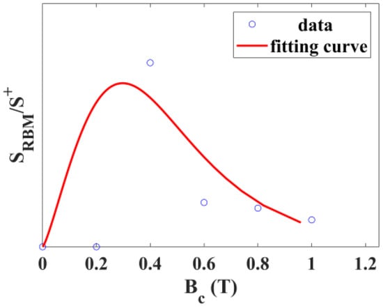
Figure 7.
Fitting curve of of SWCNTs films synthesized at 1273 K, varying with the central magnetic induction intensity.
The SWCNTs films synthesized at 1223 K and 1.0 T, 1323 K and 0.8 T, and 1323 K and 1.0 T had fewer defects. This phenomenon could be because m-SWCNTs with defects had high axial magnetic susceptibilities, were subject to high magnetic forces, and were deposited on the substrates before the sampling location.
This is the first time that the of m-SWCNTs has been measured. Previous studies on magnetic susceptibility and anisotropy are shown in Table 3. The of m-SWCNTs, without distinguishing and , is interpreted as follows:
where is a variable related to the arrangement of m-SWCNTs. It can be concluded that
Table 3.
The magnetic susceptibility (anisotropy) of SWCNTs.
According to Table 3, the magnitude of the of purified m-SWCNTs is not more than at 300 K. The of m-SWCNTs () with defects at 1273 K is at least two orders of magnitude greater than that of purified m-SWCNTs at 300 K. Combining the experimental results with the Curie–Weiss law, it can be concluded that the defects increase the Curie temperature and Curie constant of m-SWCNTs. The spin-polarized density functional theory predicts that m-SWCNTs with vacancies have local magnetic moments around the vacancies and exhibit ferro- or ferrimagnetism [7]. The experimental results are consistent with the spin-polarized density functional theory.
5. Conclusions
In a magnetic field-assisted FC-CVD, some SWCNTs films were synthesized under different magnetic fields and temperatures. The content of m-SWCNTs in the films varied with the magnetic field, and a model was built to describe this change by analyzing the motion behavior of m-SWCNTs flow in the field-assisted FC-CVD. The axial magnetic susceptibility of m-SWCNTs was obtained as a parameter in the model. The axial magnetic susceptibility of m-SWCNTs () with defects was at 1273 K. This is the first time that the axial magnetic susceptibility of m-SWCNTs has been obtained, and the result at 1273 K is at least two orders of magnitude greater than purified m-SWCNTs at 300 K. This difference is caused by the defects and conforms to the spin-polarized density functional theory, which predicts that m-SWCNTs with vacancies have local magnetic moments around the vacancies and exhibit ferro- or ferrimagnetism [7]. This study introduces a novel approach to investigating the magnetic properties of SWCNTs and provides the basis for the precise preparation of SWCNTs materials.
Author Contributions
Conceptualization, T.S. and C.P.; methodology, T.S.; software, T.S.; validation, T.S., Q.F. and C.P.; formal analysis, T.S.; investigation, T.S.; resources, Q.F. and C.P.; data curation, T.S.; writing—original draft preparation, T.S.; writing—review and editing, C.P.; visualization, T.S.; project administration, C.P.; funding acquisition, C.P. All authors have read and agreed to the published version of the manuscript.
Funding
This work was supported by the National Nature Science Foundation of China (no. 52272233, 11174227).
Institutional Review Board Statement
Not applicable.
Informed Consent Statement
Not applicable.
Data Availability Statement
The raw data supporting the conclusions of this article will be made available by the authors on request.
Acknowledgments
The Raman spectrometer (LabRAM HR Evolution) was provided by the Hubei Nuclear Solid Physics Key Laboratory at Wuhan University.
Conflicts of Interest
The authors declare no conflicts of interest.
Appendix A
As shown in Figure A1, SWCNTs films were synthesized under different conditions. SWCNTs formed networks at the mesoscopic scale and were surrounded by particles. With the adjustment of preparation conditions, the number of particles was almost constant, except at 1.0 T and 1273 K. This difference was caused by the different quality of SWCNTs films.
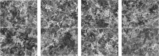
Figure A1.
SEM morphologies of SWCNTs films synthesized under different conditions: (a) 0 T and 1223 K, (b) 0 T and 1323 K, and (c–h) 0 T, 0.2 T, 0.4 T, 0.6 T, 0.8 T, and 1.0 T and 1273 K.
Appendix B
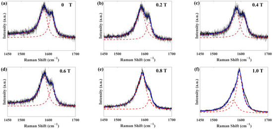
Figure A2.
G peaks of SWCNTs films synthesized at 1223 K under different magnetic fields. (a) 0 T, (b) 0.2 T, (c) 0.4 T, (d) 0.6 T, (e) 0.8 T, (f) 1.0 T. The black lines are Raman spectra of G peaks. The blue lines are the fitting curves of G peaks. The red lines are the fitting curves of and peaks.
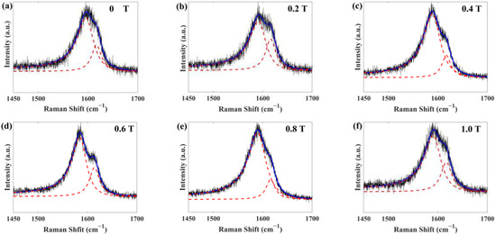
Figure A3.
G peaks of SWCNTs films synthesized at 1273 K under different magnetic fields (a) 0 T, (b) 0.2 T, (c) 0.4 T, (d) 0.6 T, (e) 0.8 T, (f) 1.0 T. The black lines are Raman spectra of G peaks. The blue lines are the fitting curves of G peaks. The red lines are the fitting curves of and peaks.
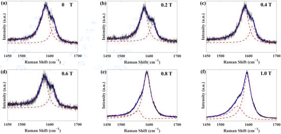
Figure A4.
G peaks of SWCNTs films synthesized at 1323 K under different magnetic fields. (a) 0 T, (b) 0.2 T, (c) 0.4 T, (d) 0.6 T, (e) 0.8 T, (f) 1.0 T. The black lines are Raman spectra of G peaks. The blue lines are the fitting curves of G peaks. The red lines are the fitting curves of and peaks.
References
- Iijima, S. Helical microtubules of graphitic carbon. Nature 1991, 354, 56–58. [Google Scholar] [CrossRef]
- Saito, R.; Fujita, M.; Dresselhaus, G.; Dresselhaus, M.S. Electronic structure of chiral graphene tubules. Appl. Phys. Lett. 1992, 60, 2204–2206. [Google Scholar] [CrossRef]
- Jianping, L. Novel Magnetic Properties of carbon nanotube. Phys. Rev. Lett. 1995, 74, 1123–1126. [Google Scholar] [CrossRef] [PubMed]
- Ajiki, H.; Ando, T. Magnetic properties of carbon nanotubes. J. Phys. Soc. Jpn. 1993, 62, 2470–2480. [Google Scholar] [CrossRef]
- Ajiki, H.; Ando, T. Magnetic properties of ensembles of carbon nanotubes. J. Phys. Soc. Jpn. 1995, 64, 4382–4391. [Google Scholar] [CrossRef]
- Marques, M.A.L.; d’Avezac, M.; Mauri, F. Magnetic response and NMR spectra of carbon nanotubes from ab initio calculations. Phys. Rev. B 2006, 73, 125433. [Google Scholar] [CrossRef]
- Ma, Y.C.; Lehtinen, P.O.; Foster, A.S.; Nieminen, R.M. Magnetic properties of vacancies in graphene and single-walled carbon nanotubes. New J. Phys. 2004, 6, 68. [Google Scholar] [CrossRef]
- Zaric, S.; Ostojic, G.N.; Kono, J.; Shaver, J.; Moore, V.C.; Strano, M.S.; Hauge, R.H.; Smalley, R.E.; Wei, X. Optical signatures of the Aharonov-Bohm phase in single-walled carbon nanotubes. Science 2004, 304, 1129–1131. [Google Scholar] [CrossRef] [PubMed]
- Islam, M.F.; Milkie, D.E.; Torrens, O.N.; Yodh, A.G.; Kikkawa, J.M. Magnetic heterogeneity and alignment of single wall carbon nanotubes. Phys. Rev. B 2005, 71, 201401. [Google Scholar] [CrossRef]
- Torrens, O.N.; Milkie, D.E.; Ban, B.Y.; Zheng, M.; Onoa, G.B.; Gierke, T.D.; Kikkawa, J.M. Measurement of chiral-dependent magnetic anisotropy in carbon nanotubes. J. Am. Chem. Soc. 2007, 129, 252–253. [Google Scholar] [CrossRef]
- Searle, T.A.; Imanaka, Y.; Takamasu, T.; Ajiki, H.; Fagan, J.A.; Hobbie, E.K.; Kono, J. Large anisotropy in the magnetic susceptibility of metallic carbon nanotubes. Phys. Rev. Lett. 2010, 105, 017403. [Google Scholar] [CrossRef]
- Kim, Y.H.; Torrens, O.N.; Kikkawa, J.M.; Abou-Hamad, E.; Goze-Bac, C.; Luzzi, D.E. High-purity diamagnetic single-wall carbon nanotube buckypaper. Chem. Mater. 2007, 19, 2982–2986. [Google Scholar] [CrossRef]
- Chuxin, W.; Jiaxin, L.; Guofa, D.; Lunhui, G. Removal of ferromagnetic metals for the large-scale purification of single-walled carbon nanotubes. J. Phys. Chem. C 2009, 113, 3612–3616. [Google Scholar] [CrossRef]
- Zaka, M.; Ito, Y.; Wang, H.L.; Yan, W.J.; Robertson, A.; Wu, Y.M.A.; Rümmeli, M.H.; Staunton, D.; Hashimoto, T.; Morton, J.J.L.; et al. Electron Paramagnetic resonance investigation of purified catalyst-free single-walled carbon nanotube. ACS Nano 2010, 4, 7708–7716. [Google Scholar] [CrossRef] [PubMed]
- Nakai, Y.; Tsukada, R.; Miyata, Y.; Saito, T.; Hata, K.; Maniwa, Y. Observation of the intrinsic magnetic susceptibility of highly purified single-wall carbon nanotubes. Phys. Rev. B 2015, 92, 041402. [Google Scholar] [CrossRef]
- Chengzhi, L.; Da, W.; Junji, J.; Delong, L.; Chunxu, P.; Lei, L. A rational design for the separation of metallic and semiconducting single-walled carbon nanotubes using a magnetic field. Nanoscale 2016, 8, 13017–13024. [Google Scholar] [CrossRef] [PubMed]
- Jorio, A.; Saito, R.; Hafner, J.H.; Lieber, C.M.; Hunter, M.; McClure, Y.; Dresselhaus, G.; Dresselhaus, M.S. Structural (n, m) determination of isolated single-wall carbon nanotubes by resonant raman scattering. Phys. Rev. Lett. 2001, 86, 1118–1121. [Google Scholar] [CrossRef]
- LeMieux, M.C.; Roberts, M.; Barman, S.; Jin, Y.M.; Kim, J.M.; Bao, Z.N. Self-sorted, aligned nanotube networks for thin-film transistors. Science 2008, 321, 101–104. [Google Scholar] [CrossRef] [PubMed]
- Brown, S.D.M.; Jorio, A.; Corio, P.; Dresselhaus, M.S.; Dresselhaus, G.; Saito, R.; Kneipp, K. Origin of the Breit-Wigner-Fano lineshape of the tangential G-band feature of metallic carbon nanotubes. Phys. Rev. B 2001, 63, 155414. [Google Scholar] [CrossRef]
- Pavelyev, A.A.; Reshmin, A.I.; Teplovodskii, S.K.; Fedoseev, S.G. On the lower critical Reynolds number for flow in a circular pipe. Fluid Dyn. 2003, 38, 545–551. [Google Scholar] [CrossRef]
- Wang, B.; Ma, Y.F.; Li, N.; Wu, Y.P.; Li, F.F.; Chen, Y.S. Facile and scalable fabrication of well-aligned and closely packed single-walled carbon nanotube films on various substrates. Adv. Mater. 2010, 22, 3067–3070. [Google Scholar] [CrossRef] [PubMed]
- Gspann, T.S.; Smail, F.R.; Windle, A.H. Spinning of carbon nanotube fibres using the floating catalyst high temperature route: Purity issues and the critical role of sulphur. Faraday Discuss. 2014, 173, 47–65. [Google Scholar] [CrossRef] [PubMed]
Disclaimer/Publisher’s Note: The statements, opinions and data contained in all publications are solely those of the individual author(s) and contributor(s) and not of MDPI and/or the editor(s). MDPI and/or the editor(s) disclaim responsibility for any injury to people or property resulting from any ideas, methods, instructions or products referred to in the content. |
© 2024 by the authors. Licensee MDPI, Basel, Switzerland. This article is an open access article distributed under the terms and conditions of the Creative Commons Attribution (CC BY) license (https://creativecommons.org/licenses/by/4.0/).