The Flow Stress–Strain and Dynamic Recrystallization Kinetics Behavior of High-Grade Pipeline Steels

Abstract

The hot deformation behavior of high-grade pipeline steels was studied in the strain rate range of 0.001~0.1 s⁻¹ and the temperature range of 1050~1200 °C by using hot compression tests on a Gleeble 3500 thermomechanical simulator. The flow stress increases with the increase in strain rate and the decrease in deformation temperature, and the deformation activation energy is about 358 kJ/mol. The flows stress–strain behavior of the work-hardening and dynamic recovery (DRV) was calculated using the Estrin–Mecking equation, and the kinetics model of the dynamic recrystallization (DRX) was established based on the Avrami equation through characteristic strains. Furthermore, the flow stress–strain behavior of high-grade pipeline steels was predicted by the established model based on the coupling effects of DRV and DRX. The corresponding predicted results are in good agreement with the experimental results according to standard statistical parameters analysis. Finally, the economic strain (ε₃) is proposed by the third derivative of the given kinetic model. Based on these calculation results, when the economic strain (ε₃) is reached, uniform and refined DRX grains can be obtained, the energy consumption reduced, and the production costs controlled, which is of great significance to actual factory production.

1. Introduction

Due to the combination of high strength and toughness, high-grade pipeline steels, such as, X70, X80, and X100, has been extensively studied [1,2,3,4,5]. Thermo-mechanical control process (TMCP) is an indispensable and important technology in the manufacture of high-grade pipeline steels, which mainly involves the thermal deformation process of steel plates. During the thermal deformation process, the flow stress reflects the difficulty of deformation of the material, and also puts forward corresponding requirements for the equipment capability. Thus, the accurate description of the flow behavior under different deformation conditions is of great significance for the design of the pipeline steel manufacturing process (excellent product performance) and the selection of manufacturing equipment (less energy consumption). Usually, a constitutive equation is used to describe the flow behavior of materials, such as the Arrhenius equation being applied to nickel-based alloys [6,7,8], steels [9,10,11], Ti alloys [12,13], and Al alloys [14,15]. The Johnson–Cook equation is used for a wide range of strain rates (e.g., 10⁻⁴ up to 10⁴ s⁻¹ [16,17,18]). The above method is called the phenomenological constitutive equation based on mathematical function fitting methods, and lacks obvious physical meaning [12,18]. On the other hand, under the evaluation of microstructure and deformation mechanisms of the materials, the flow stress was predicted by the Kocks–Estrin equation through considering the evolution of dislocation density [19,20]. However, the Kocks–Estrin equation can only describe the work-hardening and dynamic recovery (DRV). Under high temperature, the flow stress of many metals tends to have obvious stress peaks, meaning that the deformation mechanism is dominated by dynamic recrystallization, rather than a DRV. Generally, DRX consists of the process of nucleation and the grain boundary mobility, which can be described using the Avrami equation [21]. For example, the DRX kinetic behavior of a low-carbon steel during the hot deformation was studied using the Avrami model [22], where the volume fraction of DRX was predicted accurately. Based on the Avrami equation, the effect of the hot deformation parameters on the DRX behavior of X70 pipeline steel was studied and the evolution of volume fraction of DRX was described as a function of the different temperatures and strain rates [5]. A DRX kinetic model of the low-alloyed and micro-alloyed steels was proposed by Hernandez [23,24], and the flow stress–strain curve can also be predicted through the improved Avrami equation. This shows that the DRX behavior of pipeline steel can be accurately described using the Avrami equation. However, the establishment of a DRX kinetic model is only to predict the volume fraction of DRX. The evolution of the transform velocity of DRX is not analyzed in depth, and more useful information for the preparation process of pipeline steel cannot be obtained.

In this paper, X70 pipeline steel is the subject of research and the constitutive relationship between the flow stress and deformation parameters is established. The characteristic strains/stresses are obtained by the work-hardening rate curve. The volume fraction of DRX is obtained by the difference between the constructed flow stress curves of DRV and the experimental stress–strain curve. Then, the kinetic model is established based on the Avrami equation. The flow stress of X70 pipeline steel under different deformation conditions can be predicted by considering the coupling between the work-hardening behavior and the dynamic softening behavior of DRV and DRX. Finally, the economic strain (ε₃) is proposed by the third derivative of the given kinetic model of DRX for guaranteeing uniform and fine grains, saving energy consumption, and reducing production cost.

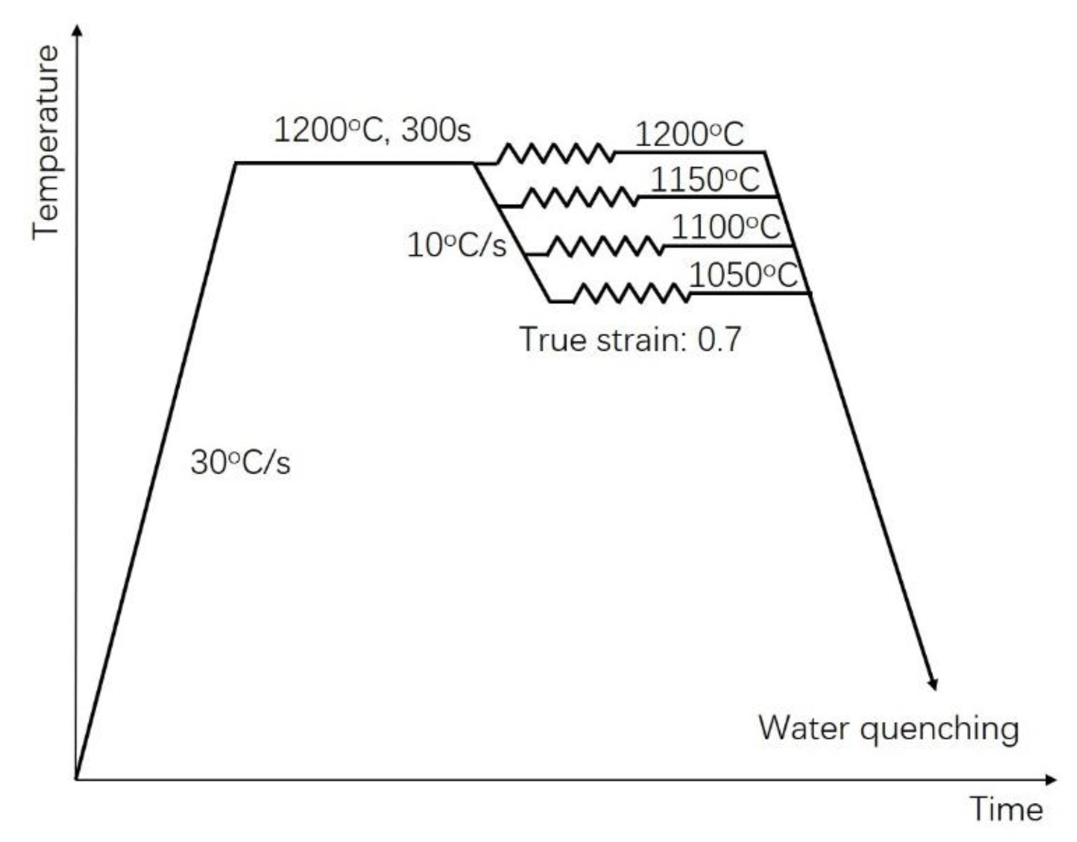
2. Materials and Methods

The chemical composition (wt%) of the X70 pipeline steel used in this work was as follows: C 0.05, Si 0.16, Mn 1.75, P 0.008, S 0.0024, Ni 0.1, Nb 0.053, V 0.0051, Cu 0.03, Ti 0.015. Before isothermal constant strain rate compression tests carried out on a Gleeble 3500 thermomechanical simulator were performed, all the specimens were heated to 1200 °C, held for 1 h, and then quenched to room temperature. The compression specimens were machined to a diameter of 10 mm and a length of 15 mm. To minimize the friction during hot deformation, tantalum foils were applied between the compression specimens and the platens. The compression specimens were heated to 1200 °C at a rate of 30 °C/s, holding for 300 s, then cooled to different deformation temperatures (1050~1150 °C) at a rate of 10 °C/s. All specimens were compressed to a true strain 0.7, then immediately water-cooled down to room temperature. The thermomechanical processing schedule is schematically shown in Figure 1.

Figure 1. Schematic diagram of thermomechanical processing schedule.

3. Results

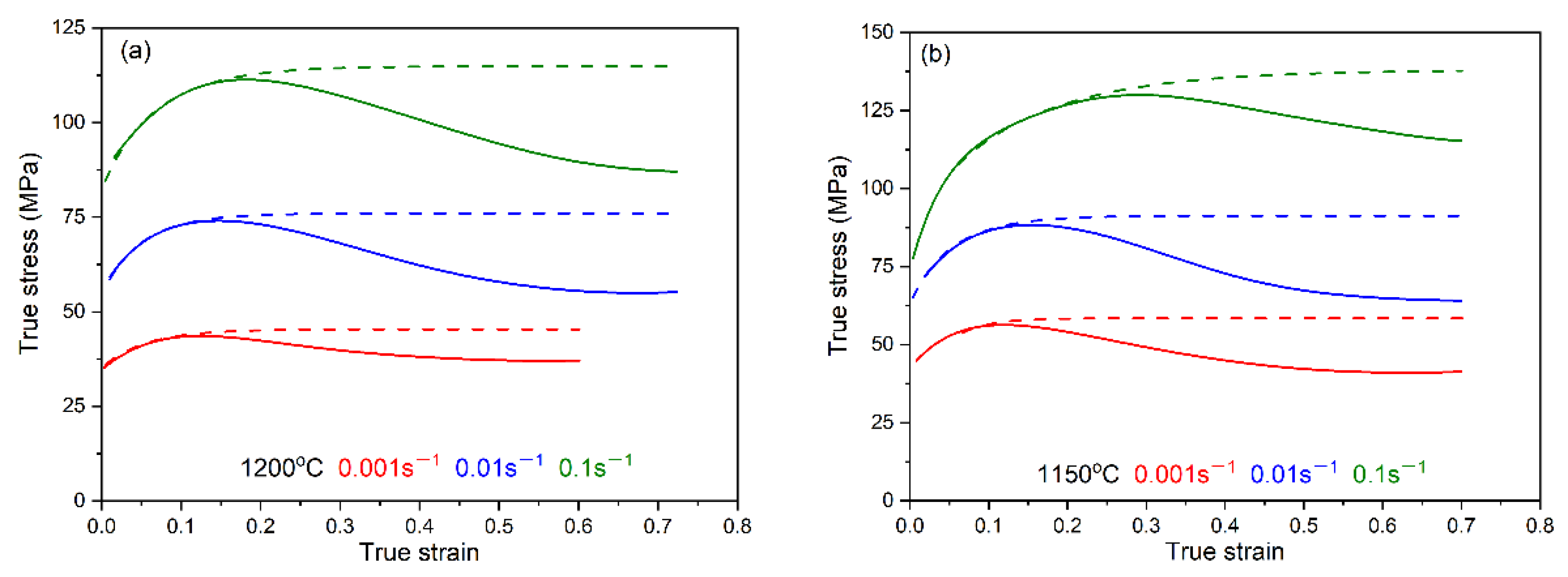
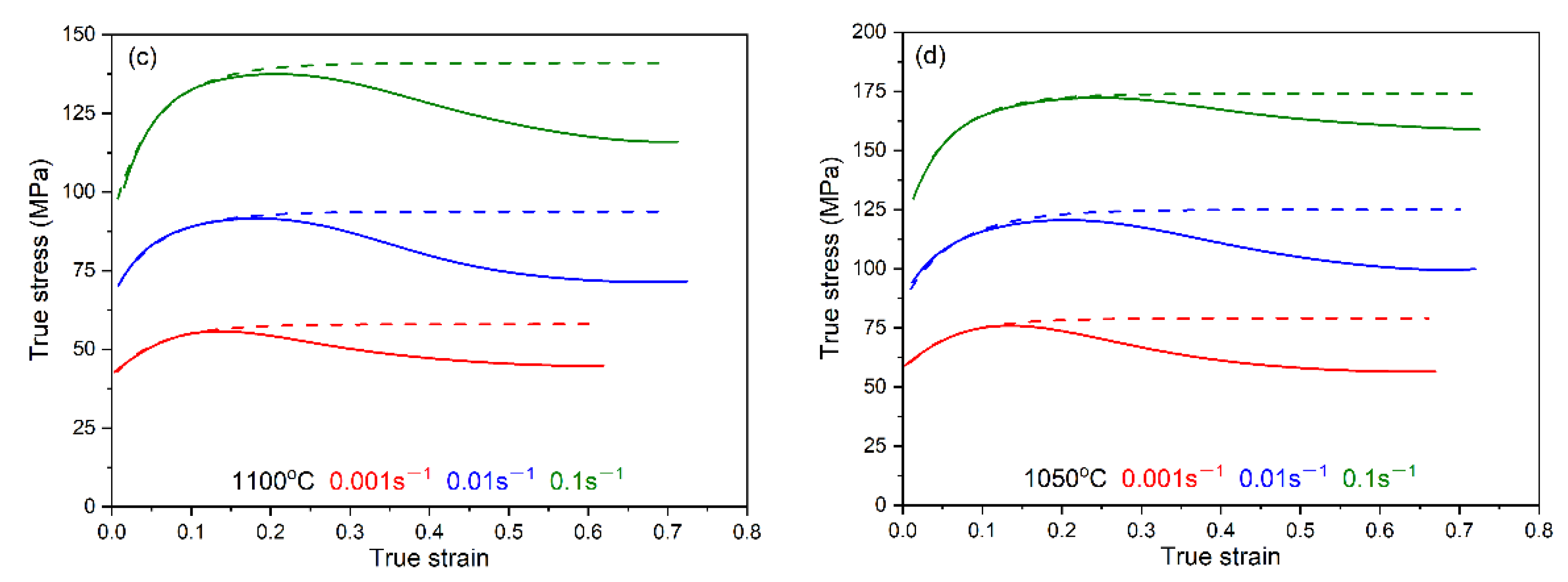
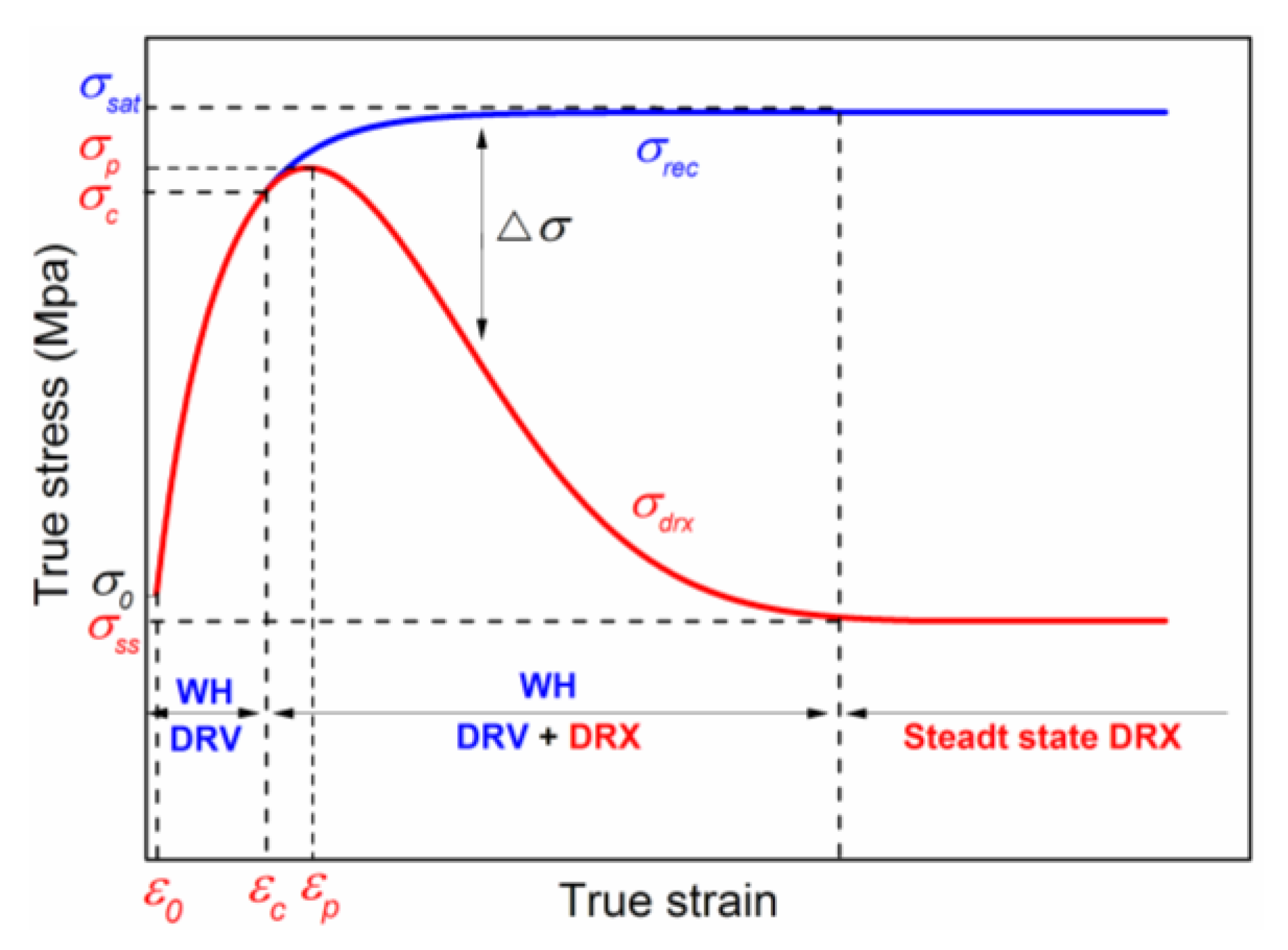
3.1. Flow Stress Curves

The flow stress–strain curves of the X70 pipeline steel at different deformation temperatures and strain rates in the isothermal compression tests are shown in Figure 2. During the hot deformation process, the shape of the flow stress curves is the result of competition between work-hardening and dynamic softening (DRV and DRX). As shown in Figure 2, at the initial stage of deformation, the flow stress increases rapidly due to the strong work-hardening behavior, based on the dislocation density, increases rapidly with small strain. When the critical strain is reached, the flow stress increases very slowly due to the occurrence of DRX softening, in which the nucleation process of DRX can consume a large number of dislocations. As the strain continue to increase, the flow stress peak occurs when the work-hardening is equal to the DRX softening. Thereafter, dynamic softening is greater than the work-hardening, and the flow stress gradually decreases until steady-state stress is reached. It can be found that the flow stress curve drops with the increase in temperature and with the decrease in the strain rate [25]. It is mainly because hot deformation is a thermally activated process. High temperature and low strain rate can promote the thermally activated process, reduce the critical stress for crystal grain slip, and enhance the recrystallized grain boundary migration, resulting in decreased work-hardening, as well as increased dynamic softening (DRV, DRX) [8,9,10,11].

Figure 2. Experimental flow stress–strain curves of the X70 pipeline steel under different strain rates of (a) 1200 °C, (b) 1150 °C, (c) 1100 °C, (d) 1050 °C.

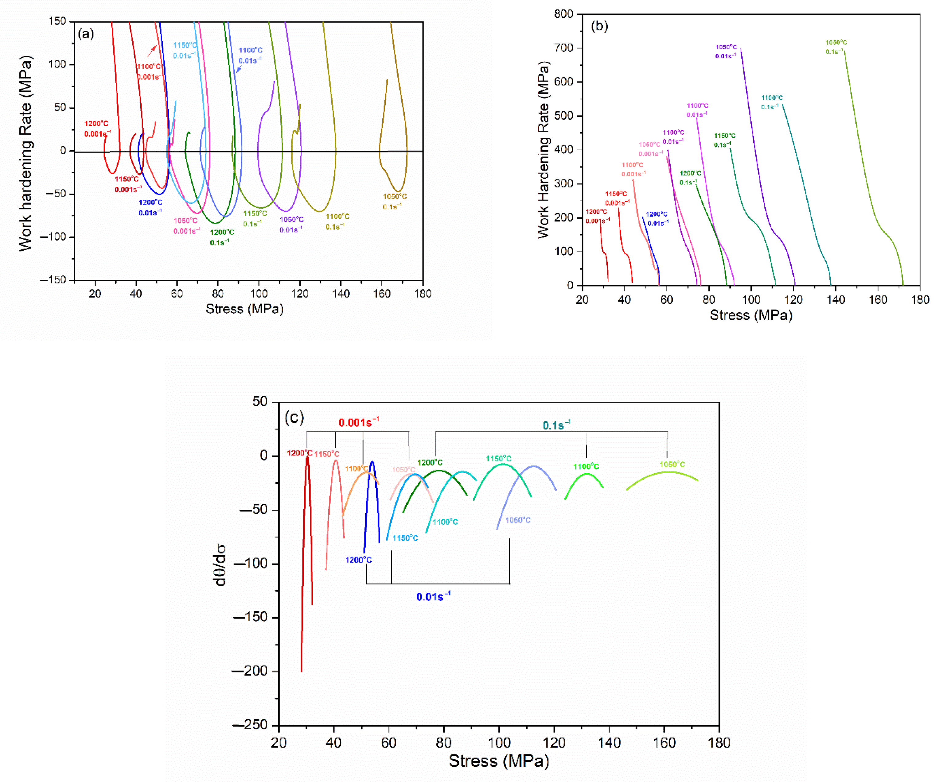
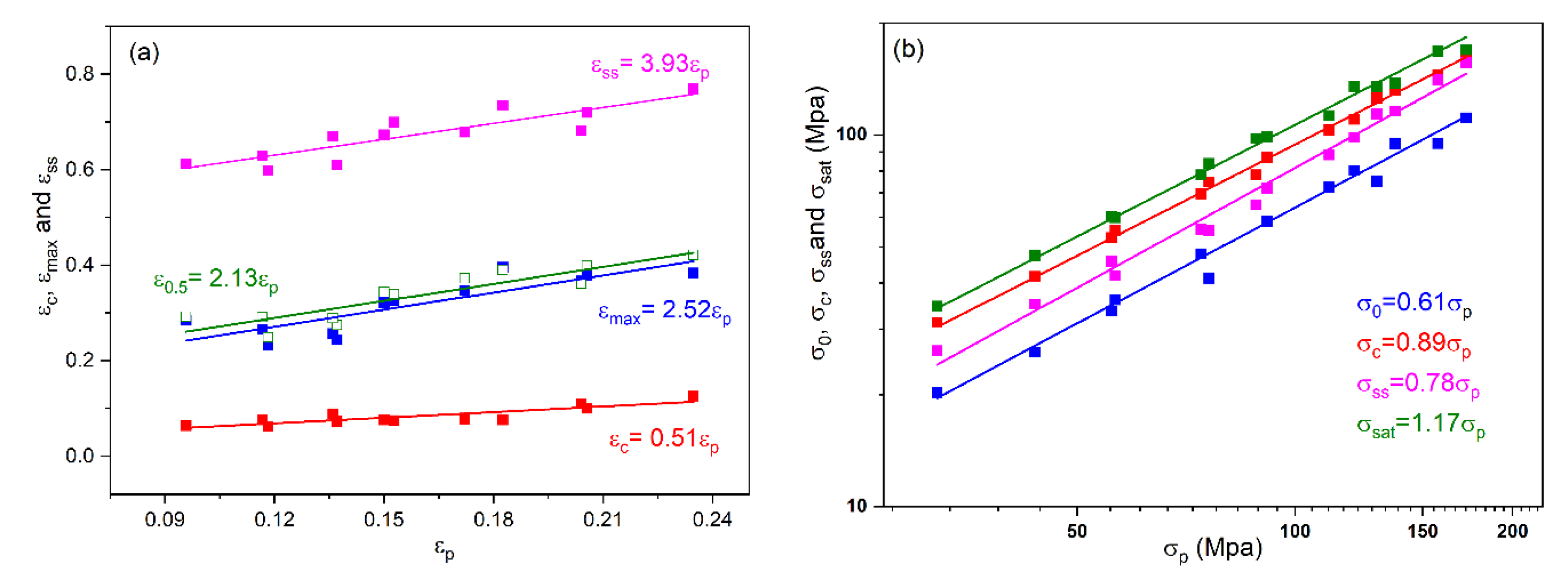
3.2. The Characteristic Stress/Strain

Usually, the characteristic stress of DRX softening curve can be obtained based on the working hardening rate (θ = dσ/dε) curve, including the critical stress (σ_c), the peak stress (σ_p), the maximum softening stress (σ_m), and the steady state stress (σ_ss) [22]. A typical total θ-σ curve of X70 pipeline steel is shown in Figure 3a, where, σ_p, σ_m, and σ_ss can be easily obtained. In order to determine the critical stress (σ_c) for the onset of DRX, Poliak and Jonas [26] proposed the double-differentiation method. Firstly, the local flow stress–strain curves from the yield stress (σ₀) to the peak stress (σ_p) were fitted using the seventh order polynomial. The working hardening rate curves under different deformation conditions are shown in Figure 3b. Then, when the derivative of the work-hardening rate curve is equal to 0, the critical stress (σ_c) is obtained under different deformation conditions, as shown in Figure 3c. All characteristic strains of DRX can be obtained from corresponding characteristic stresses in the flow stress curve.

Figure 3. The relationship between work-hardening rate and true stress of X70 pipeline steel in different deformation conditions: (a) whole curve; (b) local curve from yield to peak stress stage; (c) the second derivative of the work-hardening rate curve.

Since the peak stress/strain can be directly and accurately obtained from the experimental flow stress curve, the empirical relationship between the peak stress/strain and other characteristic stress/strain is often established. It can be seen from Figure 4a that the yield strain/stress, the critical stress/strain, the maximum softening stress/strain, and the steady state stress/strain show a good linear relationship with the peak strain, in which their empirical relationship can simply expressed as: ε_c = 0.51ε_p, ε_max = 2.52ε_p, and ε_ss = 3.93ε_p. Similarly, characteristic stresses are in a certain proportion to the peak stress (Figure 4b), which can be expressed as: σ_c = 0.89σ_p, σ₀ = 0.61σ_p, σ_ss = 0.78σ_p, and σ_sat = 1.17σ_p, respectively.

Figure 4. Relationship between characteristic parameter (strain (a) and stress (b)) and Z.

To establish the relationship between characteristic stresses/strains and processing parameters (deformation temperatures and strain rates), the constitutive equation can be used and expressed as follows:

$$\dot{\epsilon }=A_1{\sigma }_p^{m^{\ast }}\exp \left(-\frac{Q_d}{RT}\right)$$

(1)

$$\dot{\epsilon }=A_2\exp \left(\beta {\sigma }_p\right)\exp \left(-\frac{Q_d}{RT}\right)$$

(2)

$$\dot{\epsilon }=A{\left[\sinh \left(\alpha {\sigma }_p\right)\right]}^m\exp \left(-\frac{Q_d}{RT}\right)$$

(3)

Usually, the relationship between the deformation temperature and strain rate can be established through Zener–Hollomon parameter (Z) as follows [27]:

$$Z=\dot{\epsilon }\exp \left(\frac{Q_d}{RT}\right)=A{\left[\sinh \left(\alpha {\sigma }_p\right)\right]}^m$$

(4)

In Equations (1)–(4), Q_d is the deformation activation energy, R is the gas constant (8.314 Jmol⁻¹K⁻¹), and A, A₁, A₂, β, α, m, m* are the material constants. Firstly, the value of α in Equation (3) should be calculated as 0.0124 by using the relationship between β and m* (β/m*), where the average value of β and m* can be calculated as 0.07 and 5.39 by linear fitting, respectively. Then, the deformation activation energy (Q_d) can be obtained by partial differentiation of Equation (3):

$$Q_d=R{\left[\frac{\partial \dot{\ln \epsilon }}{\partial \ln \left(\sinh \left(\alpha {\sigma }_p\right)\right)}\right]}_T{\left[\frac{\partial \ln \left(\sinh \left(\alpha {\sigma }_p\right)\right)}{\partial \left(1/T\right)}\right]}_{\dot{\epsilon }}=RmS$$

(5)

The values of m can be obtained as 4.73 by calculating the average value of slopes under different deformation temperatures in Figure 5a, and the value of Q_d can be derived as 358 KJ/mol by calculating the average value of slops under different strain rates in Figure 5b. Finally, the constitutive equation of the X70 pipeline steel can be expressed as following:

$$\dot{\epsilon }=1.8123\times {10}^{16}{\left[\sinh 0.0124\right]}^{4.73}\exp \left(-\frac{358,656}{RT}\right)$$

(6)

Furthermore, the peak stress can be calculated by using Equation (7).

$${\sigma }_p=123.153\times \ln \left\{{\left[\frac{Z}{1.8123\times {10}^{16}}\right]}^{1/4.73}+{\left[{\left(\frac{Z}{1.8123\times {10}^{16}}\right)}^{2/4.73}+1\right]}^{1/2}\right\}$$

(7)

Figure 5. Relationship of ln[sinh(ασ_p)] vs. ln$\dot{\epsilon }$ (a); ln[sinh(ασ_p)] vs. 1/T (b) and the peak stress vs. Z (c) deduced from the X70 pipeline steel subjected to different deformation conditions.

Furthermore, based on the exponential relationship in Equation (7), a relatively simple exponential relationship between characteristic stresses/strains and Z parameter can be directly obtained, which is expressed as follows:

$${\mathsf{\sigma }}_{\mathrm{p}}=a{Z}^b {\sigma }_x=A{\mathsf{\sigma }}_{\mathrm{p}}=A\ast a{Z}^b$$

(8)

$${\mathsf{\epsilon }}_{\mathrm{p}}=c{Z}^d {\epsilon }_x=C{\mathsf{\epsilon }}_{\mathrm{p}}=C\ast c{Z}^d$$

(9)

where a, b, c and d are the material constants. The function relation between the peak stress/strain (σ_p/ε_p) and Z parameter can be obtained through linear regression. Furthermore, the relationship between other characteristic stresses and Z can also be determined one by one by using the above proportional relation (Equations (8) and (9)). The calculated results of the function relation are in Table 1.

Table 1. The relationship between characteristic stresses/strains and Z.

${\mathit{\sigma }}_{\mathit{x}}=\mathit{a}{\mathit{Z}}^{\mathit{b}}$	${\mathit{\epsilon }}_{\mathit{x}}=\mathit{c}{\mathit{Z}}^{\mathit{d}}$
σp = 0.993 × Z0.218	εp = 0.0085 × Z0.118
σc = 0.884 × Z0.218	εc = 0.00434 × Z0.118
σss = 0.775 × Z0.218	εss = 0.6091 × Z0.118
σsat = 1.162 × Z0.218	εm = 0.0214 × Z0.118
σ0 = 0.606 × Z0.218	ε0.5 = 0.181 × Z0.118

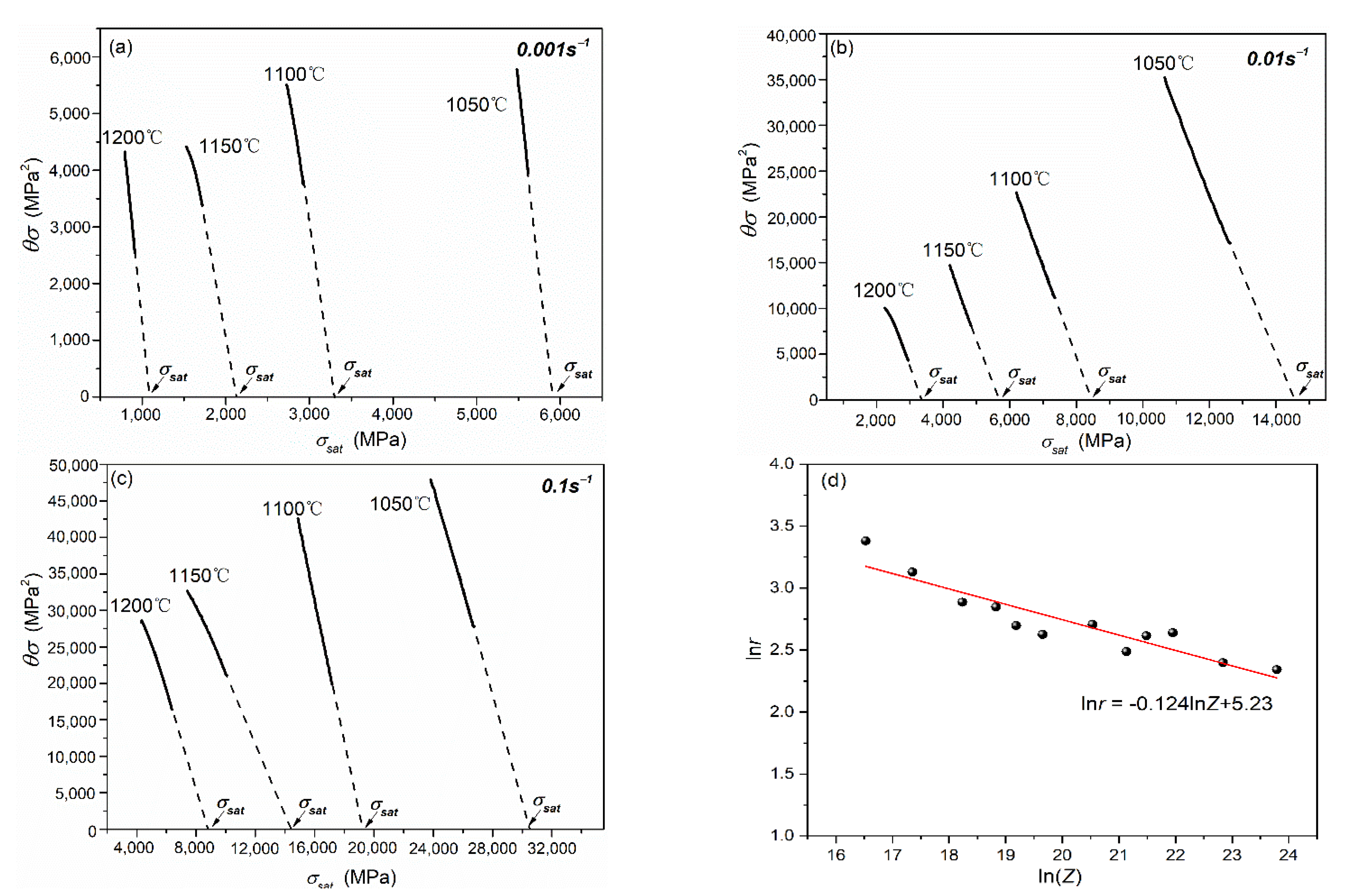
3.3. The Flow Behavior in DRV

The flow stress curve of DRV regime during hot deformation can be described by the competition between storage and annihilation process of dislocation. It can be expressed as follows [22,28]:

$$\frac{\mathrm{d}\mathsf{\rho }}{\mathrm{d}\mathsf{\epsilon }}=\mathrm{h}-\mathrm{rp}$$

(10)

where the first term on the right-hand side of Equation (10) represents the contribution of the work-hardening and the second term due to DRV. The work-hardening term can be regarded as constant (h) with respect to the strain; meanwhile, a parameter (r) of DRV follows the first order kinetics. When the initial dislocation density is denoted by $\mathsf{\rho }$₀, the evolution of dislocation density in the wok-hardening and DRV regime can be described by integrating Equation (10):

$$\mathsf{\rho }={\mathsf{\rho }}_0\exp \left(-\mathrm{r}\left(\mathsf{\epsilon }-{\mathsf{\epsilon }}_{\mathrm{o}}\right)\right)+\frac{\mathrm{h}}{\mathrm{r}}\left(1-\exp \left(-\mathrm{r}\left(\mathsf{\epsilon }-{\mathsf{\epsilon }}_0\right)\right)\right)$$

(11)

The relationship between the flow stress and the dislocation density is usually expressed as:

$$\mathsf{\sigma }=\mathsf{\alpha }\mathsf{\mu }\mathrm{b}\sqrt{\mathsf{\rho }}$$

(12)

where α is a material constant, μ is the shear modulus, and b is the magnitude of Burger’s vector. The value of the flow stress of DRV can be calculated by combining Equations (11) and (12), and is expressed as follows:

$${\mathsf{\sigma }}_{\mathrm{rec}}={\left({\mathsf{\sigma }}_0^2\exp \left(-\mathrm{r}\left(\mathsf{\epsilon }-{\mathsf{\epsilon }}_0\right)\right)+{\left(\mathsf{\alpha }\mathsf{\mu }\mathrm{b}\right)}^2\left(\frac{\mathrm{h}}{\mathrm{r}}\right)\left(1-\exp \left(-\mathrm{r}\left(\mathsf{\epsilon }-{\mathsf{\epsilon }}_0\right)\right)\right)\right)}^{\frac{1}{2}}$$

(13)

where σ_rec represents the flow stress of DRV, σ₀ the yield stress, and ε₀ the strain corresponding to σ₀. The relationship between the stress and the strain under DRV duration can be described as Equation (13). With the increase in the strain (ε), the stress (σ_rec) tends toward a saturation value (σ_sat) corresponding to an equilibrium between dislocation storage and dislocation annihilation, i.e., d$\mathsf{\rho }$/dε = 0, ${\mathsf{\sigma }}_{\mathrm{rec}}=\mathsf{\alpha }\mathsf{\mu }\mathrm{b}\sqrt{\mathrm{h}/\mathrm{r}}$. After the saturated stress (σ_sat) is brought into Equation (13), it can be expressed as the following formula:

$${\mathsf{\sigma }}_{\mathrm{rec}}={\left({\mathsf{\sigma }}_{\mathrm{sat}}^2-\left({\mathsf{\sigma }}_{\mathrm{sat}}^2-{\mathsf{\sigma }}_0^2\right)\exp \left(-\mathrm{r}\left(\mathsf{\epsilon }-{\mathsf{\epsilon }}_0\right)\right)\right)}^{\frac{1}{2}}$$

(14)

All the stress/strain parameters in Equation (14) were obtained in Section 3.2, so, as long as the r parameter is determined, the flow stress–strain curve of DRV can be obtained. The parameter r can be determined based on the differentiation of Equation (14) with respect to ε, and multiplication by σ_rec leads to the following relation [29]:

$$\frac{{\mathrm{d}\mathsf{\sigma }}_{\mathrm{rec}}}{\mathrm{d}\mathsf{\epsilon }}{\mathsf{\sigma }}_{\mathrm{rec}}={\mathsf{\theta }\mathsf{\sigma }}_{\mathrm{rec}}=\frac{1}{2}{\mathrm{r}\mathsf{\sigma }}_{\mathrm{sat}}^2-\frac{1}{2}{\mathrm{r}\mathsf{\sigma }}_{\mathrm{rec}}^2$$

(15)

where θ is the work-hardening rate prior to the critical strain (ε_c). In order to obtain the value of parameter r, the calculation formula is proposed by deriving Equation (16) with respect to ${\mathsf{\sigma }}_{\mathrm{rec}}^2$:

$$\mathrm{K}=\frac{\mathrm{d}\left({\mathsf{\theta }\mathsf{\sigma }}_{\mathrm{rec}}\right)}{{\mathrm{d}\mathsf{\sigma }}_{\mathrm{rec}}^2}=-\frac{1}{2}\mathrm{r}$$

(16)

According to Equation (16), the value of parameter r under different deformation conditions can be calculated as −2K and is shown in Figure 6, in which solid line is calculated from the experimental flow stress curve prior to σ_c. Meanwhile, the saturation stress (σ_sat) can also be obtained by the intersection of the dashed line and the abscissa indicated by arrows in Figure 6a–c.

Figure 6. The plot of σ² vs. θσ of the X70 pipeline steel at different deformation conditions: 0.001 s⁻¹ (a); 0.01 s⁻¹ (b); 0.1 s⁻¹ (c); and the relationship between parameter r and Z parameter in the X70 pipeline steel (d).

A functional relationship between the parameter r and different deformation conditions (Z) is established and is shown in Figure 6d. The parameter r decreases with the increase in the Z parameter, indicating that the dynamic recovery process is more difficult with the decrease in deformation temperature or the increase in strain rate. This is consistent with the research results of Jonas et al. [22], indicating that the occurrence difficulty of dynamic recovery process increases with the increase in stress value.

Based on the above analysis, the flow stress–strain curve of DRV for X70 pipeline steels can be summarized as:

$$\left\{\begin{array}{c}{\epsilon }_0=0.00171Z^{0.118}\\ {\sigma }_0=0.606Z^{0.218}\\ {\sigma }_{sat}=1.162Z^{0.218}\\ r=186.233Z^{-0.124}\\ {\mathsf{\sigma }}_{\mathrm{rec}}={\left({\sigma }_{sat}^2-\left({\sigma }_{sat}^2-{\sigma }_0^2\right)\exp \left(-r\left(\epsilon -{\epsilon }_0\right)\right)\right)}^{\frac{1}{2}}\end{array}\right.$$

(17)

Figure 2a–c are the prediction results, and it can be seen that the calculated flow stress curve of DRV at all deformation conditions coincide well with the experimental flow stress–strain curves before the critical stress/strain. After the critical stress/strain, the flow stress of DRV keeps increasing until it reaches the saturation stress (σ_sat). On the whole, the flow stress–strain curve of DRV increases with the decrease in temperature or the increase in strain rate.

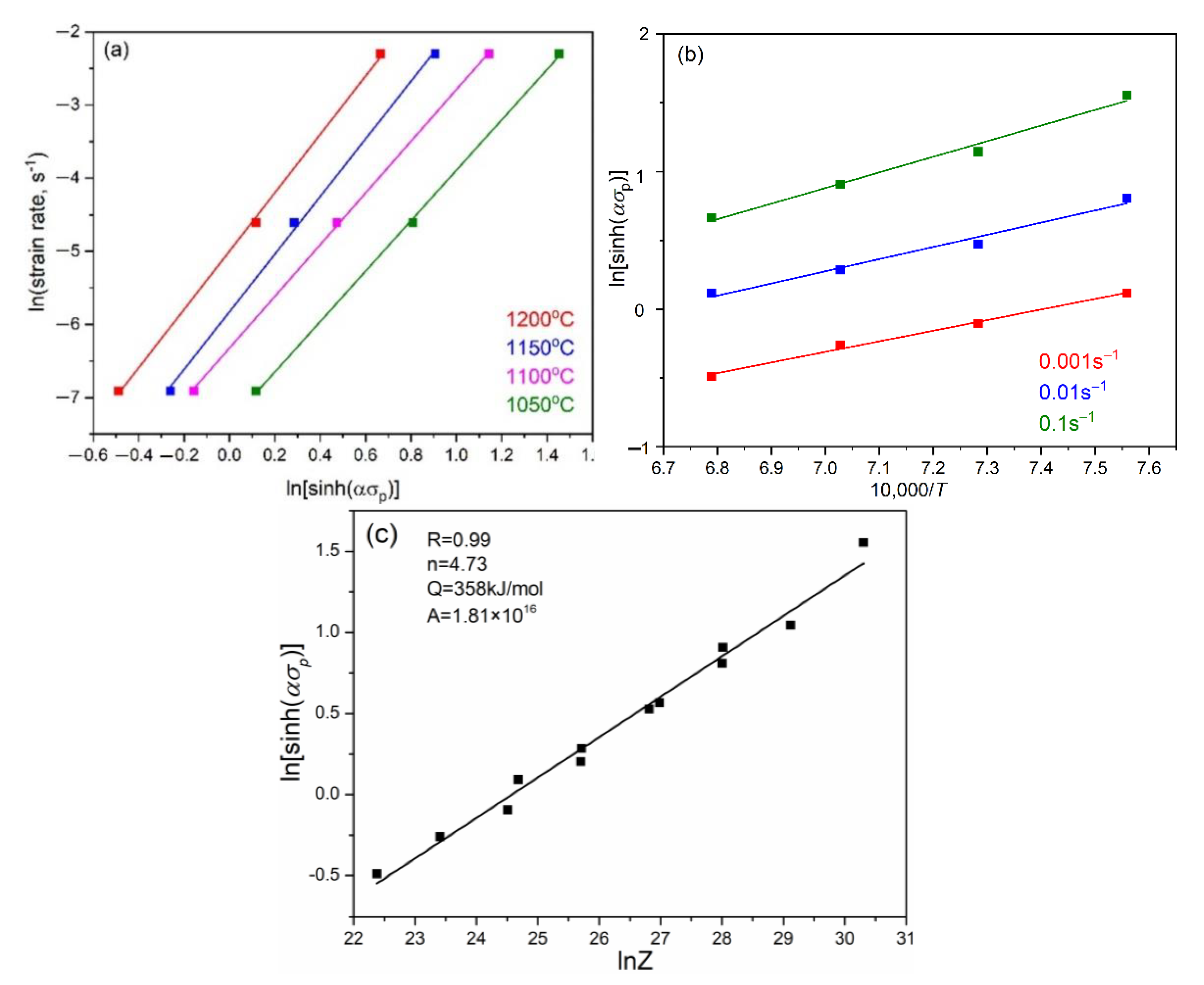
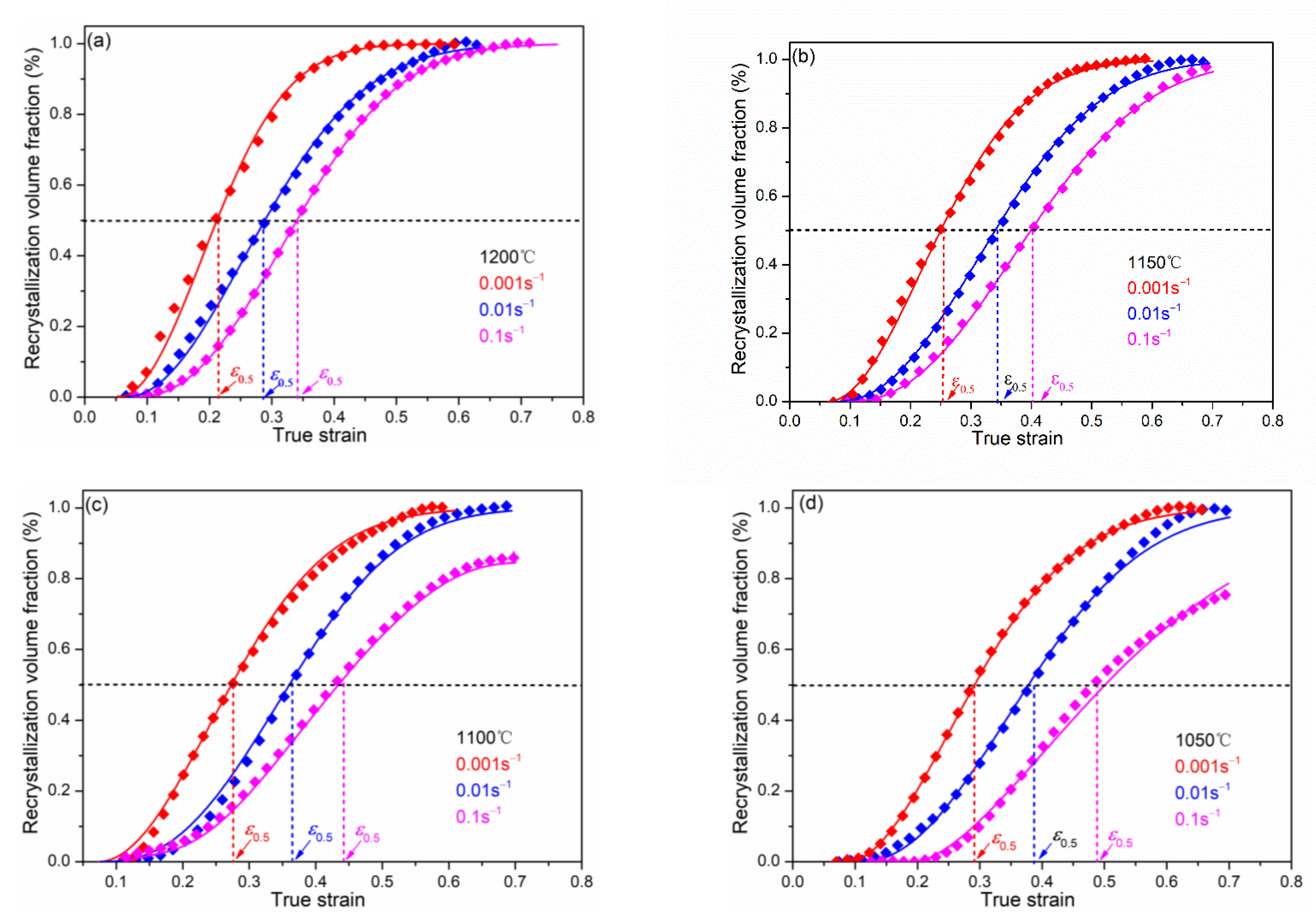
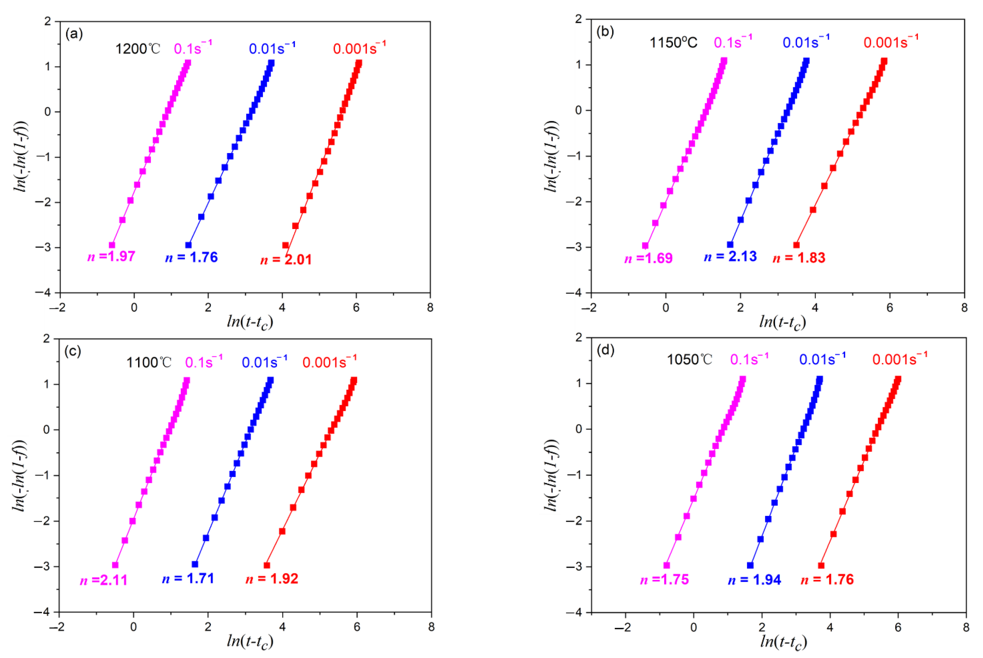
3.4. Kinetic Model of DRX

Figure 7 is a schematic diagram of the dynamic softening of flow stress at elevated temperature. After the critical stress, the flow stress presents two different characteristics represented by the “blue” and “read” lines in Figure 7, which are attributed to DRV and DRX, respectively. For the “blue” curve, when the work-hardening rate is equal to the DRV softening rate, the stress reaches saturation value and remains constant (σ_sat). For the “red” curve, after the flow stress reaches the peak stress, the DRX softening rate is stronger than the work-hardening rate resulting in the flow decreasing continuously to the steady state value (σ_ss). Therefore, using the difference between the experimental stress curve and the flow stress of DRV, the volume fraction of the DRX can be expressed as:

$$X_{DRX}=\frac{\Delta \sigma }{{\mathsf{\sigma }}_{\mathrm{sat}}-{\mathsf{\sigma }}_{\mathrm{ss}}}=\frac{{\mathsf{\sigma }}_{\mathrm{rec}}-{\mathsf{\sigma }}_{\mathrm{drx}}}{{\mathsf{\sigma }}_{\mathrm{sat}}-{\mathsf{\sigma }}_{\mathrm{ss}}}$$

(18)

Figure 7. Schematic diagram illustrates the work-hardening curve σ_rec (the red line) from yield stress σ₀ to saturation stress σ_sat in the entire strain domain, and a typical experimental DRX flow stress curve (the blue line) from yield stress σ₀ to steady state stress σ_ss.

According to Equation (19), the volume fraction of DRX at the different deformation conditions can be calculated easily, and this method is particularly useful for high-grade pipeline steels, where metallographic microstructures are difficult to carry out. As shown in Figure 8, with the increase in strain, the volume fraction of DRX firstly increases and then decreases, which shows a typical S-shaped curve.

Figure 8. Comparison between the experimentally (symbols) and predicted (solid curves) volume fraction of DRX: (a) 1200 °C, (b) 1150 °C, (c) 1100 °C, (d) 1050 °C.

When the critical strain (ε_c) is reached, the dislocation density near grain boundary is sufficient to promote the nucleation of DRX grains. With the increase in strain, DRX nucleation start to grow through the migration of new grain boundary. When the DRX transition is fully completed, the flow stress does not change with the increase in the strain, that is, the steady state stress occurs at this time. In this study, the volume fraction of DRX can be expressed generally as [29,30]:

$${\mathrm{X}}_{\mathrm{DRX}}=1-\exp \left(-0.693{\left(\frac{\mathsf{\epsilon }-{\mathsf{\epsilon }}_{\mathrm{c}}}{{\mathsf{\epsilon }}_{0.5}-{\mathsf{\epsilon }}_{\mathrm{c}}}\right)}^{\mathrm{n}}\right)$$

(19)

Taking logarithm of Equation (19) gives:

$$\ln \left(-\ln \left(1-{\mathrm{X}}_{\mathrm{DRX}}\right)\right)=\ln 0.693+\mathrm{nln}\left(\frac{\mathsf{\epsilon }-{\mathsf{\epsilon }}_{\mathrm{c}}}{{\mathsf{\epsilon }}_{0.5}-{\mathsf{\epsilon }}_{\mathrm{c}}}\right)$$

(20)

According to Equation (20), the average calculation result of n at all deformation conditions is 1.88, as shown in Figure 9, which is in consistent with the range of 1.3~2.5 observed by other works [22,24,29,30].

Figure 9. Value of Avrami index (n) at different deformation conditions. (a) 1200 °C; (b) 1150 °C; (c) 1100 °C; (d) 1050 °C.

Based on the above analysis, the kinetics equation of DRX for the X70 pipeline steel can be summarized as:

$$\left\{\begin{array}{c}{\mathsf{\epsilon }}_{\mathrm{c}}=0.000434{\mathrm{Z}}^{0.118}\\ {\mathsf{\epsilon }}_{0.5}=0.181{\mathrm{Z}}^{0.118}\\ {\mathrm{X}}_{\mathrm{DRX}}=1-\exp \left(-0.693{\left(\frac{\mathsf{\epsilon }-{\mathsf{\epsilon }}_{\mathrm{c}}}{{\mathsf{\epsilon }}_{0.5}-{\mathsf{\epsilon }}_{\mathrm{c}}}\right)}^{1.88}\right)\end{array}\right.$$

(21)

The comparison of the calculated and experimental result is shown in Figure 9. The calculated results are consistent with the experimental ones, indicating that the established kinetic equation can well-describe the DRX behavior of X70 pipeline steel during hot deformation process.

4. Application and Discussion

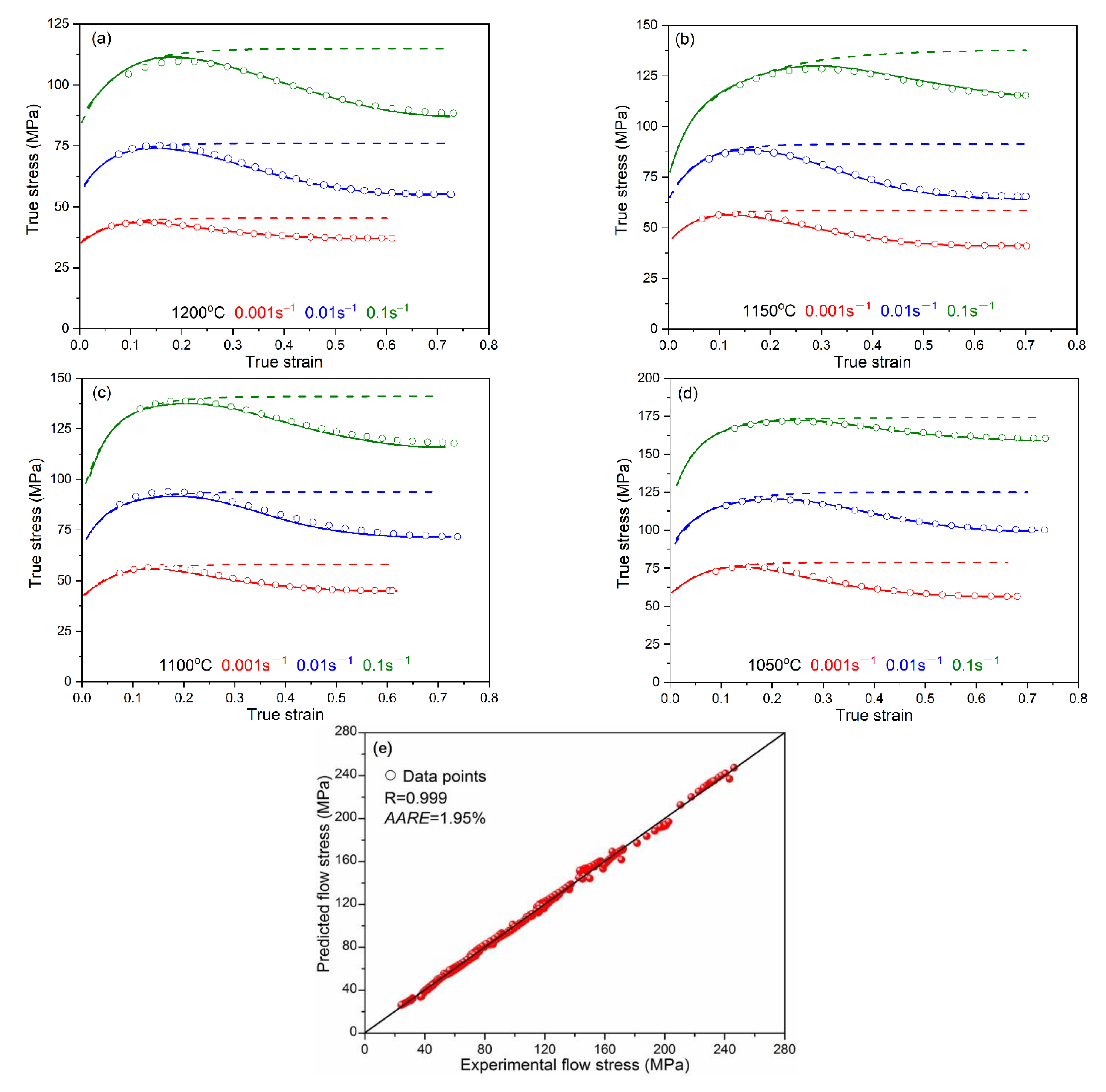
4.1. Prediction of Flow Stress Curves in DRV

The experimental flow stress curve can be predicted through incorporation between the DRV curve and DRX softening. By substituting Equations (19) and (21) into Equation (18), the flow stress–strain curve of high-grade pipeline steel can be obtained as follows:

$$\mathsf{\sigma }={\left({\mathsf{\sigma }}_{\mathrm{sat}}^2-\left({\mathsf{\sigma }}_{\mathrm{sat}}^2-{\mathsf{\sigma }}_0^2\right)\exp \left(-\mathrm{r}\left(\mathsf{\epsilon }-{\mathsf{\epsilon }}_0\right)\right)\right)}^{\frac{1}{2}}-\left({\mathsf{\sigma }}_{\mathrm{sat}}-{\mathsf{\sigma }}_{\mathrm{ss}}\right)\left(1-\exp \left(-0.693{\left(\frac{\mathsf{\epsilon }-{\mathsf{\epsilon }}_{\mathrm{c}}}{{\mathsf{\epsilon }}_{0.5}-{\mathsf{\epsilon }}_{\mathrm{c}}}\right)}^{1.88}\right)\right)$$

(22)

Comparison between the calculation and experimental results are shown in Figure 10, in which the scatter points and solid line represent the results of calculations and experiment results, respectively. It can be found that the calculated flow stress curves from Equation (22) are in good agreement with the experiment the flow curves. In order to quantitatively describe the prediction accuracy of the model, the correlation coefficient (R) and average absolute relative error (AARE) are used, and expressed as:

$$R=\frac{{{\displaystyle \sum }}_{i=1}^N\left(E_i-\overline{E}\right)\left(C_i-\overline{C}\right)}{\sqrt{{{\displaystyle \sum }}_{i=1}^N{\left(E_i-\overline{E}\right)}^2{{\displaystyle \sum }}_{i=1}^N{\left(C_i-\overline{C}\right)}^2}}$$

(23)

$$AARE\left(\%\right)=\frac{1}{N}{\displaystyle \sum }_{i=1}^N\left|\frac{E_i-C_i}{E_i}\right|\times 100\%$$

(24)

where E_i and C_i represents the experimental data and the calculated results, respectively. E and C are the mean values of E_i and C_i, respectively. N is the total number of data. The calculated result is shown as in Figure 10d, which shows a good correlation between the experimental and the calculated data through using Equation (22). The value of R and AARE for prediction equation are 0.999 and 1.95%, respectively. These results indicate that Equation (22) can predict accurately the flow stress-strain curve of the X70 pipeline steel.

Figure 10. Comparison between the predicted and experimental flow stress–strain curves from constitutive equation at strain rate (a) 1200 °C, (b) 1150 °C, (c) 1100 °C, (d) 1050 °C, (e) correlation between the experimental and predicted flow stress data.

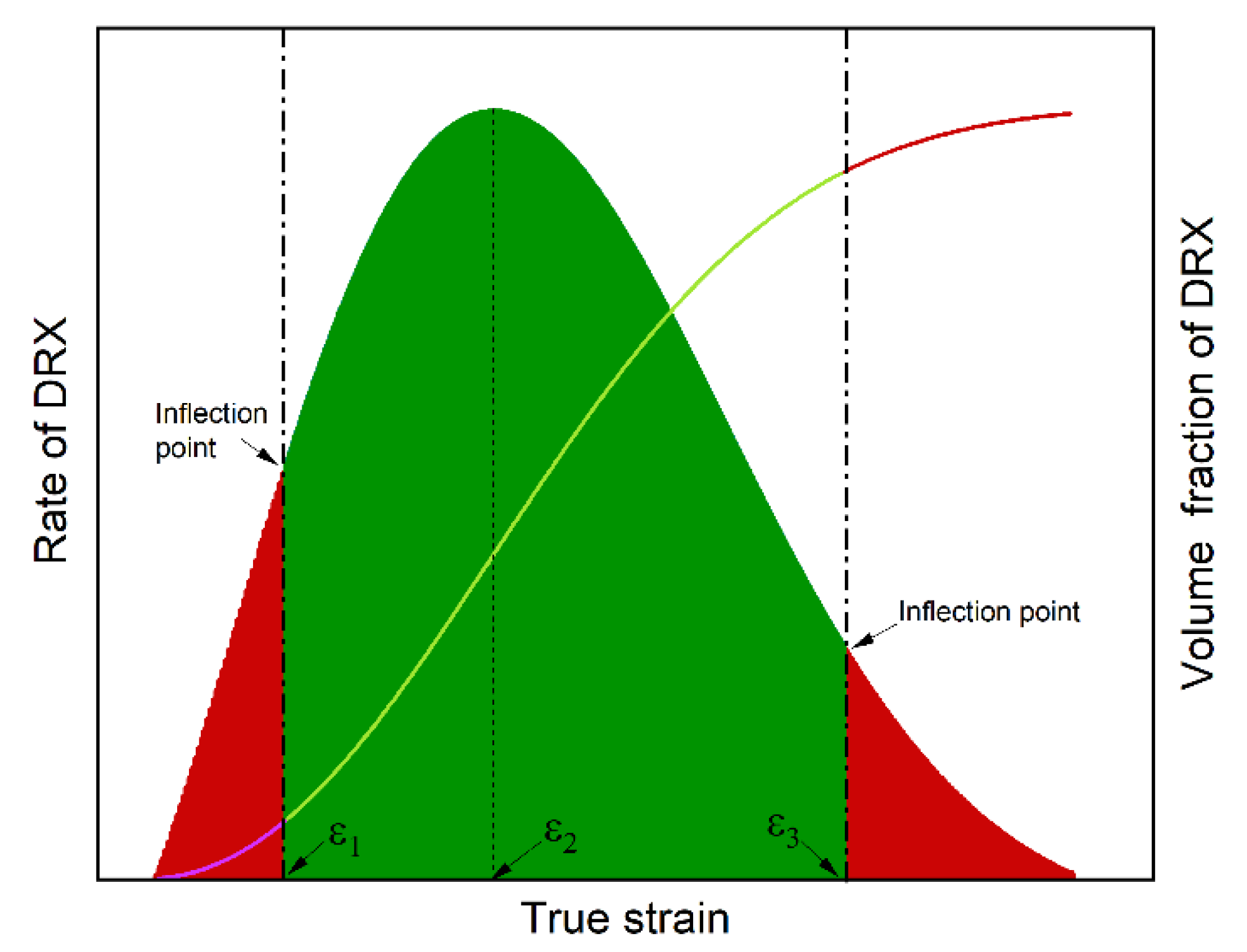
4.2. Determination of Economic Strain (ε₃)

Through Equation (20), the velocity equation of DRX can be expressed by Equation (25) and, furthermore, the quadratic derivative of Equation (25) was constructed and when it is 0:

$$\frac{d{X}_{DRX}}{d\epsilon }=\frac{0.693n}{({\epsilon }_{0.5}-{\epsilon }_c)}(1-X_{DRX}){(\frac{\epsilon -{\epsilon }_c}{{\epsilon }_{0.5}-{\epsilon }_c})}^{n-1}$$

(25)

$$\frac{d^3{X}_{DRX}}{d{\epsilon }^3}=\frac{0.693n}{{({\epsilon }_{0.5}-{\epsilon }_c)}^3}(1-X_{DRX}){(\frac{\epsilon -{\epsilon }_c}{{\epsilon }_{0.5}-{\epsilon }_c})}^{n-3}\left\{\begin{array}{l}{n}^2{\left[0.693{(\frac{\epsilon -{\epsilon }_c}{{\epsilon }_{0.5}-{\epsilon }_c})}^n\right]}^2\\ -3n(n-1)\left[0.693{(\frac{\epsilon -{\epsilon }_c}{{\epsilon }_{0.5}-{\epsilon }_c})}^n\right]\\ -(n-2)(n-1)\end{array}\right\}=0$$

(26)

The solution of Equation (26) is

$$0.693{(\frac{\epsilon -{\epsilon }_c}{{\epsilon }_{0.5}-{\epsilon }_c})}^n=\frac{3n(n-1)\pm n\sqrt{(5n-1)(n-1)}}{2n}$$

(27)

The final strain is expressed as the following equation:

$$\epsilon =\sqrt[n]{\frac{3n(n-1)\pm n\sqrt{(5n-1)(n-1)}}{1.386n}}({\epsilon }_{0.5}-{\epsilon }_c)+{\epsilon }_c$$

(28)

The strain in Equation (28) corresponds to two inflection points of the transform velocity of DRX, the range of which includes the strain corresponding to the maximum velocity of DRX. Thus, there are three key strains, which are rewritten as:

$$\left\{\begin{array}{c}\begin{array}{l}{\epsilon }_1=\sqrt[n]{\frac{3n(n-1)-n\sqrt{(5n-1)(n-1)}}{1.386n}}({\epsilon }_{0.5}-{\epsilon }_c)+{\epsilon }_c\\ \end{array}\\ {\epsilon }_2={\epsilon }_{\begin{array}{l}\max \\ \\ \end{array}}\\ {\epsilon }_3=\sqrt[n]{\frac{3n(n-1)+n\sqrt{(5n-1)(n-1)}}{1.386n}}({\epsilon }_{0.5}-{\epsilon }_c)+{\epsilon }_c\end{array}\right.$$

(29)

The typical transform velocity curve of DRX for X70 pipeline steel is shown in Figure 11, in which it can be divided into three stages based on two inflection points (Equation (29)). In stage I, the DRX process is at the beginning, and the volume fraction and transform velocity of DRX are low, meaning that the developing process of DRX is just beginning. In order for the material to fully undergo DRX behavior, the strain should continue to increase and enter the second stage of recrystallization velocity curve. In stage II, the transition velocity of DRX increases quickly until it reaches the maximum, and then it decreases quickly, which indicates that the maximum transform rate of DRX is located at the second stage. When the strain is around ε_m, the fraction volume of DRX is about 50%, and the mean grain size is rapid and shows uniform refinement. Until the strain increases to ε₃, the volume fraction of DRX is greater than 90%, and the transformation process of DRX is basically completed. When the strain is greater than ε₃, the developing process of DRX has slow velocity, which means that the complete transformation of the remaining approximately 10% of the DRX grains in stage III requires a huge amount of energy and time compared to stage II, resulting in a waste of resources and a decrease in efficiency. In order to obtain optical grain size, enhance production efficiency, and reduce manufacturing cost, ε₃ is the very important economic strain that can guarantee finer and more uniform DRX grains, lower the energy consumption, and provide high production efficiency.

Figure 11. Schematic of velocity curve and volume fraction curve of DRX.

5. Conclusions

In this study, the flow stress–strain curves and DRX kinetic behavior of X70 pipeline steel were investigated using the hot compression tests in a temperature range of 1050~1200 °C and a strain rate range of 0.001~0.1 s⁻¹. The flow stress increases with decreasing temperature and increasing strain rate, and the deformation activation energy is calculated as 358 kJ/mol. Using the relationship between characteristic strain and Z parameter, volume fraction of DRX was established according to the Avrami equation. Furthermore, the flow stress curve predicted by considering the coupling effect of the DRV and DRX processes is in good agreement with experimental results of X70 pipeline steel under different deformation conditions. Finally, through a proposed kinetics model, the most appropriate and economic strain (ε₃) is obtained, which can guarantee fine and uniform equiaxed grain, high production efficiency, and low energy consumption.

References

- Kaikkonen, P.M.; Somani, M.C.; Karjalainen, L.P.; Kömi, J.I. Flow Stress Behaviour and Static Recrystal-lization Characteristics of Hot Deformed Austenite in Microalloyed Medium-Carbon Bainitic Steels. Metals 2021, 11, 138. [Google Scholar] [CrossRef]
- Abarghouee, H.; Arabi, H.; Seyedein, S.; Mirzakhani, B. Modelling of hot flow behavior of API-X70 microalloyed steel by genetic algorithm and comparison with experiments. Int. J. Press. Vessel. Pip. 2020, 189, 104261. [Google Scholar] [CrossRef]
- Devaney, R.J.; Barrett, R.A.; O’Donoghue, P.E.; Leen, S.B. A dislocation mechanics constitutive model for effects of welding-induced microstructural transformation on cyclic plasticity and low-cycle fatigue for X100Q bainitic steel. Int. J. Fatigue 2020, 145, 106097. [Google Scholar] [CrossRef]
- Kumar, A.; Arora, K.S.; Singh, H.; Chhibber, R. Micromechanical modelling of API X80 linepipe steel. Int. J. Press. Vessel. Pip. 2022, 199, 104755. [Google Scholar] [CrossRef]
- Al Shahrani, A.; Yazdipour, N.; Manshadi, A.D.; Gazder, A.; Cayron, C.; Pereloma, E.V. The effect of processing parameters on the dynamic recrystallisation behaviour of API-X70 pipeline steel. Mater. Sci. Eng. A 2013, 570, 70–81. [Google Scholar] [CrossRef]
- Geng, P.; Qin, G.; Zhou, J.; Zou, Z. Hot deformation behavior and constitutive model of GH4169 superalloy for linear friction welding process. J. Manuf. Process. 2018, 32, 469–481. [Google Scholar] [CrossRef]
- Xu, H.; Li, Y.; Li, H.; Wang, J.; Liu, G.; Song, Y. Constitutive Equation and Characterization of the Nickel-Based Alloy 825. Metals 2022, 12, 1496. [Google Scholar] [CrossRef]
- Liu, P.; Zhang, R.; Yuan, Y.; Cui, C.; Zhou, Y.; Sun, X. Hot Deformation Behavior and Workability of a Ni–Co Based Super-alloy. J. Alloys Compd. 2020, 831, 154618. [Google Scholar] [CrossRef]
- Wen, D.; Yue, T.; Xiong, Y.; Wang, K.; Wang, J.; Zheng, Z.; Li, J. High-temperature tensile characteristics and constitutive models of ultrahigh strength steel. Mater. Sci. Eng. A 2020, 803, 140491. [Google Scholar] [CrossRef]
- Ahmadi, H.; Ashtiani, H.R.; Heidari, M. A comparative study of phenomenological, physically-based and artificial neural network models to predict the Hot flow behavior of API 5CT-L80 steel. Mater. Today Commun. 2020, 25, 101528. [Google Scholar] [CrossRef]
- Wu, G.L.; Zhou, C.Y.; Liu, X.B. Dynamic recrystallization behavior and kinetics of high strength steel. J. Cent. South Univ. 2016, 23, 1007−1014. [Google Scholar] [CrossRef]
- Bobbili, R.; Madhu, V. Physically-based constitutive model for flow behavior of a Ti-22Al-25Nb alloy at high strain rates. J. Alloys Compd. 2018, 762, 842–848. [Google Scholar] [CrossRef]
- Han, X.; Yang, J.; Li, J.; Wu, J. Constitutive Modeling on the Ti-6Al-4V Alloy during Air Cooling and Application. Metals 2022, 12, 513. [Google Scholar] [CrossRef]
- Yang, H.; Bu, H.; Li, M.; Lu, X. Prediction of Flow Stress of Annealed 7075 Al Alloy in Hot Deformation Using Strain-Compensated Arrhenius and Neural Network Models. Materials 2021, 14, 5986. [Google Scholar] [CrossRef]
- Zeng, S.; Hu, S.; Peng, B.; Hu, K.; Xiao, M. The constitutive relations and thermal deformation mechanism of nickel aluminum bronze. Mater. Des. 2022, 220, 110853. [Google Scholar] [CrossRef]
- Li, X.-Y.; Zhang, Z.-H.; Cheng, X.-W.; Liu, X.-P.; Zhang, S.-Z.; He, J.-Y.; Wang, Q.; Liu, L.-J. The investigation on Johnson-Cook model and dynamic mechanical behaviors of ultra-high strength steel M54. Mater. Sci. Eng. A 2022, 835, 142693. [Google Scholar] [CrossRef]
- Liu, X.; Ma, H.; Fan, F. Modified Johnson–Cook model of SWRH82B steel under different manufacturing and cold-drawing conditions. J. Constr. Steel Res. 2021, 186, 106894. [Google Scholar] [CrossRef]
- Lin, Y.; Chen, X.-M.; Wen, D.-X.; Chen, M.-S. A physically-based constitutive model for a typical nickel-based superalloy. Comput. Mater. Sci. 2014, 83, 282–289. [Google Scholar] [CrossRef]
- Keller, C.; Hug, E. Kocks-Mecking analysis of the size effects on the mechanical behavior of nickel polycrystals. Int. J. Plast. 2017, 98, 106–122. [Google Scholar] [CrossRef]
- Hariharan, K.; Barlat, F. Modified Kocks-Mecking-Estrin model to account non-linear strain hardening. Metall. Mater. Trans. A 2019, 50, 513–517. [Google Scholar] [CrossRef]
- Avrami, M. Kinetics of phase change. II: Transformation-time relations for random distribution of nuclei. J. Chen. Phys. 1940, 8, 212–224. [Google Scholar] [CrossRef]
- Jonas, J.J.; Quelennec, X.; Jiang, L.; Martin, É. The Avrami kinetics of dynamic recrystallization. Acta Mater. 2009, 57, 2748–2756. [Google Scholar] [CrossRef]
- Hernandez, C.; Medina, S.; Ruiz, J. Modelling austenite flow curves in low alloy and microalloyed steels. Acta Mater. 1996, 44, 155–163. [Google Scholar] [CrossRef]
- Medina, S.F.; Hernandez, C.A. Modelling of austenite in low alloy and microalloyed steels. Acta Mater. 1996, 44, 165–171. [Google Scholar] [CrossRef]
- Yong, M.A.O.; Zhu, D.L.; He, J.J.; Chao, D.E.N.G.; Sun, Y.J.; Xue, G.J.; Yu, H.-F.; Chen, W.A.N.G. Hot deformation behavior and related microstructure evolution in Au− Sn eutectic multilayers. Trans. Nonferrous Met. Soc. China 2021, 31, 1700–1716. [Google Scholar]
- Poliak, E.I.; Jonas, J.J. A one-parameter approach to determining the critical conditions for the initiation of dynamic recrys-tallization. Acta Mater. 1996, 44, 127–136. [Google Scholar] [CrossRef]
- Zener, C.; Hollomon, J.H. Effect of Strain Rate upon Plastic Flow of Steel. J. Appl. Phys. 1944, 15, 22–32. [Google Scholar] [CrossRef]
- Laasraoui, A.; Jonas, J.J. Prediction of steel flow stresses at high temperatures and strain rates. Met. Mater. Trans. A 1991, 22, 1545–1558. [Google Scholar] [CrossRef]
- Wang, L.; Liu, F.; Zuo, Q.; Chen, C.F. Prediction of flow stress for N08028 alloy under hot working conditions. Mater. Design 2013, 47, 737–745. [Google Scholar] [CrossRef]
- Wang, L.; Liu, F.; Zuo, Q.; Chen, C.F. Modeling Dynamic Recrystallization Behavior in a Novel HIPed P/M Superalloy during High-Temperature Deformation. Materials 2022, 15, 4030. [Google Scholar] [CrossRef]
Publisher’s Note: MDPI stays neutral with regard to jurisdictional claims in published maps and institutional affiliations. |
© 2022 by the authors. Licensee MDPI, Basel, Switzerland. This article is an open access article distributed under the terms and conditions of the Creative Commons Attribution (CC BY) license (https://creativecommons.org/licenses/by/4.0/).