1. Introduction
The global population growth rate was estimated to be about 1.096% in 2012 [
1]. This rapid development of the human population, increased number of buildings and technological advancement in energy-intensive applications are causing fast electric energy consumption growth [
2]. The traditional fossil fuel-based energy generation increases the emissions of greenhouse gases, and as a result, green energy generation technologies are adapted. Similarly, many incentives are being implemented to help the development of clean energy [
3].
Renewable energy generation output is hard to control due to its intrinsic intermittency and uncontrollable primary energy source (wind, sun, tides) [
4]. As a result, wind, solar or other renewable energy generation requires a large amount of backup power to compensate variability [
5]. The traditional fossil fuel-based spinning reserve would contradict the aim to lower carbon emissions, so other solutions are needed.
There are two primary ways to avoid, if not minimise, the renewable energy balancing issue. For example, large-scale energy storage facilities could help to shift energy in time, but this requires a large amount of investment and usually high maintenance and running costs [
5,
6,
7]. Secondly, interconnectivity could lower the total generated power variability. The larger the system, the lower the statistical variation and volatility of the total generation and consumption of electricity [
8], as long as there is no significant correlation between intermittent energy outputs [
9]. In general, interconnected geographically-distant generating units have lower correlation, thus total power variability is reduced.
There are also other techniques to strengthen system backup; however, the forecasting analyses represented in this paper are aimed to serve the required information for future development of demand-side management (DSM). This paradigm potentially aims to solve the energy balancing problem from the consumer side instead of actively controlling the generation and transmission [
10]. It has the potential to increase system efficiency and power quality, while reducing system vulnerability and, hence, helping to conserve energy [
8].
Demand-side management is a concept related to the control of residential and industrial appliances to maximise the use of energy. The DSM term was publicly introduced in the early 1980s [
11], though a lack of IT and communication infrastructure limited its full potential until the early 21st century. It involves peak shaving, valley filling, load shifting and other load profile transforming techniques [
12,
13]. End users could participate in DSM through price-based DSM programs (lower tariffs), direct control-based programs (various incentives or benefits to the user in return) or partial direct control (the user would release control during certain non-predefined times). End users tolerate different discomfort levels, thus individual agreements are needed between the system operator and the consumer.
Residential appliances could be classified as shiftable and non-shiftable loads. For example, lighting is a non-shiftable category, because it would greatly degrade comfort if not used when needed by the user. On the other hand, users are not very sensitive to small changes, such as the temperature setpoint of a hot water heater. Hot water heaters are commonly-used devices in most houses, where water has a large specific heat capacity enabling control relatively easily. Previous research suggests that domestic hot water (DHW) accounts from 7.5% to 40% [
14,
15] of total domestic energy usage. These properties make hot water heaters a perfect candidate appliance to participate in DSM and system balancing [
16,
17,
18], hence, the need to focus on hot water demand forecasting.
Currently most hot water tanks are controlled in a very archaic way: Water is maintained at a constant temperature setpoint. It is obvious that there are patterns of hot water usage profiles, and water should not be kept at its highest temperature at all times. The authors of this paper propose that it is possible to forecast individual dwelling hot water consumption profiles and, hence, to potentially participate in DSM. By knowing when hot water is needed, it is then possible to lower the setpoint temperature at certain times [
19]. This would enable the water heater appliance to participate in a DSM program. For example, there would be a range of temperatures in which water could be varied, thus changing each individual’s electricity consumption profile to reach the system balance [
20]. If the range of comfortable temperatures is wide, the appliance has more flexibility in responding to DSM. Therefore, there is a key need for accurate individual hot water consumption forecasts, which is researched in this study.
The section above indicates the need for DHW forecasts and the potential of DHW being used in DSM applications. The remainder of the paper is focused on analysing and predicting time series data. The work is organized as follows. In
Section 2, previous studies are reviewed and the need for individual DHW consumption forecasts is indicated.
Section 3 describes data preparation, model selection and performance evaluation. In
Section 4, the data are analysed, including tests for time series stationarity and seasonality.
Section 5 shows the results of model performances, and
Section 6 overviews the findings. The work is concluded in
Section 7.
2. Previous Studies
This section reviews the previous research related to hot water consumption forecasts. The first part includes studies focused on forecasting electricity demand caused by DHW, whereas the second part reviews research related to forecasting thermal demand and demand response (DR).
Sandels
et al. [
21] presented a simulation model for DHW that forecasts load profile. The DHW module is based on non-homogeneous Markov chains, where occupants change states within certain probabilities overtime. Those states correspond to certain activities at home that require a specific amount of energy. Only two activities, taking showers or baths, were taken into account, although there are other ways that hot water consumption could occur, for example hand washing or manual dish washing. Heat loss from the hot water tank was also taken into account.
Some other researchers [
2] demonstrated electrical energy forecasting using artificial intelligence (AI). Support vector machine (SVM) and artificial neural network (ANN) methods were considered, including hybrids of both. Furthermore, some others used SVM and ANN to forecast 24-h electricity loads for individual houses [
20]. Javed
et al. also used ANN to predict the load and compared model performances with the results of traditional model, such as generalized autoregressive conditional heteroskedasticity (GARCH) model, exponential smoothing (ETS) and multiple linear regression [
8]. They stressed the importance of individual forecasts with no data aggregation between houses. The use of ANN was also demonstrated by Bartecsko-Hibbert
et al. to predict the temperature characteristics of DHW [
14].
Simple forecasting techniques are required in order to compare the relative performances of a more sophisticated model and to serve as a benchmark. For example, De Felice and Yao demonstrated short-term load forecasting and chose naive seasonal model as a benchmark [
22]. Although the paper presented a forecasting technique for the total load demand profile using hot water consumption only as external inputs, it demonstrated that ANN and seasonal autoregressive integrated moving average (ARIMA) models could be used to deliver short-term energy forecasting.
Negnevitsky and Wong developed an evaluation tool for a DSM hot water system in [
14]. It is capable of simulating the energy peak-shaving technique using unique multi-layer thermally-stratified hot water cylinders. Monte Carlo simulations were used to generate hot water load profiles for the residential users.
The use of DHW control for DSM and peak shaving is also demonstrated in [
23]. Hashem Nehrir
et al. demonstrated how aggregate electric water heater loads could be controlled to lower the maximum power demand for certain time periods using voltage control. Researchers emphasised the use of aggregated data, focused on control during critical hours, and demonstrated how residential hot water demand management can enhance the power quality and reliability of the overall system.
Popescu and Serban in [
24] presented domestic hot water consumption forecasting using time series models. The authors were using real world data collected from a block of flats with 60 apartments. It demonstrated that the Box-Jenkins model is capable of forecasting aggregated total thermal power demand for different days of the week.
Bakker
et al. in [
25] showed that domestic heat demand prediction is crucial for the adoption of micro combined heat and power (micro-CHP) appliance clusters. They used ANN with the input of the previous day and previous week heat demand profile, as well as weather information to predict 24-h ahead.
The authors in [
26] show a very recent work based on forecasting volumetric hot water needs at an individual house level. The paper considers eight residences, 30-min resolution and a 12-week model training period. The proposed autoregressive moving average (ARMA) model is compared to the (a) benchmark mean model and (b) moving average on the same day of the week during the last two months [
27]. It is concluded that the ARMA model gives higher precision and better recovery from large variations (holidays). The authors also stress the need for residential DHW consumption forecasts to enable precise demand response.
Neves and Silva in [
28] studied the optimal electricity dispatch in a grid consisting of hybrid diesel, renewable generation and the demand response technique for distributed thermal storage. The authors have tested different demand response strategies based on heuristics, linear programming and genetic algorithms. The DHW storage tank model is presented using the energy balancing technique. This leads to the model being lossless and fully mixed.
There is an extensive amount of previous research done on forecasting thermal energy needs as summarised in this section. Most of it investigates consolidated data of a group of consumers. Such data aggregation improves the forecasting performance, but has a disadvantage of concealing the users’ individuality. This paper investigates individual hot water consumption profile forecasts, which discloses the diversity of hot water usage at a given time between different consumption locations, which might potentially be beneficial for DSM. The demonstrated methods (such as exponential smoothing, seasonal autoregressive moving average and seasonal decomposition) incorporate confidence levels, which might be used to avoid compromising user’s comfort. Another advantage of the forecasting methods used in this paper is the low computational power requirements. Predictions should be computed locally at smart devices, so the requirements for processing capabilities are strict. Advanced forecasting methods, such as ANN, are generally relatively less robust and computationally more expensive, compared to traditional exponential smoothing, ARIMA or seasonal decomposition [
29].
3. Methodology
This section will describe the general methodology and techniques used in the data preparation, the model design, the evaluation and the comparison of forecast models.
3.1. Preparation of the Data
The data were collected by the Energy Monitoring Companyin conjunction with and on behalf of the Energy Saving Trust with funding of the Sustainable Energy Policy Division of the Department of Environment, Food and Rural Affairs (Defra), UK [
30]. The initial dataset contained hot water consumption measurements from about 120 residential houses. The records included temperature information from various locations, where hot water was supplied. Total volumetric consumption was also measured. The data were collected during the years 2006 and 2007.
By visual inspection, some of the datasets were discarded due to erroneous measurements. As a result, there were 95 datasets left. Outliers, as well as any other inconsistencies in the measurements, supposedly from “stuck” sensors, were also discarded.
The sampling rate of initial data was not constant. Measurements were recorded every 10 min, but when a run-off was detected, the sampling rate increased to 5 s. Before any analysis started, the data were resampled at hourly intervals, by aggregating the volumetric consumption of every hour.
The preparation of the data resulted in obtaining 95 month-long, 1-hour resolution time series of a volumetric hot water consumption at different households. In addition, the aggregate dataset was also generated for comparison reasons, containing the average hot water consumption from 95 dwellings. The separate consumption profiles were normalised using the standard deviation before taking the arithmetic mean.
3.2. Forecasting Models
It is a general practice to compare model performance with standard simple benchmark models [
22]. The authors have chosen mean, simple and seasonal naive benchmark models to be compared to the models developed in this paper. The mean forecasting model computes the values of the horizon by taking the arithmetic average of past values. The simple naive model basically assumes that every future forecast is equal to the most recent value observed. These two models have been chosen as a baseline for forecasting. Since the data are exclusively periodic due to the fact that people tend to have habits, there should be seasonality in the benchmark model. For this reason, the authors have decided to use the seasonal naive model, which computes forecasts by observing the value at the same time in the previous season [
31]. In this paper, there are two seasonal periods considered: a day-long period and a week-long period.
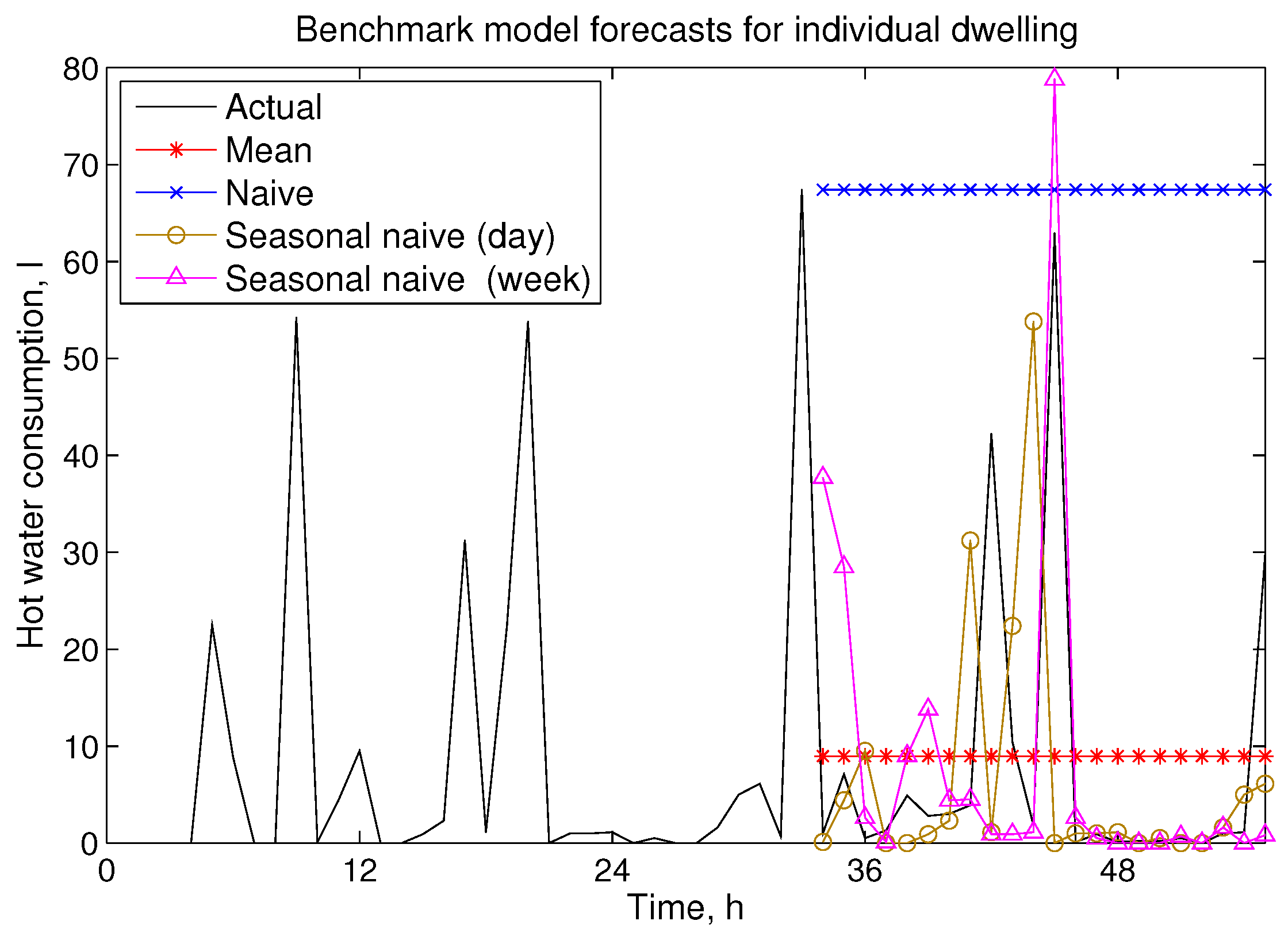
Figure 1 illustrates the performance of benchmark models for single house hot water consumption. It can be seen that both the mean and naive models do not perform well for 24 h ahead forecasting. A better performance is observed from seasonal naive models, and this suggests that seasonality plays a key role.
Figure 1.
Exemplar benchmark model forecasts for an individual dwelling.
Figure 1.
Exemplar benchmark model forecasts for an individual dwelling.
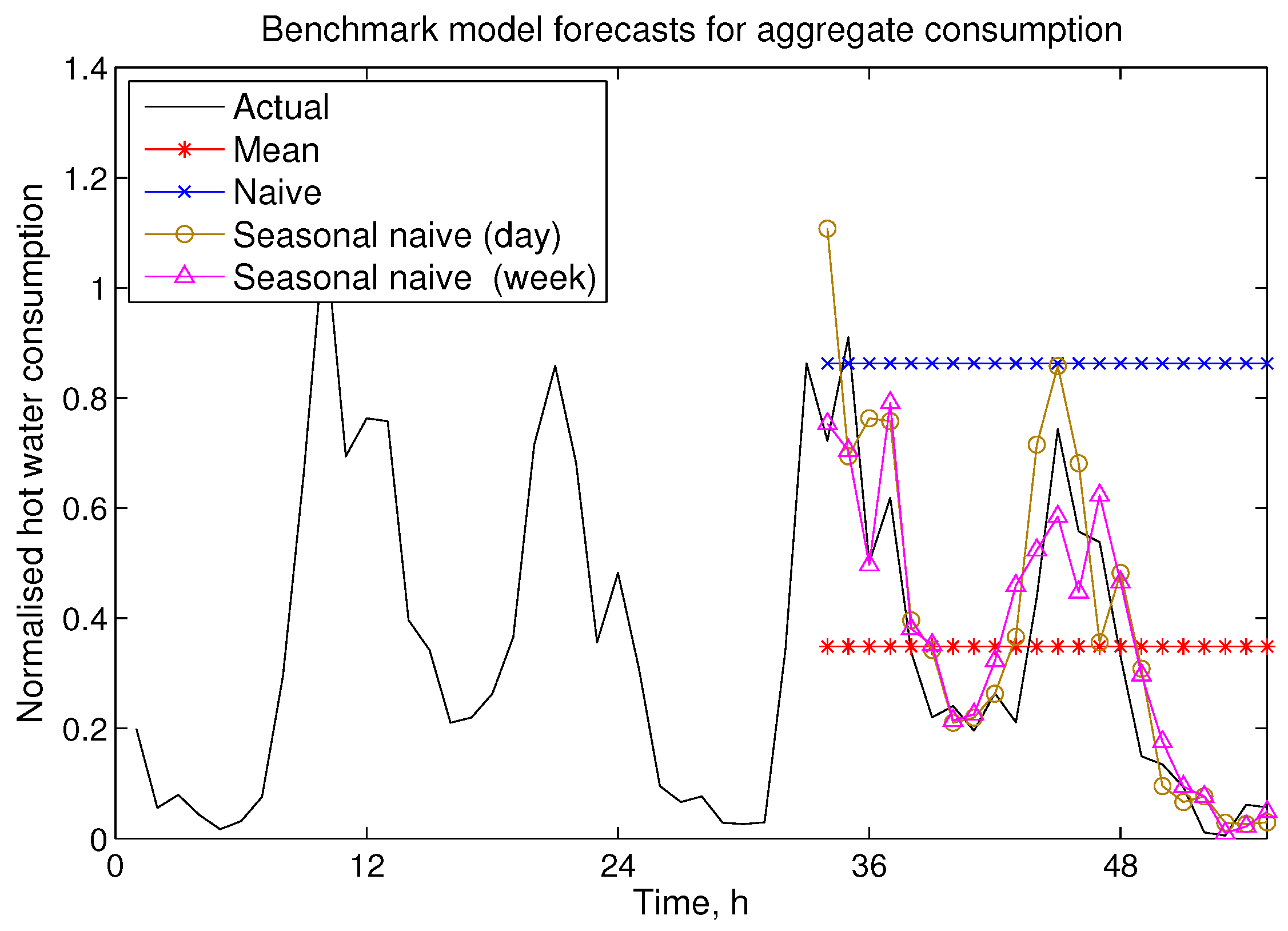
Figure 2 shows an example forecast for total hot water consumption. Since this time series involves information from many consumers, the aggregate profile is more stable and repetitive compared to profiles from individual dwellings, thus seasonal naive models perform reasonably well. In this paper, all other models will be compared to the seasonal naive (daily) model. Both individual and aggregate data were fitted to a number of models: exponential smoothing (ETS), seasonal autoregressive integrated moving average (ARIMA), seasonal decomposition of time series by Loess model (STL) and a combination of them.
Figure 2.
Exemplar benchmark model forecasts for aggregate hot water consumption.
Figure 2.
Exemplar benchmark model forecasts for aggregate hot water consumption.
The exponential smoothing state space models are fitted using the R software environment. It offers an automated model selection and fitting tool. The notation in this paper follows the ETS() function from R. The three parameters are the error, trend and seasonal components and can be additive (A), multiplicative (M) or none (N). The best performing model parameters are chosen using the information criterion. The combinations of these correspond to different models, but this is out of the scope of this paper [
31,
32]. The results showed that for individual forecasts, the best performing model was ETS(A,N,A) for every dwelling. For the aggregate consumption case, the best results were shown by the ETS(M,N,M) model.
The seasonal autoregressive integrated moving average is a well-established modelling technique, better known as the Box-Jenkins methodology. A series of models were fitted using the ARIMA() function in R software [
32]. It chooses the parameters for the best fitting model according to either the Akaike information criterion (AIC), the corrected Akaike information criterion (AICc) or the Bayesian information criterion (BIC). These parameters are:
p, the number of autoregressive terms;
d, the number of non-seasonal differences needed for stationarity;
q, the number of lagged forecast errors in the prediction equation;
P, the seasonal autoregressive terms;
D, the number of seasonal differences;
Q, the number of seasonal lagged forecast errors in the prediction equation.
Model orders were not fixed; thus, different dwellings were assigned to the best performing ARIMA models. The model order distribution is then calculated and compared to the parameters of the aggregate time series model.
The seasonal decomposition of time series split the time series into seasonal, trend and irregular parts by Loess. At first, the seasonality is removed using Loess by smoothing the seasonal sub-series. The remainder is then smoothened to find the trend. A combination of STL and ETS or ARIMA was also used. The time series were first decomposed, then the forecasting model was fitted to the seasonally adjusted data, and finally, the datasets were re-seasonalised.
The main factors affecting the accuracy of the forecast are the data aggregation level, the forecasting horizon and the time series sparsity. In this paper, both individual and aggregate demand profiles are forecasted using 10 different models. It should be noted that single house hourly water usage time series are very sparse. The aggregate data, on the other hand, contain far less zeros. It is expected to get much better forecasts for average consumption profiles compared to individual houses. The forecasting horizon is up to 24 h for all data series.
3.3. Performance Evaluation
There are many possible ways to measure how well the forecasting models perform. The most general practice is to compare mean absolute error (MAE) or root mean square error (RMSE), which are scale-dependent measures. Since different dwellings accommodate a different number of people and their water usage habits vary, absolute measures need to be either normalised or, alternatively, relative measures need to be taken. To normalise MAE and RMSE, a standard deviation (SD) of measurements was used. As a result, normalised MAE and normalised RMSE could be calculated as follows:
where
is the forecast error and
is the target value. Functions
and
are the arithmetic average and the standard deviation, respectively.
Mean absolute percentage error (MAPE) could be another possible choice for performance evaluation; however, hot water consumption time series are very sparse, and errors are compared to zero values, making the calculations unstable. This makes MAPE unsuitable in this application. The method proposed by Hyndman and Koehler in [
31] suggests comparing the errors given by the forecasting models to the errors from seasonal naive benchmark models to overcome this issue. The scaled errors would then be defined as:
where
is the scaled error,
is the forecast error,
T is the time series length,
s is the season parameter and
y is the set of target values. The seasonal parameter is equal to 24 h in this comparison. The mean absolute scaled error (MASE) is defined by Equation (
4):
In addition, the authors of this paper have measured the regression value R as another way of assessing the model’s performance. It is the regression value of the one-step-ahead forecast versus the target value. All other performance measures were also calculated using one-step-ahead forecasts from test datasets.
5. Results
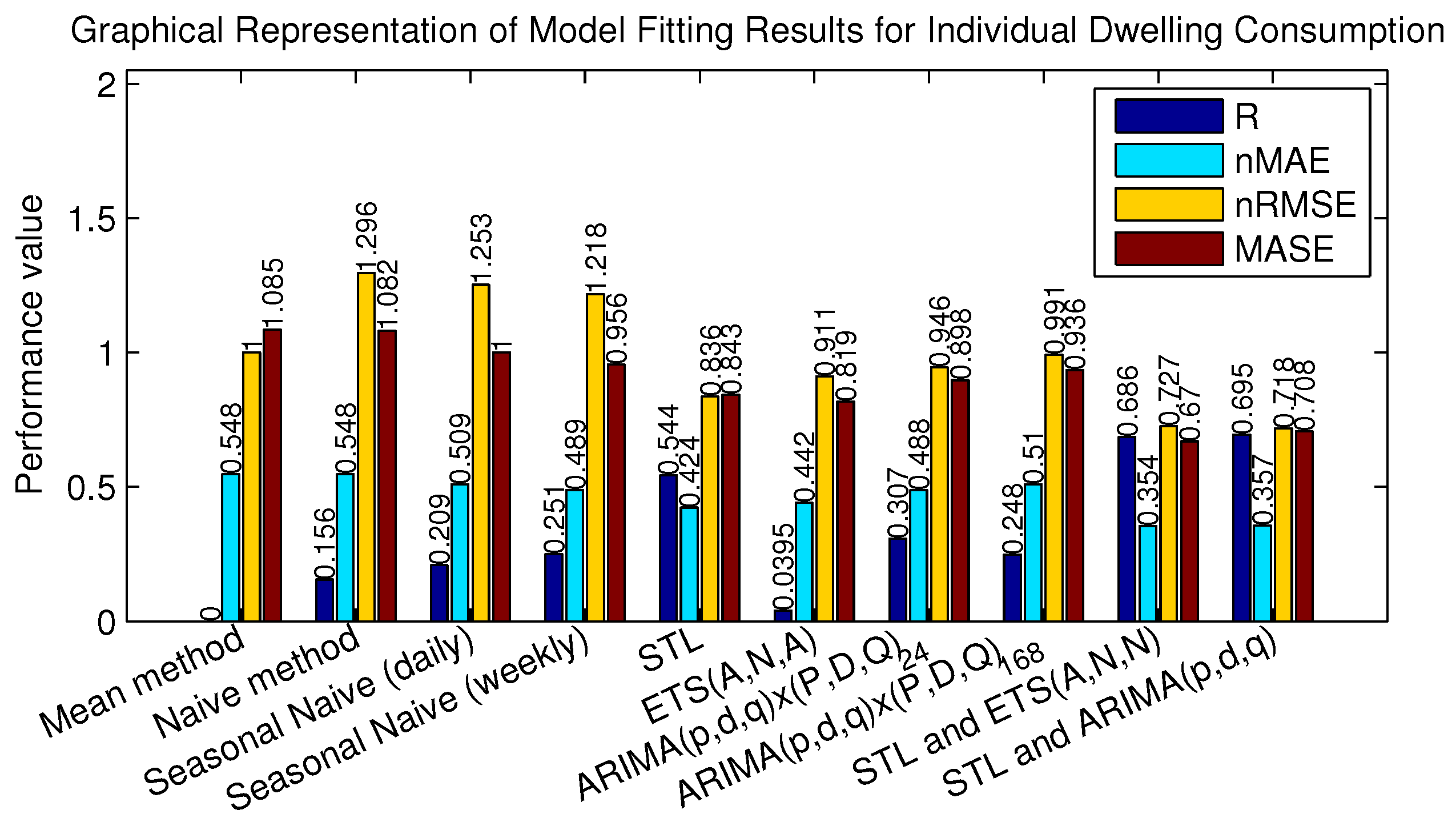
The forecasting results of hot water usage in individual dwellings are positive and promising. Every forecasting method outperformed the chosen benchmark models.
Table 2 and
Figure 7 summarise how well the models performed by showing the average performance measures from the best fitting model for every dwelling. For a particular dwelling, the best-performing models were chosen by adjusting the parameters, for example
p,
d and
q values in the ARIMA model were chosen using the Akaike or the Bayesian information criterion [
32]. A standard deviation is also presented showing how much performance measures differ between houses. It can be seen that seasonal decomposition in conjunction with exponential smoothing (STL and ETS(A,N,N)) and ARIMA (STL and ARIMA(
p,
d,
q)) perform the best. On average, they perform more than 30% better than the seasonal naive benchmark model.
Table 2.
Model fitting results for individual dwelling consumption. MASE, mean absolute scaled error; STL, seasonal decomposition of time series by Loess; ETS, exponential smoothing.
Table 2.
Model fitting results for individual dwelling consumption. MASE, mean absolute scaled error; STL, seasonal decomposition of time series by Loess; ETS, exponential smoothing.
| Method | Performance Measures |
|---|
| R (SD) | nMAE (SD) | nRMSE (SD) | MASE (SD) |
|---|
| Mean method | 0.000 (0.000) | 0.548 (0.097) | 1.000 (0.000) | 1.085 (0.145) |
| Naive method | 0.156 (0.084) | 0.548 (0.109) | 1.296 (0.067) | 1.082 (0.142) |
| Seasonal naive (daily) | 0.209 (0.117) | 0.509 (0.095) | 1.253 (0.098) | 1.000 (0.000) |
| Seasonal naive (weekly) | 0.251 (0.126) | 0.489 (0.106) | 1.218 (0.109) | 0.956 (0.073) |
| STL | 0.544 (0.072) | 0.424 (0.056) | 0.836 (0.053) | 0.843 (0.061) |
| ETS(A,N,A) | 0.395 (0.112) | 0.442 (0.070) | 0.911 (0.055) | 0.819 (0.096) |
| ARIMA(p,d,q)×(P,D,Q) | 0.307 (0.112) | 0.488 (0.081) | 0.946 (0.039) | 0.898 (0.067) |
| ARIMA(p,d,q)×(P,D,Q) | 0.248 (0.113) | 0.510 (0.092) | 0.991 (0.092) | 0.936 (0.065) |
| STL and ETS(A,N,N) | 0.686 (0.056) | 0.354 (0.052) | 0.727 (0.057) | 0.670 (0.041) |
| STL and ARIMA(p,d,q) | 0.695 (0.054) | 0.357 (0.053) | 0.718 (0.056) | 0.708 (0.045) |
Figure 7.
Graphical representation of
Table 2.
Figure 7.
Graphical representation of
Table 2.
Table 3 shows the parameter distributions of the best fitting seasonal and non-seasonal ARIMA models. The first order parameter is the most common. Model selection resulted in about 60% of the time series requiring first order differentiating in order to be stationary. This complies with the stationarity test results that were previously conducted. On the other hand, seasonal differencing is not required according to stationarity tests and model fitting results (none of the best fitting models required seasonal differencing).
Table 3.
Seasonal ARIMA model orders.
Table 3.
Seasonal ARIMA model orders.
| Method | Parameters (Orders) |
|---|
| p | d | q | P | D | Q |
|---|
| ARIMA(p, d, q)×(P, D, Q) | 0%–22%
1%–40%
2%–30%
3%–7%
4%–1% | 0%–40%
1%–60% | 0%–15%
1%–36%
2%–32%
3%–10%
4%–7% | 0%–31%
1%–41%
2%–28% | 0%–100% | 0%–21%
1%–21%
2%–58% |
| ARIMA(p, d, q)×(P, D, Q) | 0%–29%
1%–34%
2%–28%
3%–7%
4%–2% | 0%–40%
1%–60% | 0%–29%
1%–37%
2%–24%
3%–9%
4%–1% | 0%–51%
1%–39%
2%–10% | 0%–100% | 0%–49%
1%–51% |
| STL and ARIMA(p,d,q) | 0%–8%
1%–36%
2%–30%
3%–14%
4%–12% | 0%–37%
1%–63% | 0%–10%
1%–25%
2%–33%
3%–20%
4%–12% | N/A | N/A | N/A |
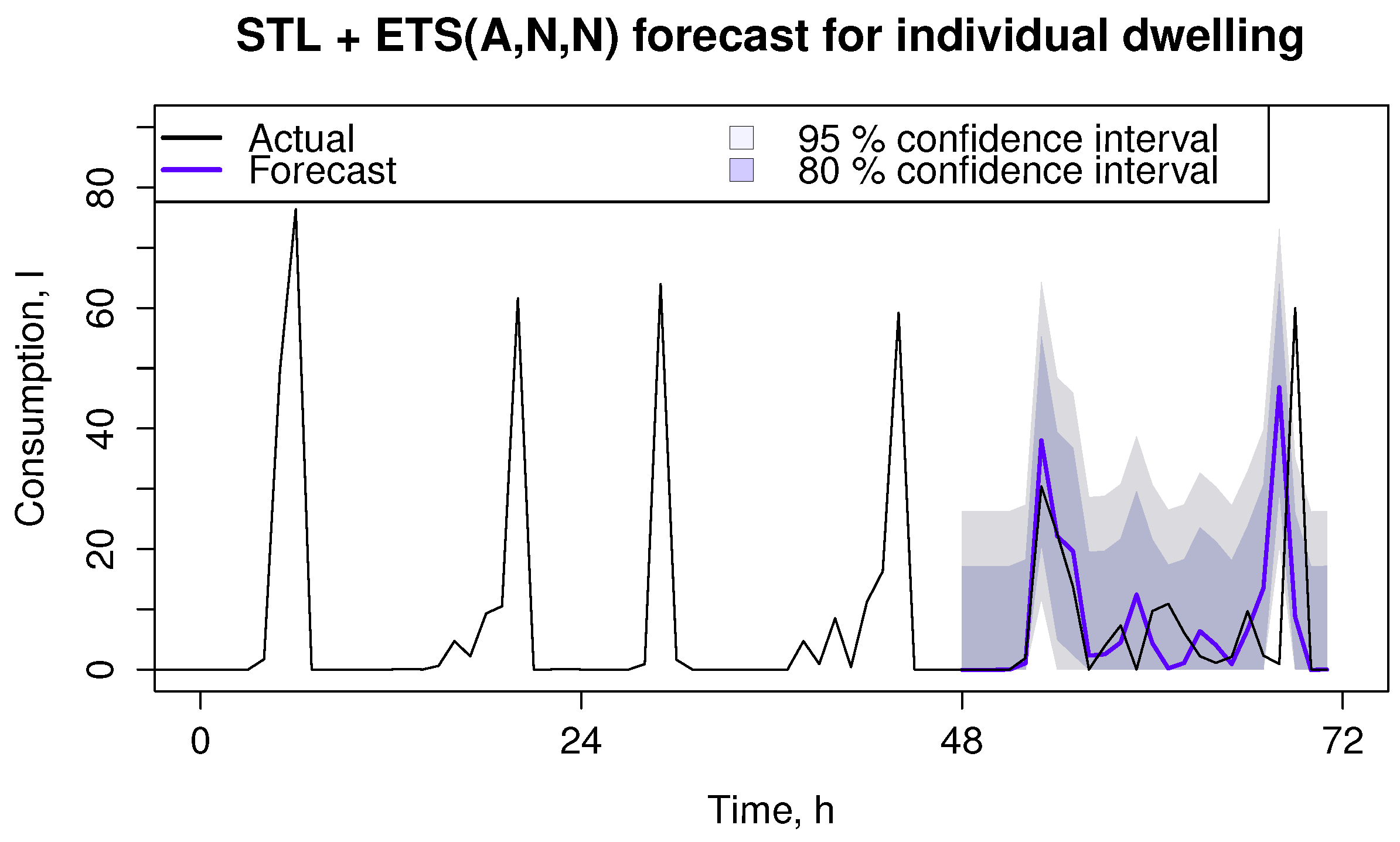
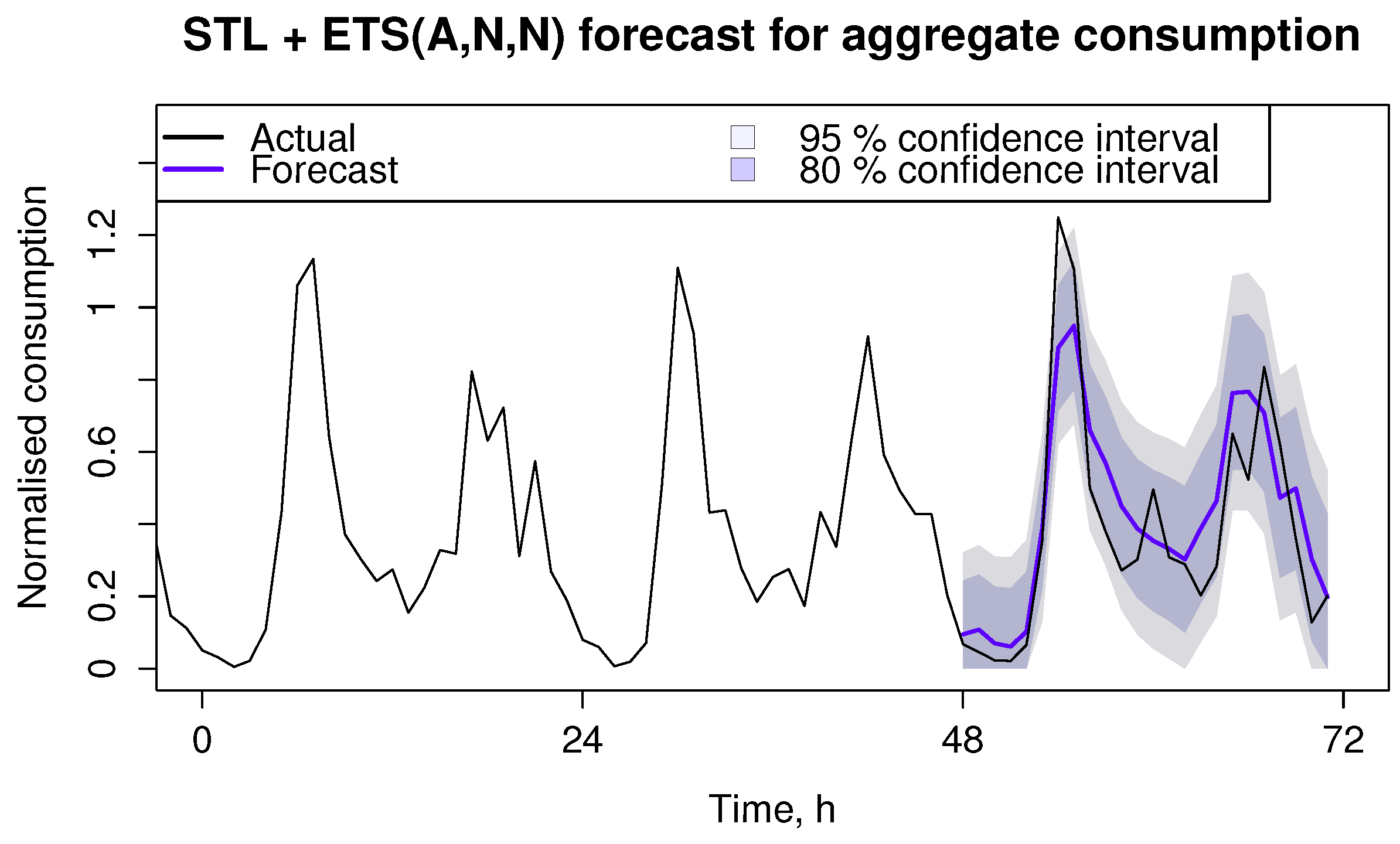
Two exemplar forecasting cases have been plotted.
Figure 8 and
Figure 9 demonstrate 24 h ahead forecast together with 80% and 95% confidence intervals.
Figure 8.
Best performing method for non-aggregate time series.
Figure 8.
Best performing method for non-aggregate time series.
Figure 9.
Best performing method for aggregate time series.
Figure 9.
Best performing method for aggregate time series.
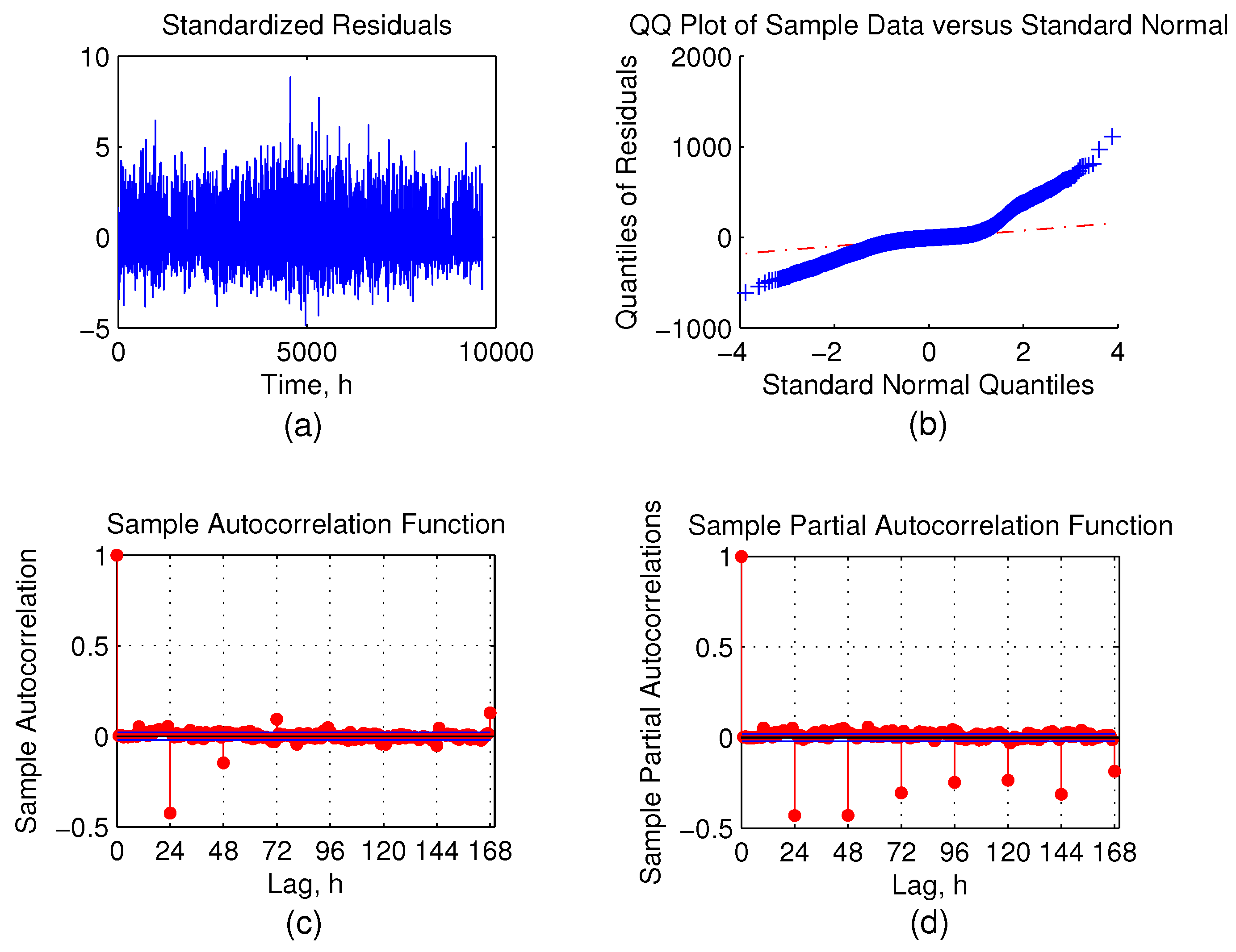
Residual analysis plots for exemplar cases can be found in
Figure 10 and
Figure 11. They depict the distribution of errors using the Q-Q plot by plotting the distribution of residual errors
versus the normal distribution. The bottom part of the figure shows the residual error ACF and PACF plots.
Figure 10.
Residual analysis for the single dwelling consumption forecast. (a) Standardised residuals; (b) Q-Q plot of residuals; (c) ACF of residuals; (d) PACF of residuals.
Figure 10.
Residual analysis for the single dwelling consumption forecast. (a) Standardised residuals; (b) Q-Q plot of residuals; (c) ACF of residuals; (d) PACF of residuals.
Figure 11.
Residual analysis for mean consumption forecast. (a) Standardised residuals; (b) Q-Q plot of residuals; (c) ACF of residuals; (d) PACF of residuals.
Figure 11.
Residual analysis for mean consumption forecast. (a) Standardised residuals; (b) Q-Q plot of residuals; (c) ACF of residuals; (d) PACF of residuals.
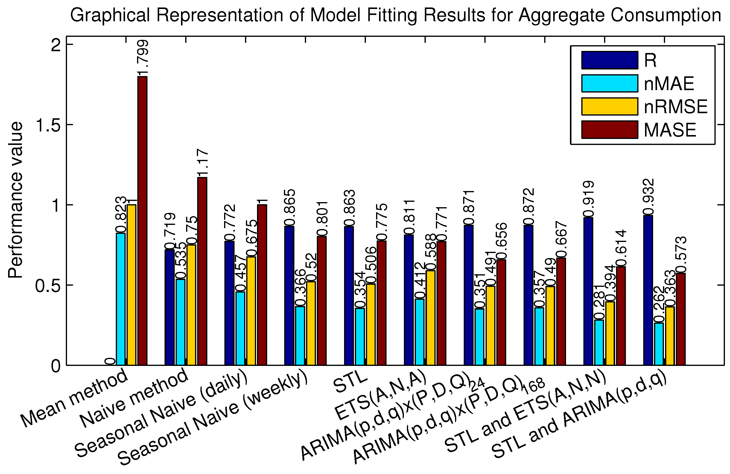
Finally,
Table 4 and
Figure 12 show the performance results for aggregate consumption forecasts. Both individual and aggregate consumption forecasts were computed using similar models so that the result could be compared asily.
Table 4.
Model fitting results for aggregate consumption.
Table 4.
Model fitting results for aggregate consumption.
| Method | Performance Measures |
|---|
| R | nMAE | nRMSE | MASE |
|---|
| Mean method | 0.000 | 0.823 | 1.000 | 1.799 |
| Naive method | 0.719 | 0.535 | 0.750 | 1.170 |
| Seasonal naive (daily) | 0.772 | 0.457 | 0.675 | 1.000 |
| Seasonal naive (weekly) | 0.865 | 0.366 | 0.520 | 0.801 |
| STL | 0.863 | 0.354 | 0.506 | 0.775 |
| ETS(M,N,M) | 0.811 | 0.412 | 0.588 | 0.771 |
| ARIMA(1,1,1) × (1,0,2) | 0.871 | 0.351 | 0.491 | 0.656 |
| ARIMA(1,1,2) × (1,0,0) | 0.872 | 0.357 | 0.490 | 0.667 |
| STL and ETS(A,N,N) | 0.919 | 0.281 | 0.394 | 0.614 |
| STL and ARIMA(3,1,1) | 0.932 | 0.262 | 0.363 | 0.573 |
Figure 12.
Graphical representation of
Table 4.
Figure 12.
Graphical representation of
Table 4.
6. Discussion
By comparing
Table 2 and
Table 4, it can be seen that the aggregate consumption profile is more predictable than individual consumption profiles. The best MASE for aggregate data is 0.573 compared to the MASE of 0.670 for separate house forecast. Normalised RMSE is about two times less for mean consumption data, where approximately 30% improvement is seen on the R value and normalised MAE. As mentioned in
Section 3.3, the scale of consumption profiles differs between dwellings due to different numbers of occupants and water usage habits, so it is best to measure performance by looking at relative figures. Nevertheless, mean absolute errors were calculated for all individual forecasting performances and are in a range of 4.4 to 6.9 L/h. The best performing model (STL and ETS(A,N,N)) corresponds to an error of 4.4 L/h.
Consumption peaks in individual dwellings are very high and narrow (on some occasions, consumption changes from zero to 100 L and back to zero in three consecutive hours), meaning the consumption is very concentrated in time. When the repetitive water usage is in between two consecutive hours, it is very hard to predict at which hour the peak will appear. Due to this extreme behaviour and sparse time series, forecasting becomes very time sensitive, i.e., if the forecast is off by one single time step, the performance measures drop dramatically, and the confidence intervals increase.
This problem worsens for higher resolution forecasts. The authors found that a resolution of one hour gives the best trade-off between forecast accuracy and the need to have sub-hour information. Various DR programs are designed to respond for up to sub-minute power fluctuations. It must be noted that although this paper describes hourly hot water consumption forecasts, the potential demand response program might be of a higher resolution, which is mainly limited by the communication channel parameters. The hot water consumption forecasts could potentially be used for deciding whether a particular water heater is capable of responding to a particular period of time.
The confidence intervals show the probability of the forecast to be accurate, i.e., wider intervals mean less confident forecasts. It can be seen that individual dwelling consumption forecasts produce wider confidence intervals than aggregate consumption forecasts, meaning it is harder to confidently predict individual hot water usage as opposed to total collaborative usage. The ability to predict DHW usage at the individual house level is the key to successful DSM program implementation. Although the confidence intervals suggest that there could always be a fair amount of water usage, the model accurately predicts the time of high demand periods. On the other hand, the forecast for mean consumption is more accurate compared to individual consumption, and the confidence intervals are narrower, due to consumer diversity.
The Q-Q plot demonstrates that the residual errors follow a normal distribution quite well, which means that residuals are mostly white noise and the model incorporates enough information to predict ahead. There is a fair amount of error autocorrelation at multiples of 24-h lags in
Figure 10, bottom. This could be explained by closely examining error time plots and is related to time series being sparse. There is a clear pattern of a high and a low probability for errors. During the night, the consumption reduces to the minimum, and the resulting errors are also small. The opposite happens during the peak consumption. This behaviour makes the error autocorrelation inevitable at multiples of 24.
7. Conclusions
In conclusion, the increased global energy consumption and the expansion of intermittent renewable generation require new electricity balancing tools. The DSM technologies have huge potential to use distributed water heaters as energy shifting devices for solving this energy balancing problem.
The main goal of this paper was to research the possibility of forecasting hot water volumetric consumption at an individual dwelling level. DSM programs that incorporate forecasts tailored to individual houses can respond to energy surplus or shortage more reliably and, hence, perform better.
This paper also analysed hot water consumption profiles for 95 individual dwellings and aggregate information. Strong daily and weekly usage patterns were detected; hence, seasonal forecasting models were used. The forecasting techniques were applied to acquire 24 h ahead forecasts using estimated exponential smoothing, ARIMA and seasonal decomposition models. The results show that chosen prediction methods could be potentially used for DSM applications to control hot water consumption possibly without compromising user’s comfort. The best performing models were discovered to be “STL and ETS(A,N,N)” and “STL and ARIMA(p,d,q)”.
Future work might include taking into account time of the year (yearly seasonality), total number of occupants, as well as the number of children, weather information and information from the user (set of holiday dates). Furthermore, as future work, these forecasts could be tested in the context of DSM and DR.


