Maximum Energy Output of a DFIG Wind Turbine Using an Improved MPPT-Curve Method

Abstract

A new method is proposed for obtaining the maximum power output of a doubly-fed induction generator (DFIG) wind turbine to control the rotor- and grid-side converters. The efficiency of maximum power point tracking that is obtained by the proposed method is theoretically guaranteed under assumptions that represent physical conditions. Several control parameters may be adjusted to ensure the quality of control performance. In particular, a DFIG state-space model and a control technique based on the Lyapunov function are adopted to derive the control method. The effectiveness of the proposed method is verified via numerical simulations of a 1.5-MW DFIG wind turbine using MATLAB/Simulink. The simulation results show that when the proposed method is used, the wind turbine is capable of properly tracking the optimal operation point; furthermore, the generator’s available energy output is higher when the proposed method is used than it is when the conventional method is used instead.

1. Introduction

Generally, generator wind turbines are divided into two groups: fixed-speed wind turbines (FSWT) and variable-speed wind turbines (VSWT). For FSWTs, a squirrel-cage induction generator (SCIG) [1] is often employed to operate at a fixed rotor speed and is often directly connected to the grid. In contrast, since VSWTs operate at variable rotor speeds, the generator is often connected to the grid via a converter system for synchronization [2,3]. For VSWTs based on synchronous generators (SG), permanent magnetic synchronous generators (PMSG) or SCIGs, a full converter must be installed [2]; however, for VSWTs that use a doubly-fed induction generator (DFIG), a partial converter must be installed at the rotor side [3].

The essential objective for VSWTs is to obtain maximum power output to maximize energy conversion efficiency. To acquire maximum power output, many methods have been proposed [2,4,5,6,7,8,9]. Generally, these methods are based on wind speed measurement [5,6] or wind speed sensor-less [7,8] approaches. The maximum power point tracking (MPPT) ability of the wind turbine is achievable when a precise wind speed measurement is available. Unfortunately, wind speed measurement is unreliable because of the wind’s rapid fluctuation [10]. Other methods that do not use an anemometer, such as the MPPT-curve method [8,9] and perturbation and observation (P&O) [4], cannot track the maximum power point either exactly or quickly, because they operate basically on the generator’s output. Such methods are mainly applied either to photovoltaic power systems where the inertia of the generator is zero or to PMSG wind turbines with a DC/DC converter [2,4]. The MPPT-curve method indexes the current rotor speed (or power output), as well as the wind turbine’s MPPT curve to determine a reference power output (or rotor speed) [8,9]. It does not require any perturbation signal and is robust; however, this method cannot track the maximum point quickly because of the high inertia of the generator wind turbine system.

To control the wind turbine, traditional proportional-integral (PI) control is popularly used for many purposes, such as rotor speed control, current control, power control, and so on [8,9,11]. However, stability with PI control is not theoretically ensured [12,13]; thus, sliding mode control [14,15,16] has been recently developed. Unfortunately, sliding mode control is only applicable to the power in the DFIG’s stator side [14] or the rotor speed [15] via the rotor-side converter (RSC) and current components in the grid side-converter (GSC) [16]. Hence, there is not currently a control method directly applicable to the total power output of DFIG and DC voltage.

This paper proposes a new scheme to maximize the energy output of a DFIG wind turbine. Additionally, new controllers for controlling the total power output will be applied to the DFIG’s converters and the DC voltage, on the DC link will be designed based on Lyapunov function control. The proposed MPPT scheme will be analyzed and verified via the simulation of a 1.5-MW DFIG wind turbine using MATLAB/Simulink. Simulation results will be evaluated and compared to the results of a wind turbine using the conventional MPPT-curve method with PI controllers.

2. Model of a DFIG-Wind Turbine

Generally, a DFIG wind turbine [17] appears as shown in Figure 1.

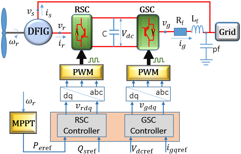
Figure 1. Overall system of the doubly-fed induction generator (DFIG) wind turbine.

2.1. Wind Turbine

In the generator-wind turbine system [14], the dynamic equation is written as:

$$\begin{array}{c}\hfill J{\omega }_r\left(t\right)\frac{d}{dt}{\omega }_r\left(t\right)=P_m\left(t\right)-P_e\left(t\right)\end{array}$$

(1)

where ${\omega }_r$ and $P_m$ are the rotor speed and mechanical power of the wind turbine, respectively; $P_e$ is the electrical power of the generator and J is the inertia of the generator-wind turbine system. The mechanical power is expressed by:

$$\begin{array}{ccc}\hfill P_m\left(t\right)& =& \frac{1}{2}\rho \pi R^2{C}_p(\lambda \left(t\right),\beta \left(t\right))V_w^3\left(t\right)\hfill \end{array}$$

(2)

where R is the blade size; ρ is the air density; $V_w$ is the wind speed; $C_p$ is the power coefficient; β is the pitch angle of the blade system and λ is the tip speed ratio defined by:

$$\begin{array}{ccc}\hfill \lambda \left(t\right)& =& \frac{R{\omega }_r\left(t\right)}{V_w\left(t\right)}\hfill \end{array}$$

(3)

The maximum mechanical power $P_{\max }$ is defined as:

$$\begin{array}{ccc}\hfill P_{\max }\left(t\right)& =& \frac{1}{2}\rho \pi R^2{C}_{p\max }\left(\beta \right)V_w^3\left(t\right)\hfill \end{array}$$

(4)

An example of $C_p(\lambda ,\beta )$ [18] and $P_m$ when $\beta =0$ is shown in Figure 2.

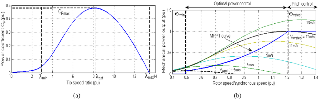
Figure 2. Characteristics of the wind turbine when $\beta =0$: (a) $C_p$ versus λ; (b) $P_{\max }$ versus ${\omega }_r$.

Figure 2a indicates that when $\beta =0$, there exists a maximum point $C_{p\max }:={max}_{\lambda }{C}_p(\lambda ,0)=0.48$ attained by ${\lambda }_{\mathrm{opt}}=8.123$. As can be seen in Figure 2b, the wind turbine works in the optimal power control region when the rotor speed is between the minimum speed ${\omega }_{r\min }$ and the rated speed ${\omega }_{r\mathrm{rated}}$ or when the wind speed is between the minimum speed $V_{w\min }$ and the rated speed $V_{w\mathrm{rated}}$. In this region, it is desirable for the wind turbine to operate on the locus of the maximum power point $P_{\max }$. This locus, named the MPPT-curve, is described by:

$$\begin{array}{ccc}\hfill P_{\mathrm{mppt}}\left(t\right)& =& k_{\mathrm{opt}}{\omega }_r^3\left(t\right)\hfill \end{array}$$

(5)

where:

$$k_{\mathrm{opt}}=\frac{1}{2}\rho \pi R^5\frac{C_{p\max }}{{\lambda }_{\mathrm{opt}}^3}$$

(6)

The objective of this paper is to propose an MPPT-scheme and a controller, such that the wind turbine operates on the MPPT curve as ${\omega }_{r\min }\le {\omega }_r\left(t\right)<{\omega }_{r\mathrm{rated}}$.

In fact, ${max}_{\lambda }{C}_p(\lambda ,\beta )$ is decreased when β increases [19], and ${max}_{\lambda }{C}_p(\lambda ,\beta )$ only reaches to ${max}_{\lambda ,\beta }{C}_p(\lambda ,\beta )$ at $\beta ={\beta }_{\min }$, where ${\beta }_{\min }$ is the minimum value of the pitch angle in its operation range and ${\beta }_{\min }$ is normally zero. In other words, to obtain ${max}_{\lambda ,\beta }{C}_p(\lambda ,\beta )$, the pitch angle β is normally set at ${\beta }_{\min }$. Hence, without loss of generality, the following assumption is used in this research.

Assumption 1. The pitch angle β is kept at ${\beta }_{\min }=0$ as ${\omega }_{r\min }\le {\omega }_r\left(t\right)<{\omega }_{r\mathrm{rated}}$.

2.2. DFIG

In the dqframe, the DFIG can be described as [19,20]:

$$\left\{\begin{array}{c}{v}_s\left(t\right)=R_s{i}_s\left(t\right)+L_s\frac{d}{dt}{i}_s\left(t\right)+L_m\frac{d}{dt}{i}_r\left(t\right)+{\omega }_s\Theta (L_s{i}_s\left(t\right)+L_m{i}_r\left(t\right))\hfill \\ v_r\left(t\right)=R_r{i}_r\left(t\right)+L_r\frac{d}{dt}{i}_r\left(t\right)+L_m\frac{d}{dt}{i}_s\left(t\right)+{\omega }_{s}s\left(t\right)\Theta (L_m{i}_s\left(t\right)+L_r{i}_r\left(t\right))\hfill \end{array}\right.$$

(7)

where $v_s={\left[\begin{array}{cc}{v}_{sd}& v_{sq}\end{array}\right]}^{\mathrm{T}}$ is the stator-side voltage; $v_r={\left[\begin{array}{cc}{v}_{rd}& v_{rq}\end{array}\right]}^{\mathrm{T}}$ is the rotor-side voltage; $i_s={\left[\begin{array}{cc}{i}_{sd}& i_{sq}\end{array}\right]}^{\mathrm{T}}$ is the stator-side current; $i_r={\left[\begin{array}{cc}{i}_{rd}& i_{rq}\end{array}\right]}^{\mathrm{T}}$ is the rotor-side current and $\Theta =\left[\begin{array}{cc}0& -1\\ 1& 0\end{array}\right]$. ω, R, L and s represent rotational speed, resistance, inductance and rotor slip, respectively; subscripts $r,s$ and m stand for rotor-side, stator-side and magnetization. Note that ${\omega }_s$ is normally constant. The rotor slip of the DFIG is defined by:

$$\begin{array}{c}\hfill s\left(t\right)=1-\frac{{\omega }_r\left(t\right)}{{\omega }_s}\end{array}$$

(8)

The power output of the generator is described by:

$$\begin{array}{c}\hfill P_e\left(t\right)=P_s\left(t\right)+P_r\left(t\right)=(1-s\left(t\right))P_s\left(t\right)=\frac{{\omega }_r\left(t\right)}{{\omega }_s}{P}_s\left(t\right)\end{array}$$

(9)

where $P_s$ and $P_r$ are the stator-side and rotor-side power, respectively.

Assumption 2. The stator flux is constant, and the d-axis of the dq-frame is oriented with the stator flux vector. Hence,

$$\begin{array}{c}\hfill {\Psi }_s\left(t\right)=\left[\begin{array}{c}{\Psi }_{sd}\left(t\right)\\ {\Psi }_{sq}\left(t\right)\end{array}\right]\equiv \left[\begin{array}{c}{\Psi }_{sd}\\ 0\end{array}\right]=L_s{i}_s\left(t\right)+L_m{i}_r\left(t\right)\end{array}$$

(10)

Then,

$$\begin{array}{c}\hfill L_s\frac{d}{dt}{i}_s\left(t\right)+L_m\frac{d}{dt}{i}_r\left(t\right)=0\end{array}$$

(11)

Moreover, the resistance of the stator winding can be ignored, i.e., $R_s=0$.

By substituting Equations (10) and (11) and $R_s=0$ into Equation (7), we have:

$$\begin{array}{ccc}\hfill v_s\left(t\right)& =& {\left[\begin{array}{cc}0& {\omega }_s{\Psi }_{sd}\end{array}\right]}^{\mathrm{T}}={\left[\begin{array}{cc}0& V_s\end{array}\right]}^{\mathrm{T}}\hfill \end{array}$$

(12)

because $V_s=\parallel v_s\left(t\right)\parallel$. From Equations (10) and (12), we have:

$$\begin{array}{ccc}& & L_s{i}_s\left(t\right)+L_m{i}_r\left(t\right)=\frac{1}{{\omega }_s}{\left[\begin{array}{cc}{V}_s& 0\end{array}\right]}^{\mathrm{T}}\hfill \end{array}$$

(13)

By substituting Equation (13) into the second part of Equation (7), we have:

$$\begin{array}{ccc}\hfill \frac{d}{dt}{i}_r\left(t\right)& =& A_1\left(t\right)i_r\left(t\right)+{\displaystyle \frac{1}{\sigma }}{v}_r\left(t\right)-d_1\left(t\right)\hfill \end{array}$$

(14)

where:

$$\begin{array}{ccc}\hfill \sigma & =& L_r-{\displaystyle \frac{L_m^2}{L_s}},{\tilde{V}}_s={\displaystyle \frac{L_m}{L_s}}{V}_s,\hfill \end{array}$$

(15)

$$\begin{array}{ccc}\hfill A_1\left(t\right)& =& -{\displaystyle \frac{1}{\sigma }}\left[\begin{array}{cc}{R}_r& -\sigma {\omega }_{s}s\left(t\right)\\ \sigma {\omega }_{s}s\left(t\right)& R_r\end{array}\right],d_1\left(t\right)={\displaystyle \frac{{\tilde{V}}_s}{\sigma }}s\left(t\right)\left[\begin{array}{c}0\\ 1\end{array}\right]\hfill \end{array}$$

(16)

Lemma 1. A state-space representation of the active power $P_s$ and the reactive power $Q_s$ on the stator side is given by:

$$\frac{d}{dt}{x}_1\left(t\right)=A_1\left(t\right)x_1\left(t\right)-{\displaystyle \frac{{\tilde{V}}_s}{\sigma }}{v}_r\left(t\right)+c_1\left(t\right)$$

(17)

where:

$$\begin{array}{c}\hfill x_1\left(t\right)=\left[\begin{array}{c}{Q}_s\left(t\right)\\ P_s\left(t\right)\end{array}\right],c_1\left(t\right)=-{\displaystyle \frac{A_1\left(t\right)}{L_s{\omega }_s}}\left[\begin{array}{c}{V}_s^2\\ 0\end{array}\right]+{\tilde{V}}_s{d}_1\left(t\right)={\displaystyle \frac{V_s^2}{\sigma L_s}}\left[\begin{array}{c}{\displaystyle \frac{R_r}{{\omega }_s}}\\ L_{r}s\left(t\right)\end{array}\right]\end{array}$$

(18)

In addition, under Assumption 2, a state-space representation of the DFIG (from Equation (7)) is described by:

$$\begin{array}{ccc}\hfill \frac{d}{dt}x\left(t\right)& =& A\left(t\right)x\left(t\right)+B\left(t\right)v_r\left(t\right)+d\left(t\right)\hfill \end{array}$$

(19)

where:

$$\begin{array}{ccc}\hfill x\left(t\right)& =& \left[\begin{array}{c}{Q}_s\left(t\right)\\ P_e\left(t\right)\end{array}\right]\hfill \end{array}$$

(20)

$$\begin{array}{ccc}\hfill A\left(t\right)& =& C{\left(t\right)}^{-1}\left(A_1\left(t\right)C\left(t\right)-\dot{C}\left(t\right)\right)=\left[\begin{array}{cc}-1-{\displaystyle \frac{R_r}{\sigma }}& {\displaystyle \frac{{\omega }_s^2}{{\omega }_r\left(t\right)}}s\left(t\right)\\ -{\omega }_r\left(t\right)s\left(t\right)& {\displaystyle \frac{\frac{d}{dt}{\omega }_r\left(t\right)-{\omega }_s{\displaystyle \frac{R_r}{\sigma }}}{{\omega }_r\left(t\right)}}\end{array}\right]\hfill \end{array}$$

(21)

$$\begin{array}{ccc}\hfill B\left(t\right)& =& -{\displaystyle \frac{{\tilde{V}}_s}{\sigma }}{C}^{-1}\left(t\right)C\left(t\right)=\left[\begin{array}{cc}1& 0\\ 0& {\displaystyle \frac{{\omega }_s}{{\omega }_r\left(t\right)}}\end{array}\right]\hfill \end{array}$$

(22)

$$\begin{array}{ccc}\hfill d\left(t\right)& =& C{\left(t\right)}^{-1}{c}_1\left(t\right)={\displaystyle \frac{V_s^2}{\sigma L_s{\omega }_s}}\left[\begin{array}{c}{R}_r\\ L_r{\omega }_r\left(t\right)s\left(t\right)\end{array}\right]\hfill \end{array}$$

(23)

Proof. The power in the stator side are given as [20]:

$$\begin{array}{c}\hfill x_1\left(t\right)=\left[\begin{array}{c}{Q}_s\left(t\right)\\ P_s\left(t\right)\end{array}\right]=\left[\begin{array}{cc}-i_{sq}\left(t\right)& i_{sd}\left(t\right)\\ i_{sd}\left(t\right)& i_{sq}\left(t\right)\end{array}\right]\left[\begin{array}{c}{v}_{sd}\left(t\right)\\ v_{sq}\left(t\right)\end{array}\right]\end{array}$$

(24)

By substituting Equations (12) and (13) into Equation (24), we have:

$$\begin{array}{c}\hfill x_1\left(t\right)=V_s{i}_s\left(t\right)=-{\tilde{V}}_s{i}_r\left(t\right)+\frac{1}{L_s{\omega }_s}\left[\begin{array}{c}{V}_s^2\\ 0\end{array}\right]\end{array}$$

(25)

Then, from Equations (25) and (14), (17) changes as follows:

$$\begin{array}{ccc}\hfill \frac{d}{dt}{x}_1\left(t\right)& =& -{\tilde{V}}_s\frac{d}{dt}{i}_r\left(t\right)=-A_1\left(t\right){\tilde{V}}_s{i}_r\left(t\right)-{\displaystyle \frac{{\tilde{V}}_s}{\sigma }}{v}_r\left(t\right)+{\tilde{V}}_s{d}_1\left(t\right)\hfill \end{array}$$

$$\begin{array}{ccc}& =& A_1\left(t\right)x_1\left(t\right)-{\displaystyle \frac{{\tilde{V}}_s}{\sigma }}{v}_r\left(t\right)-\frac{A_1\left(t\right)}{L_s{\omega }_s}\left[\begin{array}{c}{V}_s^2\\ 0\end{array}\right]+{\tilde{V}}_s{d}_1\left(t\right)\hfill \end{array}$$

By applying a transformation:

$$x_1\left(t\right)=C\left(t\right)x\left(t\right)$$

(26)

to Equation (17), we have:

$$\begin{array}{c}\hfill \frac{d}{dt}{x}_1\left(t\right)=\dot{C}\left(t\right)x\left(t\right)+C\left(t\right)\frac{d}{dt}x\left(t\right)=A_1\left(t\right)x_1\left(t\right)-{\displaystyle \frac{{\tilde{V}}_s}{\sigma }}{v}_r\left(t\right)+c_1\left(t\right)\end{array}$$

(27)

Hence, Equation (19) changes to be:

$$\begin{array}{c}\hfill \frac{d}{dt}x\left(t\right)=C{\left(t\right)}^{-1}\left(A_1\left(t\right)C\left(t\right)-\dot{C}\left(t\right)\right)x\left(t\right)-{\displaystyle \frac{{\tilde{V}}_s}{\sigma }}C{\left(t\right)}^{-1}{v}_r\left(t\right)+C{\left(t\right)}^{-1}{c}_1\left(t\right)\end{array}$$

(28)

Here, it is easy to check Equations (23) and (21) by using:

$$\dot{C}\left(t\right)=\left[\begin{array}{cc}1& 0\\ 0& -{\displaystyle \frac{{\omega }_s}{{\omega }_r{\left(t\right)}^2}}\frac{d}{dt}{\omega }_r\left(t\right)\end{array}\right]$$

(29)

☐

2.3. Converter

The overall converter system is shown in Figure 1, where the RSC and GSC are linked by a DC circuit [3,20]. This DC circuit, called the “DC link”, consists of a capacitor. Normally, the GSC is connected to the grid via a filter (represented by a resistor $R_f$, an inductor $L_f$ in series and a power factor correction pfin parallel) [20]. This $R_f{L}_f$ circuit can be described in the $dq$frame as:

$$\begin{array}{c}\hfill v_g\left(t\right)=v_s\left(t\right)+R_f{i}_g\left(t\right)+L_f\frac{d}{dt}{i}_g\left(t\right)+L_f{\omega }_s\Theta i_g\left(t\right)\end{array}$$

(30)

where $v_g={\left[\begin{array}{cc}{v}_{gd}& v_{gq}\end{array}\right]}^{\mathrm{T}}$ is the voltage output of the GSC; $i_g={\left[\begin{array}{cc}{i}_{gd}& i_{gq}\end{array}\right]}^{\mathrm{T}}$ is the current output of the GSC and $R_f$ and $L_f$ are the resistance and inductance, respectively, of the $R_f{L}_f$ circuit.

Assumption 3. Power loss in converters and the $R_f{L}_f$ circuit is neglected [19,21].

Under Assumption 3, the DC link is described as [21]:

$$\begin{array}{c}\hfill \frac{d}{dt}{V}_{dc}\left(t\right)=\frac{1}{C{V}_{dc}\left(t\right)}\left(P_r\left(t\right)-P_g\left(t\right)\right)\end{array}$$

(31)

where C is the capacitance of the capacitor; $V_{dc}$ is the DC voltage on the DC link and $P_g$ is the active power output of the GSC [20].

Assumption 4. The $dq$ frame in which the d axis is oriented with the voltage vector $v_s$, so $v_{sd}\left(t\right)=V_s$ and $v_{sq}\left(t\right)=0$.

Under Assumption 4, the active power output of the GSC connected to the grid is described by:

$$\begin{array}{c}\hfill P_g\left(t\right)=v_{sd}\left(t\right)i_{gd}\left(t\right)+v_{sq}\left(t\right)i_{gq}\left(t\right)=V_s{i}_{gd}\left(t\right)\end{array}$$

(32)

Lemma 2. Under Assumption 4, a state-space representation of the GSC connected to the grid is described as:

$$\begin{array}{ccc}\hfill \frac{d}{dt}{i}_g\left(t\right)& =& A_2{i}_g\left(t\right)+{\displaystyle \frac{1}{L_f}}{v}_g\left(t\right)-{\displaystyle \frac{1}{L_f}}\left[\begin{array}{c}{V}_s\\ 0\end{array}\right]\hfill \end{array}$$

(33)

$$\begin{array}{ccc}\hfill A_2& =& -{\displaystyle \frac{R_f}{L_f}}I-{\omega }_s\Theta \hfill \end{array}$$

(34)

where I is the identity matrix.

Proof. From Equation (30), it is easy to obtain:

$$\begin{array}{c}\hfill \frac{d}{dt}{i}_g\left(t\right)=-\left({\displaystyle \frac{R_f}{L_f}}I+{\omega }_s\Theta \right)i_g\left(t\right)+{\displaystyle \frac{v_g\left(t\right)-v_s\left(t\right)}{L_f}}\end{array}$$

(35)

From Assumption 4, we have Equation (33). This completes the proof. ☐

3. Controller Design and Maximum Power Strategy

Assumption 5. We can measure $i_r$, $i_s$, $i_g$, $v_s$, $V_{dc}$ and ${\omega }_r$. In addition, we can manipulate $v_{rd}$, $v_{rq}$, $v_{gd}$ and $v_{gq}$ and know parameters $R_s,R_r,L_s,L_r$ and $L_m$.

Assumption 6. The $dq/abc$ transformation block, the PWM and the IGBT-valves in converters operate properly.

3.1. Rotor-Side Control

The objective of RSC is to maintain, at the desired references, the reactive power in the stator side $Q_s$ and the total active power output $P_e$ of the DFIG.

$$\begin{array}{c}\hfill x_{\mathrm{r}}^{\mathrm{T}}={\left[\begin{array}{cc}{Q}_{s\mathrm{ref}}& P_{e\mathrm{ref}}\end{array}\right]}^{\mathrm{T}}\end{array}$$

(36)

From Equations (9), (14) and (25), to adjust $Q_s$ and $P_e$ corresponding to $i_{rd}$ and $i_{rq}$, $v_{rd}$ and $v_{rq}$ must be regulated, respectively. To perform this task, previous studies employed PI controllers [9,22]. In this study, a new control law is proposed.

Lemma 3. (RSC control) Under Assumptions 2 and 5, when we can measure $\frac{d}{dt}{\omega }_r\left(t\right)$ for any desired reference $x_{\mathrm{r}}$ (from Equation (36)), if we use any positive definite matrix P,

$$\begin{array}{ccc}\hfill v_r\left(t\right)& =& -B{\left(t\right)}^{-1}\left(A\left(t\right)x\left(t\right)+P{e}_x\left(t\right)-\frac{d}{dt}{x}_{\mathrm{r}}\left(t\right)+d\left(t\right)\right)\hfill \end{array}$$

(37)

$$\begin{array}{ccc}\hfill e_x\left(t\right)& =& x_r\left(t\right)-x\left(t\right)\hfill \end{array}$$

(38)

for the DFIG (from Equation (19)), then it is ensured that:

$$\underset{t\to \infty }{lim}{e}_x\left(t\right)=0$$

(39)

Proof. By applying Equations (37) to (19), we have:

$$\begin{array}{ccc}\hfill \frac{d}{dt}x\left(t\right)& =& -P{e}_x\left(t\right)+\frac{d}{dt}{x}_{\mathrm{r}}\left(t\right)\hfill \end{array}$$

(40)

which is equivalent to:

$$\begin{array}{c}\hfill \frac{d}{dt}{e}_x\left(t\right)=-P{e}_x\left(t\right)\end{array}$$

(41)

It is obvious that when we define a Lyapunov function $V\left(e_x\right)=e_x^{\mathrm{T}}{e}_x$, its time derivative becomes:

$$\begin{array}{ccc}\hfill \frac{d}{dt}V\left(e_x\right)& =& 2e_x{\left(t\right)}^{\mathrm{T}}\frac{d}{dt}{e}_x\left(t\right)=-2e_x{\left(t\right)}^{\mathrm{T}}P{e}_x\left(t\right)<0\hfill \end{array}$$

(42)

for any $e_x\left(t\right)\ne 0$. Hence, $e_x\left(t\right)$ converges to zero. ☐

From Lemma 3, if the rotor voltage $v_r$ is designed as Equation (37), the power output of DFIG will converge to its reference value (given Equation (36)).

3.2. Maximum Output Power Control

The main objective of this section is to propose a new MPPT scheme that improves the conventional MPPT-curve method [22] so that $P_m$ approaches the neighbor of $P_{\max }$ as ${\omega }_{r\min }\le {\omega }_r\left(t\right)<{\omega }_{r\mathrm{rated}}$, as shown in Figure 2b. From Equation (4) and Figure 2a, $P_m\left(t\right)$ only reaches the neighbor of $P_{\max }$ as λ approaches the neighbor of ${\lambda }_{\mathrm{opt}}$. Therefore, in this study, a new strategy is proposed, such that λ approaches the neighbor of ${\lambda }_{\mathrm{opt}}$.

Assumption 7. The wind turbine operates in the optimal power control region, as shown in Figure 2b, and ${\lambda }_{\min }\le \lambda \left(t\right)\le {\lambda }_{\max }$, where ${\lambda }_{\min }={\displaystyle \frac{R{\omega }_{r\min }}{V_{w\mathrm{rated}}}}$. In addition, there exists a constant γ, such that $\left|\frac{d}{dt}{V}_w\left(t\right)\right|\le \gamma$.

For the wind turbine (from Equations (1)–(4)) and $C_p\left(\lambda \right)$ (shown in Section 4), we have Remark 1, as follows.

Remark 1. From (1) and (3) and from the definition of $k_{\mathrm{opt}}$, we have:

$$\begin{array}{c}\hfill P_m\left(t\right)-k_{\mathrm{opt}}{\omega }_r^3\left(t\right)=\frac{\rho \pi R^5{\omega }_r^3\left(t\right)}{2}\left(\frac{C_p\left(\lambda \left(t\right)\right)}{{\lambda }^3\left(t\right)}-\frac{C_{p\max }}{{\lambda }_{\mathrm{opt}}^3}\right)=-\zeta \left(t\right)\left(\lambda \left(t\right)-{\lambda }_{\mathrm{opt}}\right)\end{array}$$

(43)

where:

$$\begin{array}{c}\hfill \zeta \left(t\right)=\frac{\rho \pi R^5}{2{\lambda }_{\mathrm{opt}}^3}\frac{{\omega }_r^3\left(t\right)}{\lambda \left(t\right)-{\lambda }_{\mathrm{opt}}}\left(C_{p\max }-C_p\left(\lambda \left(t\right)\right)\frac{{\lambda }_{\mathrm{opt}}^3}{{\lambda }^3\left(t\right)}\right)\end{array}$$

(44)

is positive, continuous and bounded in ${\lambda }_{\min }\le \lambda \left(t\right)\le {\lambda }_{\max }$.

Theorem 1. Under Assumption 7, suppose that we use a positive constant $\alpha <J$, $k_{\mathrm{opt}}$ (given in Equation (6)), and $P_{e\mathrm{ref}}$ (given in Equation (36)) for the RSC control (given in (37)) as:

$$\begin{array}{ccc}\hfill P_{e\mathrm{ref}}\left(t\right)& =& k_{\mathrm{opt}}{\omega }_r^3\left(t\right)-\alpha {\omega }_r\left(t\right)\frac{d}{dt}{\omega }_r\left(t\right)\hfill \end{array}$$

(45)

If there exists a positive constant $0<\chi <2\zeta \left(t\right)$, such that:

$$\begin{array}{c}\hfill \tilde{P}:=2P-\left[\begin{array}{cc}0& 0\\ 0& {\chi }^{-1}{\displaystyle \frac{\lambda \left(t\right)}{\eta {\omega }_r^2\left(t\right)}}\end{array}\right]>0\end{array}$$

(46)

for the definite matrix $P>0$ in Equation (37) and all t, then there exists a time $t_0>0$, such that for $e_{\lambda }\left(t\right)=\lambda \left(t\right)-{\lambda }_{\mathrm{opt}}$,

$$\begin{array}{c}\hfill \left|e_{\lambda }\left(t\right)\right|\le 2(J-\alpha )\gamma max\frac{{\omega }_r^2\left(t\right)}{(2\zeta \left(t\right)-\chi )V_w\left(t\right)}\end{array}$$

(47)

for all $t\ge t_0$.

Proof. First, let $e_x\left(t\right)={\left[\begin{array}{cc}{e}_Q& e_P\end{array}\right]}^{\mathrm{T}}=x_{\mathrm{r}}\left(t\right)-x\left(t\right)$. We define a Lyapunov candidate as:

$$\begin{array}{c}\hfill V(e_x,e_{\lambda })=e_x{\left(t\right)}^{\mathrm{T}}{e}_x\left(t\right)+e_{\lambda }^2\left(t\right)\end{array}$$

(48)

The time derivative of the Lyapunov function is:

$$\begin{array}{ccc}\hfill \dot{V}(e_x,e_{\lambda })& =& 2e_x{\left(t\right)}^{\mathrm{T}}\frac{d}{dt}{e}_x\left(t\right)+2e_{\lambda }\left(t\right)\frac{d}{dt}\lambda \left(t\right)\hfill \end{array}$$

(49)

Since $\lambda \left(t\right)=R{\omega }_r\left(t\right)/V_w\left(t\right)$, we have:

$$\begin{array}{ccc}\hfill \frac{d}{dt}\lambda \left(t\right)& =& {\displaystyle \frac{\lambda \left(t\right)}{{\omega }_r\left(t\right)}}\frac{d}{dt}{\omega }_r\left(t\right)-{\displaystyle \frac{\lambda \left(t\right)}{V_w\left(t\right)}}\frac{d}{dt}{V}_w\left(t\right)\hfill \end{array}$$

(50)

From Equation (1) and $e_P\left(t\right)=P_{e\mathrm{ref}}\left(t\right)-P_e\left(t\right)$, we have:

$$\begin{array}{ccc}\hfill \frac{d}{dt}{\omega }_r\left(t\right)& =& \frac{1}{J{\omega }_r\left(t\right)}(P_m\left(t\right)+e_P\left(t\right)-P_{e\mathrm{ref}}\left(t\right))\hfill \end{array}$$

(51)

By substituting $P_{e\mathrm{ref}}$ from Equations (45) into (51), we get:

$$\begin{array}{ccc}\hfill \frac{d}{dt}{\omega }_r\left(t\right)& =& \frac{1}{\eta {\omega }_r\left(t\right)}(P_m\left(t\right)-k_{\mathrm{opt}}{\omega }_r^3\left(t\right)+e_P\left(t\right))\hfill \end{array}$$

(52)

where $\eta =J-\alpha >0$. By substituting Equations (43) into (52), we have:

$$\begin{array}{ccc}\hfill \frac{d}{dt}{\omega }_r\left(t\right)& =& \frac{1}{\eta {\omega }_r\left(t\right)}\left(e_P\left(t\right)-\zeta \left(t\right)e_{\lambda }\left(t\right)\right)\hfill \end{array}$$

(53)

From Equations (53) and (50), we have:

$$\begin{array}{c}\hfill 2e_{\lambda }\left(t\right)\frac{d}{dt}\lambda \left(t\right)={\delta }_1\left(t\right)\left(2e_P\left(t\right)e_{\lambda }\left(t\right)-2\zeta \left(t\right)e_{\lambda }^2\left(t\right)\right)-{\displaystyle \frac{2\lambda \left(t\right)}{V_w\left(t\right)}}{e}_{\lambda }\left(t\right)\frac{d}{dt}{V}_w\left(t\right)\end{array}$$

(54)

where ${\delta }_1\left(t\right):={\displaystyle \frac{\lambda \left(t\right)}{\eta {\omega }_r^2\left(t\right)}}>0$. Since:

$$\begin{array}{ccc}\hfill 2e_P\left(t\right)e_{\lambda }\left(t\right)& \le & {\chi }^{-1}{e}_P^2\left(t\right)+\chi e_{\lambda }^2\left(t\right)\hfill \end{array}$$

(55)

$$\begin{array}{ccc}\hfill \left|\frac{d}{dt}{V}_w\left(t\right)\right|& \le & \gamma \hfill \end{array}$$

(56)

$$\begin{array}{ccc}\hfill -\frac{2\lambda \left(t\right)e_{\lambda }\left(t\right)}{V_w\left(t\right)}\frac{d}{dt}{V}_w\left(t\right)& \le & \frac{2\lambda \left(t\right)|e_{\lambda }\left(t\right)|}{V_w\left(t\right)}\gamma \hfill \end{array}$$

(57)

we have:

$$\begin{array}{c}\hfill 2e_{\lambda }\left(t\right)\frac{d}{dt}\lambda \left(t\right)\le {\chi }^{-1}{\delta }_1\left(t\right)e_P^2\left(t\right)-{\delta }_2\left(t\right)e_{\lambda }^2\left(t\right)+{\delta }_3\left(t\right)\left|e_{\lambda }\left(t\right)\right|\end{array}$$

(58)

where:

$${\delta }_2\left(t\right):=(2\zeta \left(t\right)-\chi ){\delta }_1\left(t\right)>0$$

and:

$${\delta }_3\left(t\right):=\frac{2\lambda \left(t\right)\gamma }{V_w\left(t\right)}\ge 0$$

From Equations (42) and (58), (49) becomes:

$$\begin{array}{c}\hfill \dot{V}(e_x,e_{\lambda })\le -2e_x^{\mathrm{T}}\left(t\right)P{e}_x\left(t\right)+{\chi }^{-1}{\delta }_1\left(t\right)e_P^2\left(t\right)-{\delta }_2\left(t\right)e_{\lambda }^2\left(t\right)+{\delta }_3\left(t\right)\left|e_{\lambda }\left(t\right)\right|\end{array}$$

(59)

Obviously,

$$\begin{array}{c}\hfill -2e_x^{\mathrm{T}}\left(t\right)P{e}_x\left(t\right)+{\chi }^{-1}{\delta }_1\left(t\right)e_P^2\left(t\right)=-e_x^{\mathrm{T}}\left(t\right)\tilde{P}{e}_x\left(t\right)<0\end{array}$$

Hence,

$$\begin{array}{c}\hfill \dot{V}(e_x,e_{\lambda })\le -{\delta }_2\left(t\right)|e_{\lambda }\left(t\right)|\left(|e_{\lambda }\left(t\right)|-\frac{{\delta }_3\left(t\right)}{{\delta }_2\left(t\right)}\right)\le -{\delta }_2\left(t\right)\left|e_{\lambda }\left(t\right)\right|\left(|e_{\lambda }\left(t\right)|-{\Delta }_3\right)\end{array}$$

(60)

where:

$$\begin{array}{c}\hfill {\Delta }_3=max\frac{{\delta }_3\left(t\right)}{{\delta }_2\left(t\right)}=2\eta \gamma max\frac{{\omega }_r^2\left(t\right)}{(2\zeta \left(t\right)-\chi )V_w\left(t\right)}\end{array}$$

(61)

Then, $V(e_x,e_{\lambda })$ decreases when:

$$|e_{\lambda }\left(t\right)|>{\Delta }_3=2\eta \gamma max\frac{{\omega }_r^2\left(t\right)}{(2\zeta \left(t\right)-\chi )V_w\left(t\right)}$$

(62)

This completes the proof of Theorem 1. ☐

From Theorem Equation (1), if the reference power $P_{e\mathrm{ref}}$ in Equation (36) is calculated as Equation (45), the tip-speed ratio λ of the wind turbine will converge to the neighbor of ${\lambda }_{\mathrm{opt}}$ and, hence, $P_m$ will approach its maximum value.

3.3. Grid-Side Control

From Equation (3), if $V_{dc}$ on the DC link is kept at a constant value, all power output generating in the rotor side will be delivered to the connected grid. Moreover, if the $i_{gq}-$ component is maintained at zero, the power loss in the $R_f{L}_f$ circuit will be minimized. Consequently, the conversion energy efficiency of the DFIG-wind turbine will be maximized. Without loss of generality, in this section, the objective of GSC is to maintain $V_{dc}\left(t\right)$ and $i_{gq}\left(t\right)$ at desired references $V_{dc\mathrm{ref}}\left(t\right)$ and $i_{gq\mathrm{ref}}\left(t\right)$, respectively. From Equations (31)–(33), we need to adjust $v_g$.

Theorem 2. For any desired reference $V_{dc\mathrm{ref}}\left(t\right)$ and $i_{gq\mathrm{ref}}\left(t\right)$, for GSC (given in Equation (33)), we use:

$$\begin{array}{ccc}\hfill v_g\left(t\right)& =& L_f\left(\frac{d}{dt}{i}_{gr}\left(t\right)+Q\left(t\right)e_i\left(t\right)-A_2{i}_g\left(t\right)\right)+\left[\begin{array}{c}{V}_s\\ 0\end{array}\right]\hfill \end{array}$$

(63)

$$\begin{array}{ccc}\hfill i_{gr}\left(t\right)& =& \left[\begin{array}{c}{\displaystyle \frac{1}{V_s}}\left(P_r\left(t\right)-C{V}_{dc}\left(t\right)\frac{d}{dt}{V}_{dc\mathrm{ref}}\left(t\right)\right)-k{e}_v\left(t\right)\\ i_{gq\mathrm{ref}}\left(t\right)\end{array}\right]\hfill \end{array}$$

(64)

$$\begin{array}{ccc}\hfill e_v\left(t\right)& =& V_{dc\mathrm{ref}}\left(t\right)-V_{dc}\left(t\right)\hfill \end{array}$$

(65)

$$\begin{array}{ccc}\hfill e_i\left(t\right)& =& i_{gr}\left(t\right)-i_g\left(t\right)\hfill \end{array}$$

(66)

and if there exists a constant $k>1/2$ and a positive definite matrix $Q\left(t\right)$, such that:

$$\begin{array}{c}\hfill Q\left(t\right)-\frac{1}{V_{dc}\left(t\right)}\left[\begin{array}{cc}1& 0\\ 0& 0\end{array}\right]>0\end{array}$$

(67)

it is ensured that:

$$\underset{t\to \infty }{lim}{e}_v\left(t\right)=0\text{and}\underset{t\to \infty }{lim}\left(i_{gq\mathrm{ref}}\left(t\right)-i_{gq}\left(t\right)\right)=0$$

Proof. By substituting Equations (63) into (33), we have:

$$\begin{array}{ccc}\hfill \frac{d}{dt}{i}_g\left(t\right)& =& \frac{d}{dt}{i}_{gr}\left(t\right)+Q\left(t\right)\left(i_{gr}\left(t\right)-i_g\left(t\right)\right)\hfill \end{array}$$

(68)

By defining $e_i\left(t\right)={\left[\begin{array}{cc}{e}_{i1}\left(t\right)& e_{i2}\left(t\right)\end{array}\right]}^{\mathrm{T}}=i_{gr}\left(t\right)-i_g\left(t\right)$, Equation (68) means:

$$\begin{array}{ccc}\hfill \frac{d}{dt}{e}_i\left(t\right)& =& -Q\left(t\right)e_i\left(t\right)\hfill \end{array}$$

(69)

Furthermore, by defining $e_v\left(t\right)=V_{dc\mathrm{ref}}\left(t\right)-V_{dc}\left(t\right)$, from Equation (31), we have:

$$\begin{array}{ccc}\hfill \frac{d}{dt}{e}_v\left(t\right)& =& \frac{d}{dt}{V}_{dc\mathrm{ref}}\left(t\right)-\frac{1}{C{V}_{dc}\left(t\right)}\left(P_r\left(t\right)-V_s{i}_{gd}\left(t\right)\right)\hfill \end{array}$$

(70)

where we use $P_g\left(t\right)=V_s{i}_{gd}\left(t\right)$. To use Equation (70), we can show:

$$\begin{array}{ccc}\hfill e_{i1}\left(t\right)& =& -\frac{C{V}_{dc}\left(t\right)}{V_s}\frac{d}{dt}{e}_v\left(t\right)-k{e}_v\left(t\right)\hfill \end{array}$$

(71)

When we introduce a Lyapunov function:

$$\begin{array}{ccc}\hfill V(e_v,e_i)& =& \frac{C}{V_s}{e}_v^2\left(t\right)+\frac{1}{2}{e}_i^{\mathrm{T}}\left(t\right)e_i\left(t\right)\hfill \end{array}$$

(72)

and its time derivative is expressed as:

$$\begin{array}{ccc}\hfill \dot{V}(e_v,e_i)& =& \frac{2C}{V_s}{e}_v\left(t\right)\frac{d}{dt}{e}_v\left(t\right)+e^{\mathrm{T}}\left(t\right)\frac{d}{dt}{e}_i\left(t\right)=-\frac{2}{V_{dc}\left(t\right)}{e}_v\left(t\right)\left(e_5\left(t\right)+k{e}_v\left(t\right)\right)-e_i^{\mathrm{T}}\left(t\right)Q\left(t\right)e_i\left(t\right)\hfill \end{array}$$

$$\begin{array}{ccc}& =& -\frac{2k-1}{V_{dc}\left(t\right)}{e}_v^2\left(t\right)-\frac{1}{V_{dc}\left(t\right)}{\left(e_v\left(t\right)+e_{i1}\left(t\right)\right)}^2+\frac{1}{V_{dc}\left(t\right)}{e}_{i1}^2\left(t\right)-e_i^{\mathrm{T}}\left(t\right)Q\left(t\right)e_i\left(t\right)\hfill \end{array}$$

Hence, if Equation (67) holds, then $\dot{V}(e_v,e_i)<0$ for all nonzero $e_v$ and $e_i$. This completes the proof of Theorem 2. ☐

From Theorem 2, if $v_g$ is designed as Equation (63), where $V_{dc\mathrm{ref}}$ and $i_{gq\mathrm{ref}}$ are set at a constant and zero, respectively, the power loss in the converter and $R_f{L}_f$ will be minimized.

Control diagrams for the RSC and GSC are indicated in Figure 3.

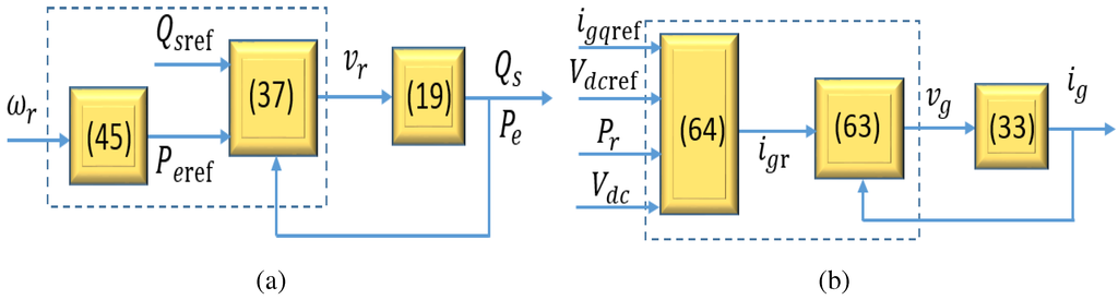
Figure 3. Control of DFIG: (a) rotor-side converter (RSC) controller; (b) grid side-converter (GSC) controller.

4. Performance Validation

This section compares the simulation results of the 1.5-MW DFIG wind turbine using the proposed MPPT scheme with that of the same wind turbine using the conventional MPPT-curve method using PI control [9,22]. MATLAB/Simulink was used for the simulation. The parameters used for the wind turbine in the simulation are given in Table 1 [23].

Table 1. Parameters of the wind turbine.

Name	Symbol	Value	Unit
The length of blade	R	35.25	m
Rated rotor speed	${\omega }_{r\mathrm{rated}}$	22	rpm
Minimum rotor speed	${\omega }_{r\min }$	11	rpm
Rated wind speed	$V_{w\mathrm{rated}}$	12	m/s

Table 1. Parameters of the wind turbine.

Name	Symbol	Value	Unit
The length of blade	R	35.25	m
Rated rotor speed	${\omega }_{r\mathrm{rated}}$	22	rpm
Minimum rotor speed	${\omega }_{r\min }$	11	rpm
Rated wind speed	$V_{w\mathrm{rated}}$	12	m/s

The power coefficient of the wind turbine [18] is:

$$\begin{array}{ccc}\hfill C_p(\lambda ,\beta )& =& 0.5176\left({\displaystyle \frac{116}{{\lambda }_i}}-0.4\beta -5\right)e^{-{\displaystyle \frac{21}{{\lambda }_i}}}+0.0068\lambda \hfill \end{array}$$

where:

$$\begin{array}{ccc}\hfill \frac{1}{{\lambda }_i}& =& \frac{1}{\lambda +0.08\beta }-\frac{0.035}{{\beta }^3+1}\hfill \end{array}$$

with air density $\rho =1.1225$$\mathrm{kg}/{\mathrm{m}}^3$ [20] and system inertia $J\approx 4.45\times {10}^5$$\mathrm{kg}·{\mathrm{m}}^2$ [17]. A wind speed profile (shown in Figure 4) was used, in which $\frac{d}{dt}{V}_w\left(t\right)\le \gamma =0.44$$\mathrm{m}/{\mathrm{s}}^2$. To test the proposed MPPT strategy and controllers, the wind velocity was always below the rated wind speed, 12 m/s.

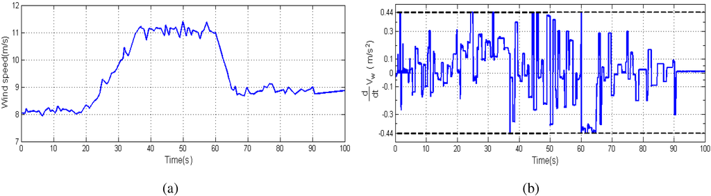
Figure 4. Wind speed profile: (a) $V_w\left(t\right)$ and (b)$\frac{d}{dt}{V}_w\left(t\right)$.

The rated rotor speed and the minimum one are ${\omega }_{r\mathrm{rated}}=2.3$$\mathrm{rad}/\mathrm{s}$ and ${\omega }_{r\min }=1.15$$\mathrm{rad}/\mathrm{s}$, respectively. From the $C_p(\lambda ,\beta )$ equation and $\beta =0$, we can obtain ${\lambda }_{\mathrm{opt}}=8.123$ and ${\lambda }_{\max }=13.4$. The minimum value of λ is defined by:

$$\begin{array}{ccc}\hfill {\lambda }_{\min }& =& \frac{R{\omega }_{r\min }}{V_{w\mathrm{rated}}}=\frac{35.25\times 1.15}{12}=3.4,\text{and}{V}_{w\min }=\frac{R{\omega }_{r\min }}{{\lambda }_{\mathrm{opt}}}=\frac{35.25\times 1.15}{8.123}=5\mathrm{m}/\mathrm{s}\hfill \end{array}$$

The reference values settings for the RSC and GSC control (from (37) and Equations (63)), with $Q_{s\mathrm{ref}}\left(t\right)=0$, $V_{dc\mathrm{ref}}$ = 1150 $\mathrm{V}$ and $i_{gq\mathrm{ref}}\left(t\right)=0$, are:

$$P=\left[\begin{array}{cc}2& 0\\ 0& 2\end{array}\right],Q\left(t\right)=\left[\begin{array}{cc}0.4+{\displaystyle \frac{1}{V_{dc}\left(t\right)}}& 0\\ 0& 1.05\end{array}\right]\text{and}k=30$$

We used $P_{e\mathrm{ref}}$ for the RSC control (from Equation (45)) with $\alpha =0.3$J and $k_{\mathrm{opt}}=0.85\times {10}^5$$\mathrm{kg}·{\mathrm{m}}^2$.

We have:

$$\begin{array}{c}\hfill max{\delta }_1\left(t\right)={\displaystyle \frac{{\lambda }_{\max }}{\eta {\omega }_{r\min }^2}}=\frac{13.4}{3.12\times {10}^5\times 1.{15}^2}\approx 0\end{array}$$

(73)

where $\eta =J-\alpha =0.7$$J=3.12\times {10}^5$$\mathrm{kg}·{\mathrm{m}}^2$. With 5 $\mathrm{m}/\mathrm{s}\le V_w\left(t\right)\le 12$$\mathrm{m}/\mathrm{s}$ and $1.15$$\mathrm{rad}/\mathrm{s}\le {\omega }_r\left(t\right)\le 2.3$$\mathrm{rad}/\mathrm{s}$, ζ versus ${\omega }_r$ and $V_w$ are shown in Figure 5a.

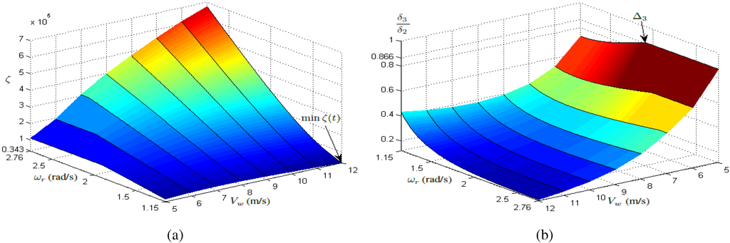
Figure 5. (a) ζ and (b) $\frac{{\delta }_3}{{\delta }_2}$ versus ${\omega }_r$ and $V_w$.

From Figure 5a, we can obtain $min\zeta \left(t\right)=0.343\times {10}^5$; we choose $\chi =1$. With $\chi =1$, $\frac{{\delta }_3}{{\delta }_2}$ versus ${\omega }_r$ and $V_w$ are shown in Figure 5b. From that figure, we obtain ${\Delta }_3=0.866$. Obviously, the condition in Equation (46) is satisfied, and Equation (47) gives the bound of the tip-speed ratio λ as:

$$\begin{array}{ccc}\hfill \left|\lambda \left(t\right)-{\lambda }_{\mathrm{opt}}\right|& \le & {\Delta }_3=0.866\hfill \end{array}$$

Hence, $7.257\le \lambda \left(t\right)\le 9.989$.

We compare the efficiency of the maximum power output in Figure 6. In Figure 6a, the power coefficient $C_p$ is always maintained at its maximum value $C_{p\max }=0.48$ when the wind speed varies insignificantly. However, deterioration of $C_p$ during a period of rapid change in wind conditions still occurs. Due to the large inertia of the system when the wind velocity increases or decreases quickly, the rotor speed of the turbine cannot respond instantaneously. The tip-speed ratio λ cannot keep its optimum value ${\lambda }_{\mathrm{opt}}$; and hence, the decrease in $C_p$ is unavoidable. Compared to the conventional MPPT-curve method, in the proposed method, $C_p$ retains $C_{p\max }$ promptly, mainly because its inertia seems to be reduced from J to $J-\alpha$; thus, λ retains ${\lambda }_{\mathrm{opt}}$. When the MPPT-curve method is used, the minimum value of $C_p$ during the interval of rapid decrease in wind speed is 0.45; when the proposed method is used, that value is 0.472.

Figure 6b depicts that, with the proposed scheme, λ only varies in a narrow range, $7.257<\lambda \left(t\right)<8.989$, which is theoretically ensured by Theorem 1. By contrast, with the conventional scheme, λ vacillates in a larger range.

Concerning mechanical power, Figure 6c depicts the error between $P_{\max }$ and $P_m$. Obviously, during periods of stable wind conditions, there is no difference between the conventional and proposed methods. However, when the wind velocity dramatically varies, the error in the proposed method is significantly smaller than that in the other, mainly because the power coefficient $C_p$, with the conventional method, is reduced significantly during sudden variations in wind conditions.

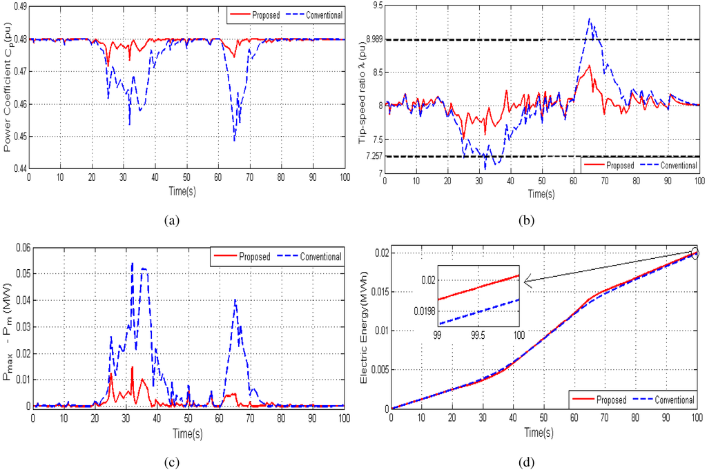
Figure 6. Simulation results using the proposed maximum mechanical power method: (a) power coefficient; (b) operation range of λ; (c) error between $P_{\max }$ and $P_m$; (d) electrical energy output.

Figure 6d indicates that during the period of increasing wind velocity [20 s,40 s], a higher mechanical energy part is stored in its mechanical system to accelerate the rotor speed by the proposed method than that by the conventional MPPT-curve method. Hence, the electrical energy output in this period is smaller. However, this mechanical energy part is released during deceleration of the rotor speed, as seen in [60 s,75 s]. Obviously, by the proposed method, the total electrical energy output of the generator is higher than that by the conventional one, as shown in Figure 6d, mainly because $P_m$, in the proposed method, has a higher value. This affirms the improved efficiency of the proposed method.

MPPT tracking ability is indicated in Figure 7 where the wind speed profile shown in Figure 4a is used. As that figure shows, with the proposed method, the curve $P_m$ versus $V_w$ is approximate to the ideal curve, $P_{\max }$ versus $V_w$, while, with the conventional scheme, this is impossible (see Figure 7b). In other words, the wind turbine with the proposed method can track the MPPT better than that with the conventional one.

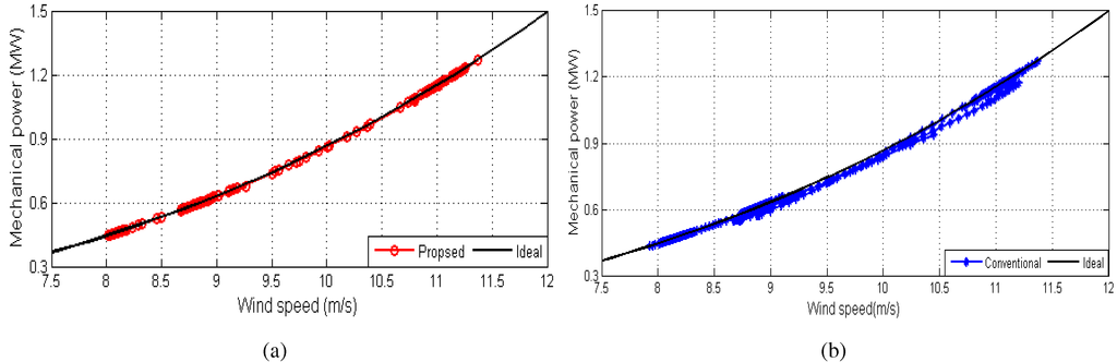
Figure 7. $P_m\left(t\right)$ versus $V_w\left(t\right)$: (a) proposed scheme and (b) conventional MPPT-curve method.

Concerning the proposed control laws and scheme, Figure 8a argues that both $e_Q\left(t\right)=Q_{s\mathrm{ref}}\left(t\right)-Q_s\left(t\right)$ and $e_P\left(t\right)=P_{e\mathrm{ref}}\left(t\right)-P_e\left(t\right)$ are approximately zero, which means that $Q_s$ and $P_e$ always converge to their reference values, $Q_{s\mathrm{ref}}$ and $P_{e\mathrm{ref}}$, respectively; in other words, Lemma 3 is ensured. Likely, Theorem 2 is also guaranteed from Figure 8b because $e_v\left(t\right)=V_{dc\mathrm{ref}}\left(t\right)-V_{dc}\left(t\right)$ and $e_{i2}\left(t\right)=i_{gq\mathrm{ref}}\left(t\right)-i_{gq}\left(t\right)$ are very small. In other words, the controllers suggested for the RSC and GSC have good performance.

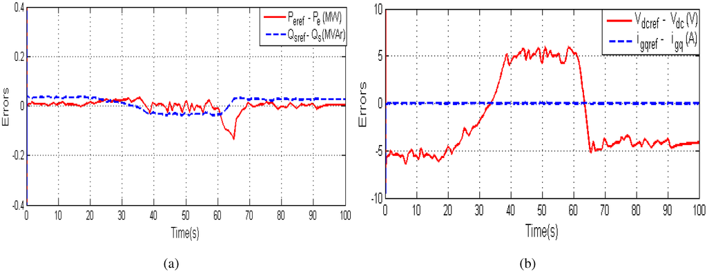
Figure 8. Error between reference signal and actual output in the controller: (a) RSC (b) GSC.

When a rapid wind profile as shown in Figure 9a is used, the simulation results are demonstrated in Figure 9b–Figure 9d. Obviously, the wind turbine by the proposed method has better performance in the power coefficient $C_p$, the mechanical power and the electrical energy output than by the conventional one.

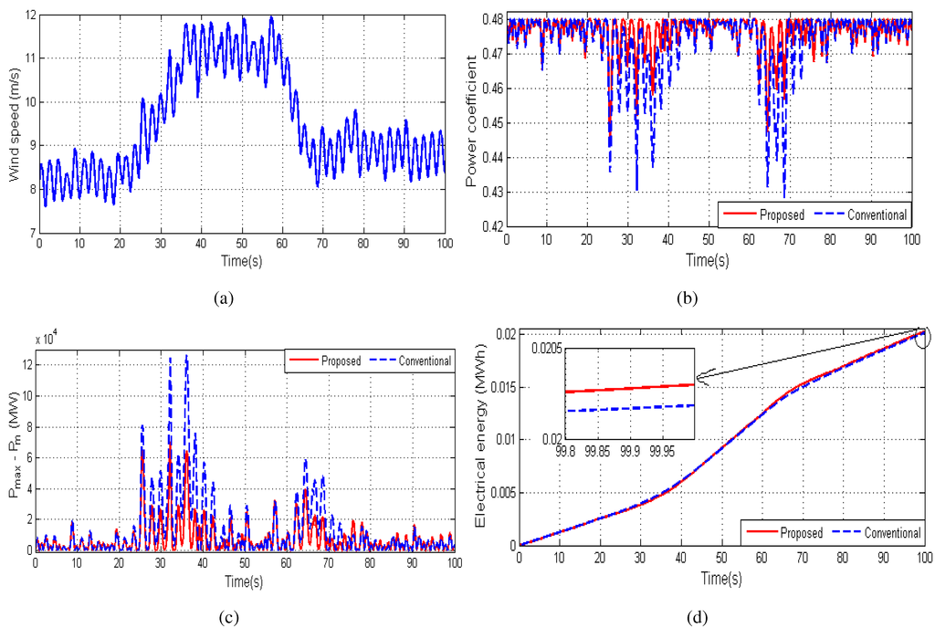
Figure 9. Simulation results with the rapid wind profile: (a) wind speed profile; (b) power coefficient; (c) error between $P_{\max }$ and $P_m$; (d) electrical energy output.

5. Conclusions

This paper proposes an MPPT method for DFIG wind turbines. The proposed MPPT method ensures that the wind turbine can track the maximum power operation point better than can a wind turbine with the conventional MPPT-curve method, as verified via the simulation of a 1.5-MW DFIG wind turbine. These simulation results indicate that $C_p$ reached $C_{p\max }$, λ was varied around ${\lambda }_{\mathrm{opt}}$ and the electrical energy output of the generator was higher than that achieved with the conventional method. Furthermore, with the designed controllers, the error between desired values and actual ones converged to zero. Thus, the proposed control method is proven to achieve stable operations.

References

- Leon, A.E.; Farias, M.F.; Battaiotto, P.E.; Solsona, J.A.; Valla, M.I. Control strategy of a DVR to improve stability in wind farms using squirrel-cage induction generators. IEEE Trans. Power Syst. 2011, 26, 1609–1617. [Google Scholar] [CrossRef]
- Barakati, S.M.; Kazerani, M.; Aplevich, J.D. Maximum power tracking control for a wind turbine system including a matrix converter. IEEE Trans. Energy Convers. 2009, 24, 705–713. [Google Scholar] [CrossRef]
- Qiu, Y.; Zhang, W.; Cao, M.; Feng, Y.; Infield, D. An electro-thermal analysis of a variable-speed doubly-fed induction generator in a wind turbine. Energies 2015, 8, 3386–3402. [Google Scholar] [CrossRef]
- Abdullah, M.; Yatim, A.H.M.; Tan, C.; Saidur, R. A review of maximum power point tracking algorithms for wind energy systems. Renew. Sustain. Energy Rev. 2012, 16, 3220–3227. [Google Scholar] [CrossRef]
- Ganjefar, S.; Ghassemi, A.; Ahmadi, M. Improving efficiency of two-type maximum power point tracking methods of tip-speed ratio and optimum torque in wind turbine system using a quantum neural network. Energy 2014, 67, 444–453. [Google Scholar] [CrossRef]
- Lei, Y.; Mullane, A.; Lightbody, G.; Yacamini, R. Modeling of the wind turbine with a doubly fed induction generator for grid integration studies. IEEE Trans. Energy Convrers. 2006, 21, 257–264. [Google Scholar] [CrossRef]
- Jeong, H.G.; Seung, R.H.; Lee, K.B. An improved maximum power point tracking method for wind power systems. Energies 2012, 5, 1339–1354. [Google Scholar] [CrossRef]
- Tapia, A.; Tapia, G.; Ostolaza, J.; Saenz, J. Modeling and control of a wind turbine driven doubly fed induction generator. IEEE Trans. Energy Convers. 2003, 18, 194–204. [Google Scholar] [CrossRef]
- Fernandez, L.; Garcia, C.; Jurado, F. Comparative study on the performance of control systems for doubly fed induction generator (DFIG) wind turbines operating with power regulation. Energy 2008, 33, 1438–1452. [Google Scholar] [CrossRef]
- Wagner, H.; Mathur, J. Introduction to Wind Energy Systems: Basics, Technology and Operation; Springer-Verlag: Berlin/Heidelberg, Germany, 2013; pp. 63–64. [Google Scholar]
- Kim, H.W.; Kim, S.S.; Ko, H.S. Modeling and control of PMSG-based variable-speed wind turbine. Electr. Power Syst. Res. 2010, 80, 46–52. [Google Scholar] [CrossRef]
- Yang, L.; Xu, Z.; Stergaard, J.; Dong, Z.Y.; Wong, K.P.; Ma, X. Oscillatory stability and eigenvalue sensitivity analysis of a DFIG wind turbine system. IEEE Trans. Energy Convers. 2011, 26, 328–339. [Google Scholar] [CrossRef]
- Mishra, Y.; Mishra, S.; Li, F.; Dong, Z.Y.; Bansal, R.C. Small signal stability analysis of a DFIG-based wind power system under different modes of operation. IEEE Trans. Energy Convers. 2009, 24, 972–982. [Google Scholar] [CrossRef]
- Hu, J.; Nian, H.; Hu, B.; He, Y.; Zhu, Z.Q. Direct active and reactive power regulation of DFIG using sliding-mode control approach. IEEE Trans. Energy Convers. 2010, 25, 1028–1039. [Google Scholar] [CrossRef]
- Barambones, O.; Cortajarena, J.A.; Alkorta, P.; Durana, J.M.G. A real-time sliding mode control for a wind energy system based on a doubly fed induction generator. Energies 2014, 7, 6412–6433. [Google Scholar] [CrossRef]
- Khemiri, N.; Khedher, A.; Mimouni, M.F. Wind energy conversion system using DFIG controlled by backstepping and sliding mode strategies. Int. J. Renew. Energy Res. 2012, 2, 421–430. [Google Scholar]
- Beltran, B.; Ahmed-Ali, T.; Benbouzid, M. High-order sliding-mode control of variable-speed wind turbines. IEEE Trans. Ind. Electron. 2009, 56, 3314–3321. [Google Scholar] [CrossRef]
- Soliman, M.; Malik, O.P.; Westwick, D.T. Multiple model predictive control for wind turbines with doubly fed induction generators. IEEE Trans. Sustain. Energy 2011, 2, 215–225. [Google Scholar] [CrossRef]
- Wu, B.; Lang, Y.; Zargari, N.; Kouro, S. Power Conversion and Control of Wind Energy System; Wiley: Hoboken, NJ, USA, 2011. [Google Scholar]
- Abad, G.; López, J.; Rodríguez, M.A.; Marroyo, L.; Iwanski, G. Doubly Fed Induction Machine: Modelling and Control for Wind Energy Generation; Hanzo, L., Ed.; John Wiley & Sons: Hoboken, NJ, USA, 2011. [Google Scholar]
- Kim, Y.; Chung, I.; Moon, S. Tuning of the PI controller parameters of a PMSG wind turbine to mmprove control performance under various wind speeds. Energies 2015, 8, 1406–1425. [Google Scholar] [CrossRef]
- Hughes, F. M.; Anaya-Lara, O.; Jenkins, N.; Strbac, G. A power system stabilizer for DFIG-based wind generation. IEEE Trans. Power Syst. 2006, 21, 763–772. [Google Scholar] [CrossRef]
- Singh, M.; Santoso, S. Dynamic models for wind turbines and wind power plants. Available online: http://www.nrel.gov/docs/fy12osti/52780.pdf (accessed on 22 May 2015).
© 2015 by the authors; licensee MDPI, Basel, Switzerland. This article is an open access article distributed under the terms and conditions of the Creative Commons Attribution license (http://creativecommons.org/licenses/by/4.0/).